www.atmos-meas-tech.net/10/617/2017/ doi:10.5194/amt-10-617-2017
© Author(s) 2017. CC Attribution 3.0 License.
Improved methodologies for continuous-flow analysis of
stable water isotopes in ice cores
Tyler R. Jones1, James W. C. White2, Eric J. Steig3, Bruce H. Vaughn1, Valerie Morris1, Vasileios Gkinis4, Bradley R. Markle3, and Spruce W. Schoenemann3
1Institute of Arctic and Alpine Research, University of Colorado, Boulder, CO 80309-0450, USA 2Institute of Arctic and Alpine Research and Department of Geological Sciences, University of Colorado,
Boulder, CO 80309-0450, USA
3Department of Earth and Space Sciences, University of Washington, Seattle, Washington 98195-1310, USA 4Centre for Ice and Climate, Niels Bohr Institute, University of Copenhagen, Copenhagen, Denmark
Correspondence to:Tyler R. Jones ([email protected]) Received: 6 April 2016 – Discussion started: 26 July 2016
Revised: 22 January 2017 – Accepted: 30 January 2017 – Published: 27 February 2017
Abstract. Water isotopes in ice cores are used as a climate proxy for local temperature and regional atmospheric circu-lation as well as evaporative conditions in moisture source regions. Traditional measurements of water isotopes have been achieved using magnetic sector isotope ratio mass spec-trometry (IRMS). However, a number of recent studies have shown that laser absorption spectrometry (LAS) performs as well or better than IRMS. The new LAS technology has been combined with continuous-flow analysis (CFA) to im-prove data density and sample throughput in numerous prior ice coring projects. Here, we present a comparable semi-automated LAS-CFA system for measuring high-resolution water isotopes of ice cores. We outline new methods for par-titioning both system precision and mixing length into liquid and vapor components – useful measures for defining and improving the overall performance of the system. Critically, these methods take into account the uncertainty of depth reg-istration that is not present in IRMS nor fully accounted for in other CFA studies. These analyses are achieved using sam-ples from a South Pole firn core, a Greenland ice core, and the West Antarctic Ice Sheet (WAIS) Divide ice core. The mea-surement system utilizes a 16-position carousel contained in a freezer to consecutively deliver ∼1 m×1.3 cm2ice sticks to a temperature-controlled melt head, where the ice is con-verted to a continuous liquid stream and eventually vaporized using a concentric nebulizer for isotopic analysis. An inte-grated delivery system for water isotope standards is used for calibration to the Vienna Standard Mean Ocean Water
(VSMOW) scale, and depth registration is achieved using a precise overhead laser distance device with an uncertainty of ±0.2 mm. As an added check on the system, we per-form inter-lab LAS comparisons using WAIS Divide ice sam-ples, a corroboratory step not taken in prior CFA studies. The overall results are important for substantiating data obtained from LAS-CFA systems, including optimizing liquid and va-por mixing lengths, determining melt rates for ice cores with different accumulation and thinning histories, and remov-ing system-wide mixremov-ing effects that are convolved with the natural diffusional signal that results primarily from water molecule diffusion in the firn column.
1 Introduction
Copen-hagen in 1952, then on the visible layers of icebergs in the North Atlantic, and later in the Camp Century ice core (de-scribed in Dansgaard, 2005). Since these early experiments, a large collection of ice core water isotope records have been recovered from the Greenland Ice Sheet, the Antarctic Ice Sheet, and many high-latitude and/or high-altitude ice caps. These records have been instrumental in understanding cli-mate change over annual to millennial timescales, includ-ing abrupt climate change events (Dansgaard et al., 1989; Grootes et al., 1993; Alley, 2000), the bipolar seesaw (WAIS Divide Project Members, 2015), and glacial–interglacial cy-cles (Petit et al., 1999).
Traditional measurements of water isotopes have been ac-complished using customized preparation systems and iso-tope ratio mass spectrometry (IRMS; see a full list of abbre-viations in Table 1). Typically, water samples are analyzed discretely using 3–5 cm intervals of ice. Isotopic ratios of oxygen are usually obtained using a CO2–H2O equilibration
method (Epstein et al., 1953; Craig et al., 1963). For hydro-gen isotopes, a variety of methods have been used, including H2–H2O equilibration using a platinum catalyst and
reduc-tion of water with uranium, zinc, or chromium (Bigelseisen et al., 1952; Bond, 1968; Coleman et al., 1982; Coplen et al., 1991; Vaughn et al., 1998; Huber and Leuenberger, 2003).
Advances in high-precision laser absorption spectroscopy (LAS) methods are now widely adopted as an alternative to IRMS methods (Kerstel et al., 1999; Lis et al., 2008; Gupta et al., 2009; Brand et al., 2009). There are currently two main LAS methods used: cavity ring-down laser spec-troscopy (CRDS; manufactured by Picarro, Inc.) and off-axis integrated cavity output laser spectroscopy (OA-ICOS; man-ufactured by Los Gatos Research). The CRDS method (uti-lized in this study) requires the input of water vapor into a detection cavity that confines and reflects laser pulses using a series of mirrors. By comparing the extinction of a laser pulse at different frequencies in an empty cavity and in a cavity filled with water vapor, water isotope concentrations can be determined (Crosson, 2008).
Systems have been developed that continuously deliver water vapor into LAS measurement devices. The technique, known as continuous-flow analysis (CFA), is accomplished by slowly melting a solid ice stick into a continuous liquid stream, which is then vaporized and injected into the LAS instrument. Gkinis et al. (2010, 2011) established the CFA framework for water isotope analysis using LAS. In particu-lar, Gkinis reproduced traditional IRMS water isotope mea-surements in Greenland ice using a Picarro L1102-i CRDS instrument. Gkinis found that the precision of hydrogen and oxygen isotope measurements was comparable to IRMS. Substantial increases in depth resolution and shorter analysis time were realized. Maselli et al. (2013) expanded on Gki-nis’ technique by testing multiple new-generation Picarro de-vices (L2120-i and L2130-i) and found similar results. Later, Emanuelsson et al. (2015) used OA-ICOS to continuously analyze water samples from an ice core, achieving reductions
in isotopic step-change response time and memory effects. Other water isotope CFA techniques (not considered in this paper) have utilized a platinum catalyst for continuous mass spectrometry measurements (Huber and Leuenberger, 2005) or a thermal conversion elemental analyzer (TC/EA) coupled to a mass spectrometer (Sharp et al., 2001). CFA has also widely been used for chemical measurements in ice cores (e.g., Röthlisberger, 2000; Osterberg et al., 2006; Bigler et al., 2011; and Rhodes et al., 2013).
1.1 Goals of this study
In this study, we present a semi-automated water isotope CRDS-CFA system developed at the Institute of Arctic and Alpine Research (INSTAAR) Stable Isotope Lab (SIL). We analyzeδD,δ18O, and deuterium excess values in a series of ice samples from Greenland and Antarctica. New methods are used to test the precision of the isotopic data. We present “full-system” precision tests using replicate ice samples to account for multiple sources of uncertainty on the CRDS-CFA system. We then present steps to create isotopically dis-tinct ice sticks to evaluate the impulse response of the system, which yields a CFA system mixing length. The mixing length is a measure of 1σ displacement of water molecules from their original position in the solid ice sample. This is impor-tant for two reasons: (1) the system mixing length needs to be distinguished from the effects of diffusion occurring nat-urally in the ice sheet, and (2) based on the mixing length, system flow rates and the total mixing volume can be ad-justed to prevent isotopic signal attenuation in ice cores from low-accumulation drill sites. Based on the system wide mix-ing length, we propose a way to separate isotopic mixmix-ing effects in the liquid and vapor phase. This test is important for CFA systems that have complicated liquid-phase com-ponents, such as those systems analyzing multiple chemical species that require extra lengths of tubing to transport liq-uid water. We then perform inter-lab and inter-system iso-topic testing of firn ice and solid ice to determine how the CRDS-CFA system performs with ice of different densities. The results of this study will be used in the analysis of the West Antarctic Ice Sheet (WAIS) Divide ice core (WDC), the South Pole ice core (SPICE), and other ice cores in the future.
2 Data processing methodologies and evaluation 2.1 Water isotope measurements
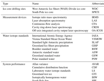
VS-Table 1.List of abbreviations used in this paper.
Type Name Abbreviation
Ice core drilling sites West Antarctic Ice Sheet (WAIS) Divide ice core WDC
South Pole ice core SPICE
Measurement devices Isotope ratio mass spectrometry IRMS
Laser absorption spectrometry LAS
Continuous-flow analysis CFA
Cavity ring-down laser spectroscopy CRDS Off-axis integrated cavity output laser spectroscopy OA-ICOS
Water isotope standards International Atomic Energy Agency IAEA Vienna Standard Mean Ocean Water VSMOW Standard light Antarctic precipitation SLAP Greenland Ice Sheet precipitation GISP
Boulder standard water BSW
Antarctic standard water ASW
Greenland standard water GSW
Polar standard water PSW
System performance Allan variance AVAR
Cumulative distribution function CDF Laboratory water isotope standards LS
Greenland test ice GTI
Isotopically homogenous water IHW
South Pole firn SPF
MOW has been set to 0 ‰ by the International Atomic En-ergy Agency (IAEA):
δsample=
R
sample
RVSMOW
−1
, (1)
whereRis the isotopic ratio18O/16O or D/H (i.e.,2H/1H) in the sample or VSMOW. The δ values (δ18O orδD) are thus deviations from VSMOW, usually expressed in parts per thousand (per mil or ‰). The deuterium excess parameter (dxs) is defined as function of both hydrogen and oxygen isotope ratios:
dxs=δD−8·δ18O. (2)
The dxs variable is not a direct isotopic measurement, but rather it is calculated from the direct measurement of oxy-gen and hydrooxy-gen isotope ratios. The precise calculation of dxs (‰) has historically been challenging because IRMS methodology requires that oxygen and hydrogen water iso-tope ratios be analyzed on separate systems using separate samples, which could increase uncertainty. The CRDS-CFA technique removes the potential for multi-system uncertainty because both isotopic values are measured simultaneously on a single sample with the same system.
2.2 Experimental system
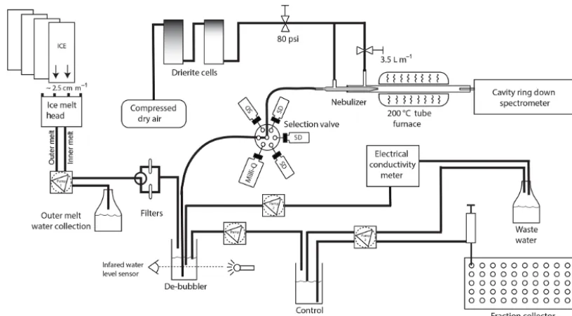
Figure 1.The INSTAAR CRDS-CFA system, showing sample flow from the ice melt head through the filter block and debubbler and onto the Valco stream selection valve, nebulizer, furnace, and Picarro L-2130-i CRDS instrument.
rate of 2.5 cm min−1. This melt rate can be increased or de-creased by changing the temperature of the melt head. To pre-vent ice sticks from wedging against the acrylic tube during ice melt, we affix small vibrating devices to the tubes, where vibrational frequency is controlled by a variable DC power supply. A laser distance device tracks the rate at which the ice stick melts and decreases in length, with an uncertainty of ±0.2 mm (Dimetix FLS-CH-10, Dimetix AG, Switzerland). The remote measurement of the laser allows for immediate change of ice over the melt head without reconfiguration of any mechanical measurement device.
For the liquid-to-gas conversion component of the system, liquid water is drawn away from the melt head interface us-ing peristaltic pumps (Masterflex L/S 7534-04). Liquid water from the outer square catchment of the melt head is collected for other purposes. The inner square catchment is pumped at a rate matching that of the ice stick melt. This liquid water is pushed through an 8 µm disposable filter backed by a 10 µm PEEK frit (IDEX A-411). The liquid water is pushed through filters to allow for ice with ash and dust layers to be analyzed without compromising the system.
The filtered water then enters a 2 mL open-top glass vial where bubbles can escape (debubbler). The flow rate into the debubbler is 3.1 m min−1. An overflow tube, kept at a height of 6 mm from the bottom of the vial, regulates the height of the water. The vial has an inner diameter of 9.96 mm. A por-tion of the debubbled water is used as primary flow (i.e., for isotopic measurements), which is aspirated from the debub-bler through a 0.062500 OD, 0.02000 ID tubing via a selec-tor valve (VICI Cheminert 10P-0392L). The primary flow rate is 0.1 m min−1. The primary water is then channeled
Figure 2.A typical CRDS-CFA analysis day consisting of the anal-ysis of 12 m of ice core sticks from the WDC. The light grey regions show the analysis of four calibrated laboratory isotopic standards. The dark grey regions show the analysis of mock ice. The promi-nent white region shows the analysis of ice core sticks separated by short sections of push ice every fourth ice stick.
split where mixing with dry air and flash vaporization takes place at a temperature of 170◦C (Gkinis et al., 2010, 2011). An advantage of the nebulizer is the wider ID, reducing the susceptibility to clogging from microparticles. The spray is directed into a 20.0×1.8 cm Pyrex vaporizing tube that is heated to 200◦C inside a ceramic tube furnace (Whatlow VC400N06A). Additional dry air (< 30 ppm H2O) is added at
a rate of∼3.5 L min−1to dilute the water vapor and achieve a final water vapor content of∼25 000 ppm H2O, which is
within the optimal range of 20 000–40 000 ppm H2O for the
Picarro L2130-i. Finally, the water vapor flows through an intake line (3.175 mm OD×2 mm ID×10 cm stainless-steel tubing) inserted approximately 5 cm into the Pyrex vaporiz-ing tube. This line is plumbed into a Picarro L2130-i analyzer by an open-split interface. Any excess vapor is vented away from the instrumentation.
At the Valco six-port stream selection valve, the primary water flow can be switched off, allowing another auxil-iary port to be switched on. Each auxilauxil-iary port is con-nected to 30 mL glass vials of laboratory isotopic water stan-dards, which can be analyzed and used for calibration of ice core measurements to international reporting standards. Ad-ditional water streams (secondary flow) are pumped from the debubbler to an electrical conductivity (EC) measure-ment cell (Amber Science 1056) and to a fraction collector (Gilson 215). The EC measurement allows for the compar-ison of chemical signatures at a known depth between labs. The fraction collector is used to archive water samples for discrete analysis and as a safeguard against system failures. It is programmed to partially fill approximately twenty-five 2 mL glass vials for every meter of ice melted, approximat-ing a discrete ice samplapproximat-ing resolution of about 4.0 cm. 2.3 A typical analysis day
On a given analysis day, we perform a sequence of measure-ments related to calibration and correction (Fig. 2). At the beginning and end of an analysis day, established laboratory isotopic water standards are analyzed to calibrate the ice core data. These laboratory isotopic water standards are annually calibrated to IAEA primary standards (VSMOW2, SLAP2, and GISP). We use four laboratory standards – Boulder stan-dard water (BSW), Antarctic stanstan-dard water (ASW), Green-land standard water (GSW), and Polar standard water (PSW) – that together provide a range of∼244 and∼31 ‰ forδD andδ18O, respectively. Each laboratory standard is analyzed twice for 20 min at the beginning and end of the day (four times total), except for PSW, which is analyzed only two times total. Table 2 contains a summary of isotopic standards. To characterize isotopic mixing throughout the sys-tem, three small (20 cm×13 mm2) sections of laboratory-prepared ice are made from batches of isotopically distinct waters withδD values of approximately−240 ‰ for the first and third sections and−120 ‰ for the second section (here-after referred to as mock ice). The mock ice is created by
filling lay-flat tubing with isotopically homogenous water (IHW), freezing the water at −60◦C in chilled ethanol to minimize fractionation, and cutting the ice into small sec-tions using a band saw. The mock ice is analyzed twice per day at the beginning and end of an ice core melt sequence. Each instance of mock ice analysis is used to determine how the CRDS-CFA system is responding to an instantaneous step change in isotopic values (in this case, a change from −240 to −120 ‰, and vice versa). This mixing effect can be quantified using transfer and impulse functions, which we discuss later in this paper.
An ice core melt sequence occurs in between analysis of laboratory isotopic water standards and mock ice. Key vari-ables are closely monitored during this time, including water concentration in the Picarro instrument, the melt rate, and depth registration. During the ice core melt sequence, every set of four ice cores is separated by 20 cm sections of iso-topically homogenous ice with aδD value of about−115 ‰ (hereafter referred to as push ice). The push ice isotopic value is much heavier than the surrounding ice core samples to en-sure that they can be easily distinguished from each other. The push ice also maintains a consistent thermal load on the melt head and consistent water vapor delivery to the Picarro during routine maintenance tasks that include changing the filters and cleaning the melt head.
2.4 Post-measurement data processing
A graphical user interface (GUI) developed in Python is used to automate procedures and collect auxiliary data related to carousel positioning, active Valco port, ice core depth regis-tration, quality control (e.g., water level in the debubbler and melt rate), electrical conductivity, and commenting. These auxiliary data are collected using serial ports via a Moxa UPort 1610-8, and all data are recorded at the same data fre-quency as the isotopic data generated by the Picarro L2130-i (L2130-in thL2130-is case, at approxL2130-imately∼1.18 Hz intervals; 0.85 s intervals). With the use of an algorithm supplied by Picarro Inc., the ancillary data are exported continuously to a raw text file along with data from the CRDS. The raw data are then post-processed offline by a separate semi-automated Python script.
Table 2.Water isotope standards in units of per mil (‰). The laboratory standards (BSW, ASW, GSW, and PSW) were calibrated to primary standards (VSMOW2, SLAP2, and GISP) in March 2010. The primary standards are reported with errors given by the IAEA. The laboratory standards are reported with a precision value given by the average standard deviation (1σ) of multiple isotopic determinations across multiple analysis platforms (IRMS and CRDS). In parentheses, the combined uncertainty of the laboratory standard and each primary standard is given, added in quadrature.
Standards δD δD uncertainty δ18O δ18O uncertainty
VSMOW2 0 0.3 0 0.02
SLAP2 −427.5 0.3 −55.5 0.02
GISP −189.5 1.2 −24.76 0.09
BSW −111.8 0.2 (1.3) −14.19 0.02 (0.10) ASW −239.3 0.3 (1.3) −30.35 0.04 (0.10) GSW −298.7 0.2 (1.3) −38.09 0.03 (0.10) PSW −355.6 0.2 (1.3) −45.43 0.05 (0.11)
2.4.1 Isotope calibration
Raw values from the CRDS system require calibration to known values of isotopic laboratory standards (as described in Sect. 2.3). Since isotopic mixing effects in the CRDS-CFA impede instrument response to the large and abrupt changes in laboratory standards, we use the average of the last 5 min of a 20 min total analysis to minimize the mixing effect (dis-cussed further in Sect. 2.4.3). The “measured” (i.e., raw) values are plotted versus their “known” (i.e., assigned) VS-MOW2 calibrated values. From the plot of measured (yaxis) vs. known (xaxis) values, a linear regression is used to define a calibration slope (mcalibrated)and y intercept (bcalibrated).
We then correct the GSW isotopic standard using the fol-lowing equation:
xcorrected=
ymeasured−bcalibrated
mcalibrated
, (3)
where ymeasured is the averaged GSW value (as described
above) measured on the CRDS-CFA system andxcorrectedis
the GSW value calibrated to the VSMOW2-SLAP2 scale. This same calibration is done for all ice core isotopic mea-surements.
2.4.2 System performance
In addition to calibration, we also use the laboratory isotopic standards to define measures of precision and bias for the CRDS-CFA system downstream of the Valco stream selec-tion valve. These values can be tracked through time as a per-formance indicator of the system. Precision is defined as the degree of internal agreement among independent measure-ments made under specific conditions, while bias is defined as the difference of the test results and an accepted reference value. In this case, the precision (downstream of the selector valve) is determined by taking the average standard deviation of each of the last 5 min of each 20 min laboratory standard run, while the bias (downstream of the selector valve) is de-fined as the difference of the measured GSW value from its
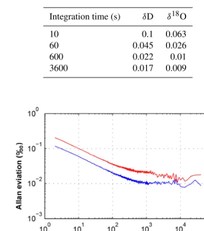
Table 3.Selected Allan deviation values (‰) for a 7 h analysis of isotopically homogenous water on the CRDS-CFA system.
Integration time (s) δD δ18O
10 0.1 0.063
60 0.045 0.026
600 0.022 0.01
3600 0.017 0.009
Figure 3.A 7 h analysis of Allan deviation forδD (red) andδ18O (blue) on the CRDS-CFA using isotopically homogenous water va-por.
known value. Over a period of 216 measurement days, the average precision and average bias forδD were 0.25±0.04 and 0.40±0.12 ‰ (1σ ), respectively. For δ18O, the aver-age precision and averaver-age bias values were 0.03±0.02 and −0.01±0.02 ‰ (1σ ), respectively. In Sect. 3, we define a precision value that takes into account all components of the CRDS-CFA system downstream of the melt head.
a parcel of vapor is present in the laser cavity). The Allan variance is defined as
AVAR2(τ )= 1 2(n−1)
n−1 X
i=1
(y(τ )i+1−y(τ )i)2, (4)
where τ is the integration time, y(τ ) is the average value of the measurements in an integration bin of length τ,nis the total number of bins, and AVAR is the Allan variance. The idea of integration bins simply refers to taking a long sequence of data and dividing it into smaller successive bins of a certain averaging timeτ, and then averaging the values in each bin to determine values fory(τ ).
We determine Allan deviation (the square root of Allan variance) for a continuous flow of isotopically homogenous water into the CRDS-CFA on a daily basis. The Allan de-viation values for an 11 h run are plotted in Fig. 3, and se-lected Allan deviation values are shown in Table 3. At small τ (∼3 s), Allan deviation is highest due to instrument mea-surement noise. At longerτ (∼3 to 1000 s), Allan deviation decreases because the sample is analyzed longer, and the in-strument measurement noise will average out. At ∼1000 s, a noise floor is reached, and longerτ does not improve the measurement results. At even longerτ, Allan deviation will again increase due to instrument drift from long-term tem-perature changes, componentry degradation, or other fac-tors. This increase is not observed in the data, as shown in Fig. 3. The Allan deviation plot we provide extends to 40 000 s (11 h), and from Fig. 1 a typical analysis day lasts about 50 000 s (∼14 h). Since we measure standards twice per day (morning and evening), the maximum temporal dis-tance between standard measurements and any ice core data point is about 7 h. The Allan deviation plot shows instrument stability up to 11 h, thus demonstrating that isotopic calibra-tions occur at sufficiently short timescales to account for any possible long-term drift in the system. The Allan deviation results shown here are similar to those shown in Fig. 4 of Gkinis et al. (2010) for a comparable CRDS-CFA system.
Relative to a set flow rate, an increase in integration time decreases the resolution of measured ice core data. There-fore, a choice must be made between the integration time and the amount of smoothing introduced into an ice core record. The Allan deviation tests described above inform these deci-sions relative to sample input originating at the Valco stream selection valve. In Sect. 3.1, we show that it is important to also use replicate ice sticks to analyze system performance for sample input originating at the melt head.
2.4.3 Mixing length calculations
Isotopic mixing effects occur in the CRDS-CFA system. Pos-sible contributors to the mixing effect include liquid mix-ing in tubmix-ing and the debubbler, liquid drag on tubmix-ing walls, vapor mixing downstream of the nebulizer, vapor interac-tions with two Picarro instrument filters (Mykrolis
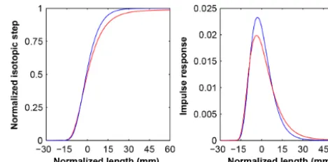
Wafer-Figure 4. The log–log CDF transfer functions (left) and skew-normal impulse response functions (right) of the CRDS-CFA sys-tem forδD (red) andδ18O (blue). The normalized functions are fit-ted to a mock ice isotopic step change inδD of approximately−240 to−120 ‰. The normalized length scale is calculated using an av-erage melt rate of 2.5 cm min−1. Note that the impulse response ofδD is slightly wider than forδ18O, which could possibly arise from diffusional effects in the system, differing interactions of wa-ter molecules with the Picarro filwa-ters, and differing memory effects within the Picarro cavity.
gard) prior to entering the laser cavity, adsorption of water molecules onto the laser cavity walls, and diffusional effects that can occur at any point in the CRDS-CFA system. To characterize the mixing, a transfer function and impulse re-sponse function of the system can be defined using mock ice or laboratory water standards. The transfer function is the system response to an instantaneous isotopic step change at the melt head or Valco stream selection valve. The im-pulse response function is the first derivative of the trans-fer function. The standard deviation of the impulse response corresponds to the mixing length (often referred to as diffu-sion length in other publications), which defines the average movement of a water molecule in the time or depth domain relative to its original position in the ice sample or within a vial of water. Figure 4 shows transfer functions and im-pulse response functions of the CRDS-CFA system forδD andδ18O.
In previous work by Gkinis et al. (2010, 2011), a trans-fer function is fit to an isotopic step change using a scaled version of the cumulative distribution function (CDF) of a normal distribution described by
δmodel(t )=
C10
2
1+erf
t−t
o
σn √
2
+C20, (5)
whereC10 andC20 are isotopic step-change values,t is the
time,to is the initial time, and σn is the standard deviation (i.e., the mixing length) – all of which are determined by least-squares optimization. The impulse response of the sys-tem is described by a Gaussian:
Gn(t )= 1 σn
√ 2πe
−t2
We modified this approach because the system response to an isotopic step change is skewed (see Fig. 4). We instead fit a transfer function in the form of a lognormal CDF multiplied with a lognormal CDF (log–log fit):
δmodel(t )=
1 2
1+erf
t−µ 1
σ1 √
2
·1 2
1+erf
t−µ2
σ2 √
2
, (7)
whereµ1,µ2,σ1, andσ2are determined by least-squares
op-timization. The impulse response function is found by fitting a skew-normal probability density function (PDF; Azzalini and Valle, 1996) to the first derivative of the log–log transfer function:
δmodel(t )=2φ (t )8(αt ), (8)
where φ (t ) is the standard normal PDF,8(t ) is the stan-dard normal CDF, andαis a shape parameter. The transform t→ t−ε
ω introduces the location parameter ε and the scale parameterω. The mixing length termσsis then recovered by
β=√ α
1+α2, (9)
σs2=ω2
1−2β 2
π
, (10)
whereα,ε, andωare estimated by least-squares optimiza-tion.
Since mixing effects in the system may stem from poten-tially different processes occurring in liquid and vapor phases of the CRDS-CFA system, we attempted to separate the por-tion of the system where vapor dominates. We evaluated mix-ing effects for the whole system (liquid+vapor) by evaluat-ing mixevaluat-ing lengths determined from step changes in mock ice (σmock ice). This includes mixing in the melt head, tubing,
de-bubbler, nebulizer, Pyrex furnace tube, and laser cavity. Sim-ilarly, mixing lengths were determined from step changes in liquid laboratory isotopic standards (σLS)introduced at the
Valco valve. The process downstream of this valve is domi-nated by the vapor phase, with a short 10 cm section of tubing where liquid water is transported from the Valco to the neb-ulizer.
Using Eqs. (5)–(10), mixing length values were deter-mined forσmock iceandσLS(Table 4), where the difference in
quadrature between the two is the amount of mixing occur-ring in the liquid phase (σLQD)of the CRDS-CFA system. We
find that the majority of the mixing in the CRDS-CFA sys-tem occurs in the liquid phase (i.e., downstream of the melt head to the Valco stream selection valve), while the remain-der occurs in the vapor phase of the system (i.e., downstream of the Valco stream selection valve to the laser cavity).
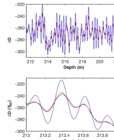
Figure 5.A comparison of the WAIS Divide ice core δD signal measured on the CRDS-CFA system (black); the CRDS-CFA mix-ing corrected isotopic signal usmix-ingσmock ice of 0.8 cm (red); and a correction for a typical West Antarctic diffusion value of 6.5 cm (blue), which represents diffusional processes occurring naturally in the ice sheet (see Fig. 6 of Cuffey and Steig, 1998). The mix-ing introduced by the CRDS-CFA is only a fraction of the diffusion occurring naturally in the ice sheet.
Theσmock ice values are not valid for firn ice, which has
much lower densities than deeper ice due to the bubbles and vapor pathways that are present in the firn. The remainder of this paper, except for Sect. 3.3, relates to tests of solid ice beneath the firn column. To illustrate the importance of σmock ice, consider a series of solid ice core samples that have
an average layer thickness of∼23.0 cm yr−1(a typical value at∼200 m depth in the WAIS Divide ice core). Aσmock ice
value of∼1 cm would have almost no effect on the attenua-tion of the natural signal. However, if the average layer thick-ness were ∼2.0 cm yr−1 (a typical value for very low ac-cumulation sites in East Antarctica), thenσmock ice= ∼1 cm
would have a larger attenuation affect on the isotopic sig-nal. For low-accumulation sites, it may be necessary to ad-just the melt rate or decrease the total mixing volume of a CRDS-CFA system so as to decrease the σmock ice values.
Figure 5 shows a comparison of isotopic signal corrections usingσmock icefor the CRDS-CFA system vs. a typical
dif-fusion length occurring naturally from difdif-fusional processes in the Antarctic Ice Sheet at the location of the WAIS Divide ice core. In the data output file, values ofσmock ice and melt
Table 4. Mean mixing length values from 50 determinations of mock ice step changes (σmock ice) and for laboratory isotopic standards step changes (σLS). The difference in quadrature ofσmock iceandσLSis the amount of mixing occurring in the liquid phase of the CRDS-CFA system (σLQD). Mixing length values for both skew and normal impulse response functions are given in seconds and in meters (in parentheses), based on a melt rate of 2.5 cm min−1. Values with an asterisk represent 1σvariability in meters.
σLS σmock ice σLQD
Fit type δD δ18O δD δ18O δD δ18O
Skew 10.3 9.6 18.7 17.7 15.6 14.9
(0.004) (0.004) (0.008) (0.007) (0.007) (0.006) (*0.0002) (*0.0002) (*0.0009) (*0.0009)
Normal 10.2 9.4 19.1 17.4 16.1 14.6
(0.004) (0.004) (0.008) (0.007) (0.007) (0.006) (*0.0002) (*0.0002) (*0.0008) (*0.0009)
Table 5.The average bias and the standard deviation of the mean (‰) for 50 determinations of isotopic step-change corrections us-ing mock ice (i.e.,δD step-change values of approximately−240 to −120 ‰). Each data bin includes 20 consecutive data points (span-ning∼17 s of analysis time), increasing fromcn=0.5. The data in each bin are averaged for each determination. Corrected values of dxs are calculated from the correctedδD andδ18O values. From cn=0.5, about 100 s is needed to achieve greater than 98 % of the expected mock ice value of−120 ‰. For comparison, the calcula-tion of the standard deviacalcula-tion of the mean for 50 determinacalcula-tions of 17 s averages of isotopically homogenous water yields values for δD,δxO, and dxs of 0.01, 0.01, and 0.05 ‰, respectively. The iso-topically homogenous water was allowed to run through the CRDS-CFA system for 1 h before the 17 s averages were determined.
Bin δD δ18O dxs
0–17 s −0.36 (0.28) 0.14 (0.05) −1.49 (0.38) 17–34 s −0.06 (0.30) 0.06 (0.03) −0.55 (0.15) 34–51 s −0.15 (0.27) 0.01 (0.04) −0.21 (0.07) 51–68 s −0.17 (0.18) −0.01 (0.03) −0.10 (0.06) 68–85 s −0.18 (0.13) −0.01 (0.02) −0.09 (0.05) 85–102 s −0.16 (0.10) −0.01 (0.02) −0.05 (0.04)
2.4.4 Isotopic step-change correction
During a typical analysis day, every fourth ice core stick is separated by isotopically distinct push ice. Ideally, the iso-topic shift between push ice and the beginning of an ice core stick at the melt head would register instantaneously on the CRDS instrument. However, a substantial mixing effect is evident in the first∼5–7 cm of an ice core sample. This ef-fect can be partially corrected for by separately determining mixing coefficients (cn), quantified using an instantaneous shift in mock ice isotopic values at the melt head. The iso-topic values of the mock ice sticks are approximately−240 and −120 ‰. As the water for the mock ice sticks moves through the CRDS-CFA system, the water will mix together, resulting in a smoothed transition over time (rather than an
Figure 6.Mixing corrections for mock ice (left) and the beginning of an ice core section (right). The ice core mixing correction is based upon a known step-function change defined by the mock ice, from which mixing coefficients are determined. Red represents raw un-corrected isotopic data with no memory correction, black represents VSMOW corrected data with the memory correction applied, blue dots represent 3 cm IRMS discrete samples, and the grey region rep-resents the depth range of corrected data that would otherwise be discarded. Note that the time variable represents the amount of run time on a given day.
instantaneous transition) as measured by the CRDS instru-ment. For example, at a time of 5 s after a shift in mock ice at the melt head (not including the delay in transport from the melt head to the CRDS instrument), the measured isotopic value may only be 2 % of the expected value. After 40 s the measured value may be 40 % of the expected value, and after 100 s, the measured value may be 95 % of the expected value. For these three examples, thecncoefficients would be 0.02, 0.40, and 0.95, respectively. To remove noise from the cn calculation, we average mock ice isotopic values, normalize between 0 and 1, and apply a cubic spline. The water isotope step-change correction is described by Eq. (4) of Vaughn et al. (1998):
δmc=
δm−δmp(1−cn)
cn
whereδmis the measured isotopic value at indexn,δmpis the
previously measured isotopic value atn−1,cnis the memory coefficient atn, andδmcis the corrected isotopic value atn.
An example of an isotopic step-change correction, applied to an isotopic shift between push ice and the beginning of an ice core stick, is shown in Fig. 6. For cn≥0.65, the correction saves an additional∼2.25–3.15 cm of data that would oth-erwise be discarded. For a typical deep ice core of 3000 m, there are 750 step changes (every fourth ice core stick). This correction saves∼16.9–23.7 m of isotopic data. In the data output file we produce, the depths of isotopic step-change corrections are flagged so researchers can decide whether to include some or all of these data in their calculations. In Ta-ble 5, we provide standard error estimates for isotopic step-change corrections of mock ice sticks for different bins of data atcn≥0.5.
3 Ice core measurement results 3.1 Greenland test ice
To test CRDS-CFA precision for the entire system, nine sticks of solid ice were cut from a single meter of Green-land test ice (GTI) at about 400 m depth. The ice sticks were obtained from the National Science Foundation Na-tional Ice Core Laboratory (Lakewood, Colorado) and were a by-product of the initial tests of the US Deep Ice Sheet Coring Drill performed in Greenland in 2006 (Johnson et al., 2007). The same drill was deployed in West Antarctica to ob-tain the WAIS Divide ice core, which we discuss in Sect. 3.2. Seven of the nine GTI sticks were analyzed on the CRDS-CFA system, three of which were broken into parts to test depth registration methodology. As stated previously, these ice sticks are melted at a rate of 2.5 cm min−1, and data are recorded on the CRDS instrument at 0.85 s intervals. The fi-nal two GTI sticks were discretely sampled at 1 and 5 cm increments, melted into vials, and analyzed on a separate Pi-carro L2130-i.
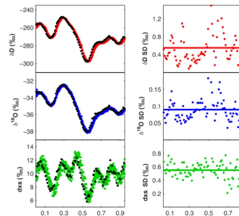
The isotopic data for the seven 1 m long GTI sticks an-alyzed on the CRDS-CFA system were measured at sub-millimeter resolution. These data were then averaged to 1 cm successive values (GTI-1 cm) for each stick, resulting in seven values at each 1 cm increment, from which a standard deviation was determined. This resulted in a total of 100 standard deviation values, and the mean of these values is used to estimate the full-system precision (Fig. 7). We find full-system precision values (1σ ) forδD,δ18O, and dxs of 0.55, 0.09, and 0.55 ‰, respectively. For comparison, tradi-tional IRMS measurements using uranium reduction forδD and CO2–H2O equilibration forδ18O are commonly reported
with a precision of about 1.0 and 0.1 ‰, respectively. The resulting dxs precision using these two measurement tech-niques is about 1.3 ‰.
Figure 7.Greenland test ice (GTI) for a nominal 1 m section. In the left column, seven GTI sticks measured on the CRDS-CFA system averaged to 1 cm increments forδD (red dots),δ18O (blue dots), and dxs (green dots) compared with discrete 1 cm samples (black dots) measured on a Picarro L2130-I using the average of three injec-tions. In the right column, the standard deviation of seven GTI val-ues is taken at each 1 cm increment (red, blue, and green dots). The average standard deviation is shown by the horizontal line, which represents the full-system precision (1σ) forδD,δ18O, and dxs.
Figure 8. Scatterplots of GTI comparisons of CRDS-CFA vs. discrete data. Seven GTI sticks were analyzed on the CRDS-CFA system, down-sampled to 1 cm, and averaged. The discrete data were sampled at 1 cm and analyzed on a separate Picarro L-2130i using the average of three injections. The black line is the best-fit linear regression. The 1σ errors for the slope and intercept of the δD regression are 0.0035 and 0.9346, respectively. For the δ18O regression, the errors are 0.0045 and 0.1555, respectively. For the dxs regression, the errors are 0.0315 and 0.3116, respectively.
significantly larger than the noise added on the vapor side of the system.
As a final analysis using GTI, the reproducibility of GTI-1 cm CRDS-CFA data and GTI-1 cm discrete CRDS data is com-pared. We define reproducibility as the closeness of the agreement between results of measurements of the same measure and carried out under changed conditions of mea-surement. In this case, the same water samples are analyzed using a Picarro L2130-i, but the exact conditions of measure-ment are different, in that some samples are analyzed on the CFA-CRDS system, while others are analyzed by discrete sample injection into a CRDS instrument. A scatterplot and linear regression of the resulting data for the two measure-ment types give a slope,y intercept, andR2 value (Fig. 8). The coefficient of determination values (R2)forδD andδ18O are 0.9981 and 0.9970, respectively, while dxs remains inher-ently more difficult to measure with anR2value of 0.8763. Because this test shows the comparison of seven GTI sticks
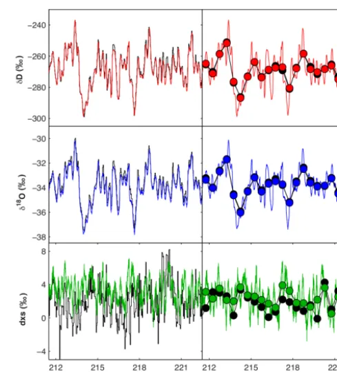
Figure 9.Data from the WDC over a depth range of∼212–222 m. In the left column, high-resolution CRDS-CFA data forδD (red line), δ18O (blue line), and dxs (green line) are compared with traditional high-resolution IRMS discrete samples (black lines). In the right column, comparison of high-resolution CRDS-CFA data (red, blue, and green lines), low-resolution University of Washing-ton CRDS discrete samples (black dots), and down-sampled CRDS-CFA data (red, blue, and green dots).
analyzed on CRDS-CFA compared with a single ice stick measured discretely on CRDS, theR2 values represent the reproducibility of the average of seven ice sticks vs. a sin-gle ice stick carried out under changed conditions of mea-surement. We explore the reproducibility of sets of single ice sticks for IRMS and CRDS in the following section. 3.2 WAIS Divide ice core tests
The reproducibility of traditional IRMS discrete measure-ments and CRDS-CFA measuremeasure-ments (both analyzed at the INSTAAR SIL) was tested on the WAIS WDC over depths of ∼212–222 m (Fig. 9). The discrete samples (3 cm cuts) were measured using a uranium reduction technique forδD (Vaughn et al., 1998) and a CO2–H2O equilibration method
Table 6.The isotopic measurement precision (1σ) of varying parts of the CRDS-CFA system (‰). The difference in quadrature of the full-system precision derived from GTI (system) and the precision derived from IHW (vapor-side) gives an estimate of the noise added on the preparation side of the system (prep-side). The prep-side val-ues include noise added to the isotopic signal upstream of the Valco valve, while the vapor-side values include noise added to the iso-topic signal downstream of the Valco valve.
Measurement System Vapor-side Prep-side
δD 0.55 0.09 0.54
δ18O 0.09 0.04 0.08
dxs 0.55 0.32 0.45
δD andδ18O values while retaining the same signal ampli-tude. Furthermore, if the calibrations forδD andδ18O were offset in different intervals of ice, this could possibly cause the IRMS dxs values to be negative. Indeed, the dxs values in the IRMS samples are decreased and more negative over the 10 m section as compared to CRDS-CFA, sometimes with offsets of up to 7 ‰. Another possible explanation for neg-ative IRMS dxs values is that there was fractionation within some of the discrete sample vials over time.
A second WDC reproducibility test was performed be-tween high-resolution CRDS-CFA measurements and resolution discrete CRDS measurements (Fig. 9). The low-resolution data were measured at the University of Wash-ington (UW) using a Picarro 2120i at ∼50 cm increments (Steig et al., 2013). To determine inter-lab reproducibility, we averaged the high-resolution CRDS-CFA data to the exact low-resolution discrete CRDS increments; we refer to this as “down-sampling”. Over a depth of∼212–222 m, scatterplot comparisons of the down-sampled high-resolution data and low-resolution measurements haveR2values forδD,δ18O, and dxs of 0.9871, 0.9944, and 0.2885, respectively. The slopes are 1.0113, 0.9928, and 0.7658, respectively, and the 1σ errors for the slopes are 0.0175, 0.0065, and 0.1960, re-spectively. Theyintercepts are 3.2457,−0.1730, and 0.4152, respectively, and the 1σerrors for theyintercepts are 4.6688, 0.2235, and 0.6750, respectively.
The combination of WDC test results leads to the follow-ing conclusions: (1) the δD andδ18O data are reproducible between traditional IRMS and CRDS-CFA techniques (both measured at INSTAAR), albeit with an occasional offset in magnitude but not amplitude. We suggest, but cannot prove, that the offset is due to standard water calibration difficulties using IRMS, or due to outdated sample storage techniques that introduced additional fractionation in the IRMS samples. (2) The dxs data between IRMS and CRDS-CFA (both mea-sured at INSTAAR) are not reproduced well, possibly due to the uncertainty introduced by multi-system IRMS measure-ments or because the discrete samples underwent additional fractionation due to storage procedures. (3) However, the CRDS-CFA analysis of GTI (measured at INSTAAR) shows
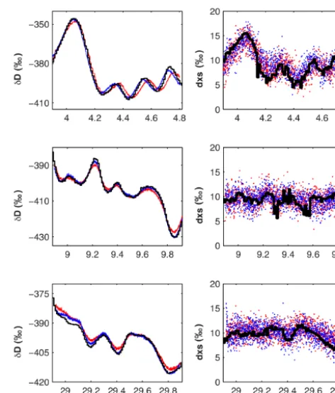
Figure 10.Replicate SPF ice measurements ofδD and dxs at depths of∼4, 9, and 29 m, corresponding to densities of 340, 386, and 562 kg m−3, respectively. The red and blue data are from SPF sticks analyzed on the CRDS-CFA system, and the black data are 1 cm discrete samples analyzed on a separate Picarro L2130-i.
that the full-system precision of dxs has a low average stan-dard deviation of 0.55 ‰ and, when compared with discrete CRDS samples, has a highR2value of 0.88. This shows that the INSTAAR CRDS-CFA is capable of reliably measuring dxs at high frequencies (annual to multi-year). (4) Yet inter-lab reproducibility (INSTAAR CRDS-CFA vs. UW CRDS) of down-sampled dxs has a lowR2 value of 0.29, but still within the same range of values between∼1 and 4 ‰. These results suggest that the inherent noise in dxs measurements may make this parameter most useful at timescales of cen-turies to millennia when the range of WDC dxs increases to ∼0 to 12 ‰ (Markle et al., 2017).
3.3 South Pole firn tests
rate to increase or decrease unexpectedly. Furthermore, we have not devised a reliable way to test σmock ice for firn, as
the interconnected vapor pathways and trapped air bubbles are difficult to replicate in the lab. For this reason, we can only test the reliability of CRDS-CFA firn measurements by comparing the CFA measurements to discrete samples over the same intervals of ice. To test the repeatability of CRDS-CFA firn measurements, two identical 1 m sections from 4, 9, and 29 m depth in a South Pole firn core are analyzed under the same conditions of measurement (hereafter referred to as South Pole firn: SPF). These CRDS-CFA firn measurements are then compared with a third identical 1 m SPF section dis-cretely sampled at 1 cm increments using a Picarro L2130-i (Fig. 10).
Based upon a steady-state Herron and Langway density model (Herron and Langway, 1980), the SPF sticks have es-timated densities of 340, 386, and 562 kg m−3at depths of
4, 9, and 29 m, respectively (assuming an average accumu-lation rate of 0.085 m yr−1, average temperature of−50◦C, average snow density in the top 2 m of 300 kg m−3, and pore close-off density of 804.3 kg m−3). For comparison, the den-sity of snow at the surface of the WAIS Divide ice core is ∼370 kg m−3. Because of the low-density SPF sticks, the melt rate was increased from 2.5 to 4.4 cm min−1to prevent wicking during this experiment. We observed that no wick-ing occurred durwick-ing the meltwick-ing process.
The data show that a loss in δD amplitude not surpass-ing 11% occurred in the CRDS-CFA data relative to the discretely sampled data, while maximum depth registration offsets were 4, < 0.5, and < 0.5 cm at 4, 9, and 29 m depth, respectively. At 4 m depth, the phase of the CRDS-CFA and discreteδD signal is offset by about 3 cm over the last ∼60 cm of the SPF section, which is likely related to im-precise depth registration on the CRDS-CFA due to the in-creased melt rate, fluctuations in the melt rate, or unobserved wicking. At 29 m depth, CRDS-CFAδD measurements are anomalously higher than discrete measurements in the first 20 cm. The dxs values for the CRDS-CFA and 1 cm discrete signals have the same pattern and range of values, except for small offsets in the last∼60 cm of the 4 m depth section and again at∼9.30 and∼9.55 m. We note that the ability to an-alyze the SPF samples was likely improved due to long stor-age times that allowed the ice sticks to sinter, increasing the structural integrity of the samples. We have found in other subsequent experiments that short storage times cause low-density firn sticks to collapse when placed vertically in the CFA system, introducing large uncertainty in depth registra-tion and essentially unusable isotopic data.
3.4 Method comparison
The CRDS-CFA setup presented in this paper (INSTAAR; CRDS L-2130i) can be compared with similar studies from Victoria University of Wellington (VUW; OA-ICOS “custom 2014 setup”) and the University of Copenhagen (UC; CRDS
L-2140i; Emanuelsson et al., 2015), as well as the Desert Re-search Institute (DRI; CRDS L-2120i and L-2130i; Maselli et al., 2012). Allan deviation values ofδD at 103s for IN-STAAR, VUW, UC, DRI-2120i, and DRI-2130i are 0.020, 0.060, 0.048,∼0.15, and∼0.20 ‰, respectively. Forδ18O, these values are 0.010, 0.030, 0.011,∼0.06, and∼0.02 ‰, respectively. Allan deviation values of δD at 104s for IN-STAAR, VUW, and UC are 0.013,∼0.04, and ∼0.11 ‰, respectively. Forδ18O, these values are 0.008, ∼0.06, and ∼0.006 ‰, respectively. No Allan deviation values at 104s are given for DRI. Mixing length values of ice introduced at the melt head for INSTAAR (δD isotopic step change of 120 ‰) and both DRI instruments (step-change amount not clearly given) are 19.1 and ∼24 s, respectively. For the equivalentδ18O step change, these values are 17.4 and ∼24 s. Note that the DRI study did not differentiate between δD and δ18O for mixing lengths. Mixing length values of ice introduced at the selector valve for INSTAAR (δD iso-topic step change of 120 ‰), VUW (step change of 124 ‰), UC (step change of 253 ‰), and both DRI instruments (step-change amount not clearly given) are 10.2, 18.5, 93.6, and 17 s, respectively. For the equivalentδ18O step change, these values are 9.4, 18.4, 90.3, and 17 s, respectively. Specific se-lector valve placements and total mixing volume can be ref-erenced in each manuscript’s system schematic.
The important difference between this study and prior studies is that we perform tests of replicate ice sticks origi-nating at the melt head, rather than testing Allan deviation of sample input originating at the selector valve. This is an im-portant distinction, as there are factors that affect the isotopic data prior to the selector valve, such as depth registration and mixing in the debubbler.
4 Conclusions
We have presented a high-resolution CFA system based on CRDS technology that is specifically designed for water iso-tope analysis of ice cores. The CFA system converts∼1 m ice sticks into a continuous liquid water stream, which is then vaporized and analyzed on a CRDS instrument. The full sys-tem builds from previous water isotope CFA studies (Gkinis et al., 2010, 2011; Maselli et al., 2013; Emanuelsson et al., 2015) and includes novel improvements to the ice delivery mechanism and the melt head. In terms of Allan deviation and response time, the CRDS-CFA system presented here performed similarly to previously published systems from the US, New Zealand, and Denmark (Gkinis et al., 2010, 2011; Maselli et al., 2013; Emanuelsson et al., 2015).
sug-gest that researchers instead utilize high-resolution discrete samples for firn column measurements. For solid ice, we used seven identical Greenland ice core sticks to quantify the precision of the CRDS-CFA system. This technique is pre-viously unpublished and helps quantify as many sources of uncertainty on the CRDS-CFA system as possible, including depth registration and sample mixing. Additionally, we mea-sured West Antarctic ice core sticks to test the reproducibility of two sets of measurements: (1) traditional magnetic sector IRMS vs. CRDS-CFA system measurements, and (2) inter-lab comparisons of CFA and discrete measurements on the same type of CRDS instrument. We find that the CRDS-CFA system provides a ∼6-fold time savings and an order-of-magnitude improvement in data density compared to tradi-tional IRMS methods. Inter-lab comparisons ofδD andδ18O were strongly correlated (R2values of 0.9871 and 0.9944, respectively).
One exception to these solid ice results is found in the dxs measurements. At the highest frequencies (multi-year to decadal), we found discrepancies in comparisons of both inter-lab CRDS measurements of dxs and in CRDS and IRMS measurements of dxs. Contrary to this, however, are the dxs results measured solely on the CRDS-CFA system presented in this paper. We found that dxs can be replicated at high frequencies, demonstrated by tests of identical Green-land ice core sticks. Furthermore, despite slightly different impulse response functions for δD andδ18O, the dxs mea-sured from replicate ice sticks on the CRDS-CFA system is strongly correlated (R2=0.88) with discrete CRDS dxs values measured on the same replicate ice. This indicates a negligible artifact in dxs calculations arising from the differ-ing impulse response functions. To better understand high-resolution measurements of dxs, we suggest additional multi-lab studies be undertaken.
The overall results are in line with prior ice core CFA studies. Gkinis et al. (2011) cite combined measurement un-certainty values of 0.2, 0.06, and 0.5 ‰ for δD,δ18O, and dxs, respectively. Maselli et al. (2013) and Emanuelsson et al. (2015) report similar results. However, unlike these prior studies, the precision values cited in this paper (0.55, 0.09, and 0.55 ‰, respectively) were determined using seven repli-cate ice core sticks and therefore cannot be compared di-rectly. We suggest that future CFA studies include determi-nations of precision using replicate ice sticks, as this is most representative of the variations introduced into water isotope measurements downstream of the ice core melt head. In ad-dition, Allan deviation comparisons should be made, but this only takes into consideration the sample flow downstream of the selector valve, rather than downstream of the melt head. Similarly, total mixing length values can be measured down-stream of the melt head and downdown-stream of the selector valve, yielding insights into system behavior. We find the majority of mixing occurs between the melt head and selector valve.
5 Data availability
The high-resolution WDC Water Isotope Data can be found at http://gcmd.gsfc.nasa.gov/search/Metadata.do?entry= NSF-ANT10-43167.
The low-resolution WDC Water Isotope Data can be found at http://gcmd.gsfc.nasa.gov/search/Metadata.do? entry=WAIS_Divide_Isotope_Data.
Additional data inquiries can be made to the corresponding author, Tyler R. Jones ([email protected]).
Competing interests. The authors declare that they have no conflict of interest.
Acknowledgements. This work was supported by US National Science Foundation (NSF) grants 0537930, 0537593, 1043092, and 1043167. The authors would like to thank all field crew, laboratory staff, students, and principal investigators involved with the project. Field and logistical activities were managed by the WAIS Divide Science Coordination Office at the Desert Research Institute, Reno, NE, USA, and the University of New Hampshire, USA (NSF grants 0230396, 0440817, 0944266, and 0944348). The National Science Foundation Division of Polar Programs funded the Ice Drilling Program Office (IDPO), the Ice Drilling Design and Operations (IDDO) group, the National Ice Core Laboratory (NICL), the Antarctic Support Contractor, and the 109th New York Air National Guard. Finally, we would like to thank the Centre for Ice and Climate at the Niels Bohr Institute, University of Copenhagen, for support in the design of the analysis system used in this study.
Edited by: R. Koppmann
Reviewed by: J. Rudolph and one anonymous referee
References
Allan, D. W.: Statistics of atomic frequency standards, P. IEEE, 54, 221–230, 1966.
Alley, R. B.: Ice-core evidence of abrupt climate changes, P. Natl. Acad. Sci. USA, 97, 1331–1334, 2000.
Azzalini, A. and Dalla Valle, A.: The multivariate skew-normal dis-tribution, Biometrika, 83, 715–726, 1996.
Bigeleisen, J., Perlman, M. L., and Prosser, H. C.: Conversion of hydrogenic materials to hydrogen for isotopic analysis, Anal. Chem., 24, 1356–1357, 1952.
Bigler, M., Svensson, A., Kettner, E., Vallelonga, P., Nielsen, M. E., and Steffensen, J. P.: Optimization of high-resolution continuous flow analysis for transient climate signals in ice cores, Environ. Sci. Technol., 45, 4483–4489, 2011.
Bond, G. C.: Catalysis by metals, Annu. Rep. Prog. Chem. A, 65, 121–128, 1968.
pure water samples and alcohol/water mixtures, Rapid Commun. Mass Sp., 23, 1879–1884, 2009.
Coleman, M. L., Shepherd, T. J., Durham, J. J., Rouse, J. E., and Moore, G. R.: Reduction of water with zinc for hydrogen isotope analysis, Anal. Chem., 54, 993–995, 1982.
Coplen, T. B., Wildman, J. D., and Chen, J.: Improvements in the gaseous hydrogen-water equilibration technique for hydrogen isotope-ratio analysis, Anal. Chem., 63, 910–912, 1991. Craig, H., Gordon, L. I., and Horibe, Y.: Isotopic exchange effects
in the evaporation of water: 1. Low-temperature experimental re-sults, J. Geophys. Res., 68, 5079–5087, 1963.
Crosson, E. R.: A cavity ring-down analyzer for measuring atmo-spheric levels of methane, carbon dioxide, and water vapor, Appl. Phys. B, 92, 403–408, 2008.
Cuffey, K. M. and Steig, E. J.: Isotopic diffusion in polar firn: impli-cations for interpretation of seasonal climate parameters in ice-core records, with emphasis on central Greenland, J. Glaciol., 44, 273–284, 1998.
Dansgaard, W.: Stable isotopes in precipitation, Tellus, 16, 436– 468, 1964.
Dansgaard, W., White, J. W. C., and Johnsen, S. J.: The abrupt ter-mination of the Younger Dryas climate event, Nature, 339, 532– 534, 1989.
Dansgaard, W.: Frozen Annals – Greenland Icecap Research, Niels Bohr Institute, Narayana Press, Odder, Denmark, available at: www.narayanapress.dk (last access: 1 April 2016), ISBN: 87-990078-0-0, 124 pp., 2005.
Emanuelsson, B. D., Baisden, W. T., Bertler, N. A. N., Keller, E. D., and Gkinis, V.: High-resolution continuous-flow analysis setup for water isotopic measurement from ice cores using laser spec-troscopy, Atmos. Meas. Tech., 8, 2869–2883, doi:10.5194/amt-8-2869-2015, 2015.
Epstein, S., Buchsbaum, R., Lowenstam, H. A., and Urey, H. C.: Revised carbonate-water isotopic temperature scale, Geol. Soc. Am. Bull., 64, 1315–1326, 1953.
Gkinis, V., Popp, T. J., Johnsen, S. J., and Blunier, T.: A contin-uous stream flash evaporator for the calibration of an IR cavity ring-down spectrometer for the isotopic analysis of water, Isot. Environ. Healt. S., 46, 463–475, 2010.
Gkinis, V., Popp, T. J., Blunier, T., Bigler, M., Schüpbach, S., Ket-tner, E., and Johnsen, S. J.: Water isotopic ratios from a contin-uously melted ice core sample, Atmos. Meas. Tech., 4, 2531– 2542, doi:10.5194/amt-4-2531-2011, 2011.
Grootes, P. M., Stuiver, M., White, J. W. C., Johnsen, S., and Jouzel, J.: Comparison of oxygen isotope records from the GISP2 and GRIP Greenland ice cores, Nature, 366, 552–554, 1993. Gupta, P., Noone, D., Galewsky, J., Sweeney, C., and Vaughn, B. H.:
Demonstration of high-precision continuous measurements of water vapor isotopologues in laboratory and remote field deploy-ments using wavelength-scanned cavity ring-down spectroscopy (WS-CRDS) technology, Rapid Commun. Mass Sp., 23, 2534– 2542, 2009.
Herron, M. M. and Langway Jr, C. C.: Firn densification: an empir-ical model, J. Glaciol., 25, 373–385, 1980.
Huber, C. and Leuenberger, M.: Fast high-precision on-line de-termination of hydrogen isotope ratios of water or ice by continuous-flow isotope ratio mass spectrometry, Rapid Com-mun. Mass Sp., 17, 1319–1325, 2003.
Huber, C. and Leuenberger, M.: On-line systems for continuous wa-ter and gas isotope ratio measurements, Isot. Environ. Healt. S., 41, 189–205, 2005.
Johnsen, S. J., Dahl-Jensen, D., Gundestrup, N., Steffensen, J. P., Clausen, H. B., Miller, H., Masson-Delmotte, V., Sveinbjörns-dottir, A. E., and White, J.: Oxygen isotope and palaeotemper-ature records from six Greenland ice-core stations: Camp Cen-tury, Dye-3, GRIP, GISP2, Renland and NorthGRIP, J. Quater-nary Sci., 16, 299–307, 2001.
Johnson, J. A., Mason, W. P., Shturmakov, A. J., Haman, S. T., Sendelbach, P. J., Mortensen, N. B., Augustin, L. J., and Dah-nert, K. R.: A new 122 mm electromechanical drill for deep ice-sheet coring (DISC): 5. Experience during Greenland field test-ing, Ann. Glaciol., 47, 54–60, 2007.
Jouzel, J. and Merlivat, L.: Deuterium and oxygen 18 in precipita-tion: modeling of the isotopic effects during snow formation, J. Geophys. Res.-Atmos., 89, 11749–11757, 1984.
Jouzel, J., Alley, R. B., Cuffey, K. M., Dansgaard, W., Grootes, P., Hoffmann, G., Johnsen, S. J., Koster, R. D., Peel, D., Shuman, A., Stievenard, M., Stuiver, M., and White, J.: Validity of the temperature reconstruction from water isotopes in ice cores, J. Geophys. Res.-Oceans, 102, 26471–26487, 1997.
Kavanaugh, J. L. and Cuffey, K. M.: Space and time variation of δ18O andδD in Antarctic precipitation revisited, Global Bio-geochem. Cy., 17, 1017, doi:10.1029/2002GB001910, 2003. Kerstel, E. T., Van Trigt, R., Reuss, J., and Meijer, H. A. J.:
Simulta-neous determination of the2H/1H,17O/616O, and18O/16O isotope abundance ratios in water by means of laser spectrome-try, Anal. Chem., 71, 5297–5303, 1999.
Lis, G., Wassenaar, L. I., and Hendry, M. J.: High-precision laser spectroscopy D/H and 18O/16O measurements of microliter natural water samples, Anal. Chem., 80, 287–293, 2008. Markle, B. R., Steig, E. J., Buizert, C., Schoenemann, S. W., Bitz,
C. M., Fudge, T. J., Pedro, J. B., Ding, Q., Jones, T. R., White, J. W., and Sowers, T.: Global atmospheric teleconnections during Dansgaard-Oeschger events, Nat. Geosci., 10, 36–40, 2017. Maselli, O. J., Fritzsche, D., Layman, L., McConnell, J. R., and
Meyer, H.: Comparison of water isotope-ratio determinations us-ing two cavity rus-ing-down instruments and classical mass spec-trometry in continuous ice-core analysis, Isot. Environ. Healt. S., 49, 387–398, 2013.
Mook, W.: Environmental Isotopes in the Hydrological Cycle, IHP-V Technical Documents in Hydrology no. 39, UNESCO/IAEA, Paris/Vienna, 2000.
Osterberg, E. C., Handley, M. J., Sneed, S. B., Mayewski, P. A., and Kreutz, K. J.: Continuous ice core melter system with dis-crete sampling for major ion, trace element, and stable isotope analyses, Environ. Sci. Technol., 40, 3355–3361, 2006. Petit, J. R., Jouzel, J., Raynaud, D., Barkov, N. I., Barnola, J. M.,
Basile, I., Bender, M., Chappellaz, J., Davis, M., Delaygue, G., and Delmotte, M.: Climate and atmospheric history of the past 420 000 years from the Vostok ice core, Antarctica, Nature, 399, 429–436, 1999.
Röthlisberger, R., Bigler, M., Hutterli, M., Sommer, S., Stauffer, B., Junghans, H. G., and Wagenbach, D.: Technique for continuous high-resolution analysis of trace substances in firn and ice cores, Environ. Sci. Technol., 34, 338–342, 2000.
Sharp, Z. D., Atudorei, V., and Durakiewicz, T.: A rapid method for determination of hydrogen and oxygen isotope ratios from water and hydrous minerals, Chem. Geol., 178, 197–210, 2001. Steig, E. J., Ding, Q., White, J. W. C., Kuttel, M., Rupper, S. B.,
Neumann, T. A., Neff, P. D., Gallant, A. J. E., Mayewski, P. A., Taylor, K. C., Hoffmann, G., Dixon, D. A., Schoenemann, S. W., Markle, B. R., Fudge, T. J., Schneider, D. P., Schauer, A. J., Teel, R. P., Vaughn, B. H., Burgener, L., Williams, J., and Ko-rotkikh, E.: Recent climate and ice-sheet changes in West Antarc-tica compared with the past 2000 years, Nat. Geosci., 6, 372–375, 2013.
Vaughn, B. H., White, J. W. C., Delmotte, M., Trolier, M., Cattani, O., and Stievenard, M.: An automated system for hydrogen iso-tope analysis of water, Chem. Geol., 152, 309–319, 1998. WAIS Divide Project Members: Precise interpolar phasing of abrupt
climate change during the last ice age, Nature, 520, 661–665, 2015.