www.atmos-meas-tech.net/9/1637/2016/ doi:10.5194/amt-9-1637-2016
© Author(s) 2016. CC Attribution 3.0 License.
An automatic precipitation-phase distinction algorithm for optical
disdrometer data over the global ocean
Jörg Burdanowitz1, Christian Klepp2, and Stephan Bakan1
1Max Planck Institute for Meteorology, Bundesstraße 53, Hamburg, Germany 2University of Hamburg, CliSAP/CEN, Bundesstraße 55, Hamburg, Germany Correspondence to: Jörg Burdanowitz ([email protected])
Received: 27 November 2015 – Published in Atmos. Meas. Tech. Discuss.: 21 December 2015 Revised: 10 March 2016 – Accepted: 28 March 2016 – Published: 13 April 2016
Abstract. The lack of high-quality in situ surface precipita-tion data over the global ocean so far limits the capability to validate satellite precipitation retrievals. The first systematic ship-based surface precipitation data set OceanRAIN (Ocean Rainfall And Ice-phase precipitation measurement Network) aims at providing a comprehensive statistical basis of in situ precipitation reference data from optical disdrometers at 1 min resolution deployed on various research vessels (RVs). Deriving the precipitation rate for rain and snow requires a priori knowledge of the precipitation phase (PP). Therefore, we present an automatic PP distinction algorithm using avail-able data based on more than 4 years of atmospheric mea-surements onboard RV Polarstern that covers all climatic regions of the Atlantic Ocean. A time-consuming manual PP distinction within the OceanRAIN post-processing serves as reference, mainly based on 3-hourly present weather in-formation from a human observer. For automation, we find that the combination of air temperature, relative humidity, and 99th percentile of the particle diameter predicts best the PP with respect to the manually determined PP. Excluding mixed phase, this variable combination reaches an accuracy of 91 % when compared to the manually determined PP for 149 635 min of precipitation from RV Polarstern. Including mixed phase (165 632 min), an accuracy of 81.2 % is reached for two independent PP distributions with a slight snow over-prediction bias of 0.93. Using two independent PP distribu-tions represents a new method that outperforms the conven-tional method of using only one PP distribution to statisti-cally derive the PP. The new statistical automatic PP distinc-tion method considerably speeds up the data post-processing within OceanRAIN while introducing an objective PP prob-ability for each PP at 1 min resolution.
1 Introduction
Rare and often low-quality gauge-based surface reference data sets challenge the in situ validation of oceanic precip-itation as observed by passive and active microwave satellite sensors (Taylor, 2000; Adler et al., 2012). Over land, radar and gauge-based precipitation monitoring networks cover a large fraction of the land surface for more than 2 decades, which qualifies them to validate precipitation satellite esti-mates (Schneider et al., 2014). However, the ocean surface lacks dense long-term in situ precipitation monitoring net-works. Furthermore, existing coastal and island-based pre-cipitation measurements may not fully represent oceanic precipitation because the measured particle size distribu-tions (PSDs), precipitation rates, and accumuladistribu-tions may dif-fer from those measured over the open ocean (Kidd and Lev-izzani, 2011). However, Bumke and Seltmann (2012) found no difference between PSDs over coastal areas and ocean. Most existing in situ oceanic precipitation data sets sam-ple measurements from low-quality rain gauges on volun-tary observing ships (VOSs; Kent et al., 2010) or buoy ar-rays (Weller et al., 2008). Many of these in situ ocean data sets include present weather observations but lack quantita-tive estimates of precipitation. The high-latitude ocean com-pletely lacks precipitation measurements that sample solid and mixed-phase precipitation. However, recent and future precipitation satellite estimates demand high-quality in situ quantitative precipitation estimates including snowfall over the global ocean.
rain gauges with horizontal catchment surfaces face a large undercatch (Yuter and Parker, 2001; Michelson, 2004). In the extratropics, mixed-phase and solid precipitation cause fur-ther difficulties strongly adding to the undercatch (Goodison, 1978) of horizontally oriented measuring surfaces. In con-trast, optical instruments with a vertically oriented measur-ing surface such as disdrometers perform better at capturmeasur-ing precipitation under high wind speeds, though varying wind directions are challenging. Optical disdrometers are thus de-noted as the reference in situ instrument to measure precipi-tation (Taylor, 2000).
To provide systematic high-quality in situ precipitation data over the ocean, the long-term Ocean Rainfall And Ice-phase precipitation measurement Network (OceanRAIN; Klepp, 2015) applies automatic optical disdrometers of type ODM470 that are deployed onboard sea-going research ves-sels (RVs) for operation in all climatic regions. The ODM470 was developed to measure under high wind speed and fre-quently varying wind directions. Its cylindrical measuring volume ensures being independent from the wind-driven in-cidence angle of the falling hydrometeors while a wind vane keeps the measuring volume perpendicular to the instanta-neous wind direction. The ODM470 accuracy lies within a range of 3 % rain accumulation limited to rainfall at various wind conditions with respect to an improved ship rain gauge including side collectors on RV Alkor on the Baltic Sea (Bumke and Seltmann, 2012). Compared to an ANS410 WMO-reference rain gauge over land (Lanza and Vuerich, 2009), the ODM470 deviates by 2 % under low wind speed (Klepp, 2015). For snow, a predecessor of the current ODM470 agreed with the observer’s log during the Lofoten Cyclones campaign (LOFZY; Klepp et al., 2010) in detecting snowfall events. More recent results for measuring snow and mixed-phase precipitation are expected soon from the WMO Solid Precipitation InterComparison Experiment (SPICE) at Marshall field site in Boulder (CO, USA), where the ODM470 was compared against a multitude of in situ solid precipitation instruments for more than 2 years. The ODM470 suits well to measure various types of precipitation under open-ocean conditions onboard sea-going RVs.
The deployment of the ODM470 on several RVs allows to sample OceanRAIN precipitation data from all climate zones including the cold-season high latitudes. This requires a precipitation-phase (PP) distinction between rain, snow, and mixed phase in order to provide correct precipitation rates for disdrometer-measured PSDs. The PP information usually originates from human observers’ reports saved in the WMO present weather code ww (WMO, 2015). Efforts to automatize present weather observations impose high re-quirements on instruments such as present weather sensors. Automated present weather sensors encounter problems at temperatures around 0◦C as well as for light precipitation and small particle sizes (Merenti-Välimäki et al., 2001). High wind speed also complicates the PP determination because the wind speed strongly interferes with the particle fall speed
that solely carries the PP information. Thus, most studies to distinguish PPs limit the wind conditions to low wind speed or calm conditions (Löffler-Mang and Joss, 2000; Yuter et al., 2006; Ishizaka et al., 2013). Only few studies apply more so-phisticated instruments that use articulating particle size ve-locity (PARSIVEL) disdrometers to account for wind effects and thus directly derive the PP from the particle fall speed (Friedrich et al., 2013). More simply constructed instruments such as the ODM470 require ancillary data to determine the PP.
In OceanRAIN, we aim to replace the so far manual PP distinction method by an automatic algorithm for three main reasons. First, the manual method consumes a con-siderable amount of time and workforce because the 1 min precipitation data requires visual inspection of air tempera-ture, present weather observations, and theoretical rain and snow rate. Second, the human-based PP decision based on visual data inspection lacks objectivity while the decision itself remains non-transparent to the user. Third, temporal gaps exist between the 3-hourly present weather observa-tional timesteps, especially during nighttime adding to the uncertainty. Currently, no measures of this PP uncertainty are provided in the manual method. For these reasons, we present a new automatic PP distinction algorithm including a PP probability for OceanRAIN precipitation data that is also applicable to all other instruments sampling PSDs of precip-itation.
The new PP distinction algorithm follows a statistical ap-proach guided by many other studies that relate atmospheric predictors to the PP (Koistinen and Saltikoff, 1998; Fuchs et al., 2001; Dai, 2008; Froidurot et al., 2014). Most pre-vious work focuses on PP distinction over land only, while we introduce a new PP distinction algorithm over the ocean. Dai (2008) compares ocean and land areas using a relatively coarse time step of few to several hours depending on avail-ability of observations. In contrast, OceanRAIN offers at-mospheric measurements at 1 min resolution while present weather observations are limited to 3-hourly timesteps dur-ing daytime only. These high-resolution ancillary data from the RV combined with PSD data from the optical disdrometer enable a more accurate and reliable PP distinction.
2 Data and methods
Since 2010, OceanRAIN collects atmospheric data includ-ing precipitation rates on several RVs. Current permanent deployments include the German ships RV Polarstern (since June 2010), RV Meteor (since March 2014), RV Sonne (since November 2014), and the Russian ship Akademik Ioffe (since September 2010). The backbone of OceanRAIN is the op-tical disdrometer ODM470, which is explained in detail in Sect. 2.1. Section 2.2 introduces the manual method that has been used so far to retrieve the PP in OceanRAIN. These manually determined PPs function as a benchmark-ing reference for the new automatic PP distinction algorithm. For the algorithm development, we exclusively use RV Po-larstern data (Sect. 2.3) that contains a high fraction of high-latitude solid and mixed-phase precipitation being a prereq-uisite to develop a robust PP distinction algorithm. While Klepp (2015) describes the OceanRAIN data post-processing and quality checking before PP distinction we focus on pre-senting a new automatic PP estimation method that provides uncertainty information.
2.1 The ODM470
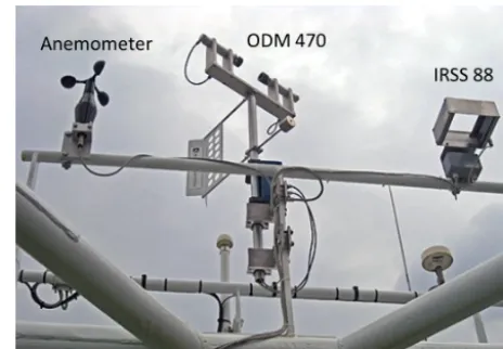
The ODM470 is an optical disdrometer to measure pre-cipitation, manufactured by the German company Eigen-brodt GmbH & Co KG near Hamburg (Germany). The in-strument consists of an infrared (IR) light-emitting diode (LED) at 880 nm and a photo diode receiver (Lempio et al., 2007). The IR-LED of the ODM470 is only activated once at least 8 particles per minute pass the active sensing area of the precipitation detector IRSS88 (Fig. 1, right) in order to increase IR-LED lifetime and exclude measurement arti-facts caused by birds or other non-precipitation objects. The IRSS88 switches off the ODM470 after 1 min without any particle passing the IRSS88 active sensing area. The entire ODM470 system was developed in a way to minimize unde-sired influences by changing wind directions and high wind speed. The ODM470 sensitive optical volume has a cylin-drical shape of 120 mm length and 22 mm in diameter. The cylindrical shape guarantees an independence from the inci-dence angle of the falling hydrometeors, which becomes cru-cial under high wind speeds and superstructure-induced local turbulence. Mounted on a pivotable axis, a wind vane ensures the optical volume to adjust perpendicular to the instanta-neous local wind direction. The ODM470 mounting height typically ranges between 30 and 45 m height, depending on the RV’s specifications (Fig. 1). This elevated deployment re-duces influences on the measured precipitation by splashing wave water.
During precipitation events, the falling hydrometeors at-tenuate the emitted IR radiation, which decreases the voltage signal measured. The duration of the voltage drop determines the particle transit time, that is, the total time it takes a par-ticle to pass through the optical volume of the disdrometer.
Figure 1. The image displays the automatic ODM470 measure-ment system including a cup anemometer, the optical disdrometer ODM470, and the precipitation detector IRSS88, deployed in the highest main mast at about 43 m height onboard RV Polarstern.
From the amplitude of the detector voltage drop the cross-sectional area can be deduced, which determines the particle diameter. The measured particle diameters are split into 128 logarithmically distributed size bins, of which the smallest is less than 0.02 mm and the largest corresponds to the op-tical volume diameter of 22 mm. However, wind- or wave-induced ship vibrations passed on to the instrument might cause artificial signals that are not distinguishable from real precipitation, which is why particles below bin 14 (0.43 mm diameter) are not considered in OceanRAIN. This exclusion of small particles also removes sea spray particles from the PSD spectra. The remaining particles are accumulated and binned over 1 min. From the resulting PSD, the precipitation rate PR (mm h−1) or liquid water equivalent (kg m−2h−1) after Großklaus (1996) can be calculated using
PR=3600· 128 X
bin=1
n(bin)·v(bin)·m(bin), (1)
wherev(bin) (m s−1) denotes the particle terminal fall speed andm(bin) (kg) the particle mass; both are parameterized.
n(bin) (m−3) denotes the PSD density per bin class that is calculated following Clemens (2002) by considering the ge-ometrical features, diameterd(m) and lengthl(m), the sam-pling timet (s) of the ODM470 as well as the sum of local wind speedUrel(m s−1) relative to the ship movement mea-sured by a cup anemometer, and the empirical terminal fall speedv(bin) (m s−1) as
n(bin)= N(bin)
l·d·t· q
Urel2 +
v(bin)2
. (2)
on the type of precipitation. Henceforth, we refer to precip-itation phase (PP), which means either liquid precipprecip-itation (rain), solid precipitation (e.g., snow or graupel), or mixed-phase precipitation. For rain the drop massml(kg), or liquid water content, and the particle terminal fall speedvl(m s−1) are well known and calculated using Eqs. (3) and (4) from Atlas and Ulbrich (1974), respectively.
ml=1000· 4
3π·(0.5D)
3 (3)
vl=9.65−10.3·e−600D (4) For snow, the measured cross-sectional area differs from the required maximum dimension of the particle due to the non-spherical shape of snowflakes. This difference requires ap-plying a transfer function. However, Lempio et al. (2007) found that the product of particle terminal fall speed and par-ticle mass (liquid water equivalent) as a function of cross-sectional area is in the same order of magnitude for var-ious frozen precipitation particle types. Hence, no transfer function between cross-sectional area and maximum diame-ter is required when using a spherical lump graupel assump-tion. The lump graupel assumption works well for frozen precipitation particles between 0.4 and 9 mm in diameter, whereas particles exceeding 9 mm in diameter rarely occur. Nevertheless, events with large particles introduce larger er-rors to the estimate in the same way as the retrieval qual-ity may largely differ for individual snowfall events. Over-all, no unique snowfall retrieval can be derived using optical disdrometers without recording the individual particle shape. Compared to a Geonor gauge, the optical disdrometer agreed well in most cases and overestimated a few light snowfall cases during the 1999/2000 winter period at Uppsala (Lem-pio et al., 2007). Following the lump graupel approximation by Hogan (1994), particle massms (Eq. 5) and particle ter-minal fall speedvs(Eq. 6) are calculated empirically as
ms=1.07·10−5·(100D)3.1, (5)
vs=7.33·(100D)0.78. (6) Klepp et al. (2010) observed lump graupel being the most frequently occurring precipitation type over the cold-season Norwegian Sea during the LOFZY campaign. Battaglia et al. (2010) discuss several sources of error for a snow-measuring PARSIVEL whereof those for particle shape and orienta-tion, margin effects, and coinciding particles also apply to the ODM470. However, the PARSIVEL is more sensitive to influences by wind speed and wind direction on the falling precipitation particles because the PARSIVEL has a fixed non-pivotable horizontal optical sensing area.
For mixed-phase precipitation, we generally use the snow retrieval (Eqs. 5 and 6) to calculate the precipitation rate within OceanRAIN because the absolute error of treating rain drops like snow particles, and thus underestimating the precipitation rate, results in a smaller error than vice versa.
In more than 90 % of the precipitating cases from RV Po-larstern in OceanRAIN the precipitation rate calculated with Eqs. (3) and (4) (theoretical rain rate) exceeds precipitation rate calculated with Eqs. (5) and (6) (theoretical snow rate) by a factor of 50 to 200. Accordingly, this large difference might cause large biases in the precipitation rate for mis-classified PP. Correctly mis-classified mixed-phase precipitation events might still strongly underestimate the precipitation rate if the instantaneous rain fraction sharply exceeds 0.5. The minute-aggregated fraction of liquid and solid particles cannot be identified by the ODM470 and would require an-cillary data such as a video disdrometer. More details on the instrumentation can be found in Lempio et al. (2007) while algorithm features are explained in Klepp (2015).
2.2 The manual PP distinction
re-Table 1. Translation of WMO present weather codes ww (WMO, 2015) into the three PPs from Petty (1995), Froidurot et al. (2014), and OceanRAIN. ww codes printed in bold can be translated into multiple PPs in OceanRAIN depending on ancillary data. “Indet./hail” denotes indeterminate precipitation or hail used for classification in Petty (1995).
Source Rain Snow Mixed phase Indet./hail
Petty (1995) 21, 25, 50–55, 58–65, 80–82, 91–92
22, 26, 70–78, 85-86
23–24, 56–57, 66–69, 79, 83– 84
20, 27–29, 87– 90, 93–99
OceanRAIN 20, 21, 25, 29,
50–67, 80–82, 91–92, 95, 97
20, 22, 26–27, 29, 70–79, 85– 86, 87–90, 93– 95, 96, 97, 99
23–24, 26–27, 29, 68–69, 83– 84, 87–90, 93– 95, 97
–
Froidurot et al. (2014) 58–65, 80–82, 91–92
70–79, 85–86 68–69, 83–84 –
quires visual inspection of PSDs and ancillary data collected onboard the RV.
The ww code from shipboard observations on RV Po-larstern is available 3 hourly during daytime only. Night-time conditions and PP changes between two consecutive 3-hourly observational time steps require ancillary data from the RV to derive the PP. By ancillary data we refer to atmo-spheric variables measured onboard the ship including the ODM470, such as air temperature, humidity, and precipita-tion rate. These ancillary data are available at a much higher resolution of 1 min compared to the 3-hourly observations. Initially, we assign the PP derived from the ww code directly to every single minute of precipitation that follows a 3-hourly observation as a first-guess information. If available, air tem-perature as one of the ancillary data serves to possibly cor-rect this first-guess PP. For near-freezing air temperatures, the manual procedure calculates the precipitation rate after Eq. (1) for rain (Eqs. 3 and 4) and snow (Eqs. 5 and 6) as-sumption separately. Large differences between theoretical rain and snow rate can help to identify a plausible PP. How-ever, if both theoretical rain and snow rate differ by much less than 2 orders of magnitude, their influence on the PP decision becomes negligible, which makes the PP more arbitrary. Ac-cordingly, the manual method might be biased by the worker who decides for a PP and the observer on the RV. For these reasons, we aim at developing an automatic PP distinction algorithm at 1 min resolution that statistically derives a PP from atmospheric measurements.
2.3 OceanRAIN data from RV Polarstern
The manual PP estimation has been applied to more than 4 years of OceanRAIN data from RV Polarstern (11 June 2010–8 October 2014). This period consists of several expe-ditions to Arctic and Antarctic regions. In addition to the high latitudes, RV Polarstern collected precipitation data from the tropics and subtropics when crossing the equator in the At-lantic Ocean six times (Fig. 2). The whole measuring pe-riod amounts to more than 268 000 min of precipitation
ex-Figure 2. Map illustrates ship tracks from RV Polarstern ALL data (11 June 2010–8 October 2014), whereby dots denote minutes of occurring precipitation classified by the manual PP distinction (cyan: rain; orange: mixed phase; purple: snow). Harbor times and minutes without precipitation are not shown. Left side denotes the fraction of each PP averaged per latitude.
warm-Table 2. OceanRAIN data sets from RV Polarstern divided into sub-data sets that are used in the analysis. While RSM (rain, snow, mixed phase) and ALL (all data) include the mixed phase, RS (rain, snow) sub-data exclude mixed-phase precipitation. RSM and RS include only those minutes with at least 20 particles of precipita-tion falling at mid- or high latitudes at air temperatures around the freezing point (see Sect. 2.3). The no-rain fraction (rain fraction subtracted from 1) yields the fraction frozen precipitation meaning snow cases for RS and snow and mixed phase for RSM and ALL.
Name Description Size (min) No rain (frac)
ALL Complete data sample 268 340 0.57
RSM Data sub-sample 165 632 0.61
(incl. mixed phase)
RS Data sub-sample 149 635 0.57
(excl. mixed phase)
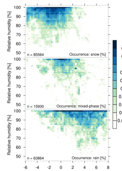
season RV Polarstern cruised on the southern hemispheric Atlantic Ocean and at the Antarctic. As an exception, RV Polarstern spent the whole year 2013 including austral cold season in the Southern Hemisphere, which explains the mul-titude of mixed-phase and snow precipitation cases between 45 and 75◦S that are not sampled at corresponding north-ern hemispheric latitudes. For the sake of polar research, RV Polarstern spends most research time in the polar regions, which results in a high time fraction of snow or mixed-phase precipitation of 0.57 (Table 2). Accordingly, precipitation oc-curred most frequently at temperatures around 0◦C and at high relative humidity (Fig. 3). The high time fraction of snow or mixed-phase precipitation around 0◦C makes RV Polarstern an extremely valuable data set for oceanic PP dis-tinction analysis.
The whole RV Polarstern data set, denoted ALL (for all data), consists of about 268 000 min of precipitation. The ship’s positions cover large areas of distinctly high or low temperatures where the PP assignment is trivial and does not help in developing the PP algorithm. Therefore, we re-duce the complete RV Polarstern data set ALL to minutes of highest PP uncertainty (Table 2). Air temperatures below −6◦C and above 8◦C are excluded as well as ship locations between 45◦S and 70◦N latitude wherein virtually no solid or mixed-phase precipitation was observed within the 4-year period (Fig. 2). We exclude minutes with a total particle num-ber of less than 20 particles because they cannot guarantee a meaningful PP distinction. These limitations leave a sub-set of data denoted RSM (for rain, snow, mixed phase) with 165 632 min of rain, snow, or mixed-phase precipitation. By that, the no-rain time fraction including snow or mixed-phase precipitation increases from 0.57 (ALL) to 0.61 (RSM). If we further exclude mixed-phase precipitation the gained sub-sample, denoted RS (for rain, snow), reduces to 149 635 min while the no-rain fraction decreases to 0.57 (Table 2).
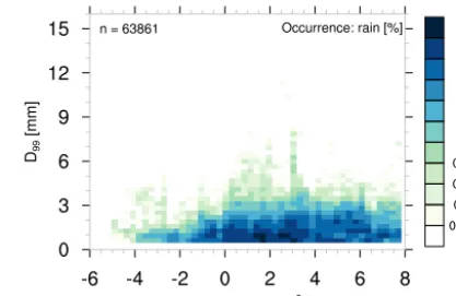
Figure 3. Two-dimensional histogram shows relative occurrence (%) for each PP (top: snow; middle: mixed phase; bottom: rain) after manual PP distinction from OceanRAIN RSM data set of RV Polarstern.ndenotes the number of minutes used per PP (165 632 in total).
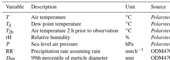
Atmospheric variables measured onboard RV Polarstern include temperature-related (T, Td, T2h) and humidity-related variables (rH, Td), air pressure (P), and, from the ODM470, wind speed (not used for analysis) and particle di-ameter (D). Instead ofD, we use the 99th percentile ofD,
D99, which is a measure for the maximum particle diameter measured within 1 min but excluding erroneously large parti-cles possibly caused by particle coincidences, drip-off drops, or other artifacts. Table 3 lists all relevant variables from RV Polarstern and the ODM470. Note that all variables are mea-sured distinctly higher than 2 m above the surface at about 43 m in order to reduce interfering sea spray and splashing wave water.
3 The automatic PP distinction
Table 3. List of available meteorological predictor variables in OceanRAIN used in the logistic regression model to predict the PP.
Variable Description Unit Source
T Air temperature ◦C Polarstern
Td Dew point temperature ◦C Polarstern
T2h Air temperature 2 h prior to observation ◦C Polarstern
rH Relative humidity % Polarstern
P Sea-level air pressure hPa Polarstern
RR Precipitation rate assuming rain mm h−1 ODM470 D99 99th percentile of particle diameter mm ODM470
Section 3.3 presents a novel approach that predicts three PPs applying two PP distributions (3P2D).
For the PP prediction we adopt a statistical model us-ing logistic regression to relate the available observed atmo-spheric variables (predictor variables) to the PP as suggested by Koistinen and Saltikoff (1998), henceforth KS98. The pre-dictor variables are fitted against binary dependent variables to calculate the PP probabilityp(PP). Taken from the manual PP distinction data (Sect. 2.2), the binary dependent variables attain a rain probabilityp(rain) [frac] of either 0 (snow) or 1 (rain). Once fitted,p(rain) can attain any value between 0 and 1 depending on the predictor variables.p(rain) is calculated by
p(rain)= 1
1+eα+β·V1+γ·V2+...+ω·Vn, (7)
whereby Vi represents the atmospheric predictor variables.
α,β,γ,. . .,ωdenote the regression coefficients that are de-termined by minimizing the sum of squared errors (nearest-neighbor method) with respect to the PPs from the manual PP distinction. Generally, we use the term PP probability,
p(PP), representing both rain (p(rain)) and snow probabil-ity (p(snow)) if not stated differently. The snow probability is calculated as 1−p(rain), excluding mixed phase for now in this simple model.
We calibrate various combinations of atmospheric predic-tor variables Vi (Table 3) for RS sub-data (Table 2) to find
the combination that predicts best the PP. KS98 state that the combination of air temperatureT and relative humidity rH, calledT_rH, is suited best to predict the PP. ForT_rH, Eq. (7) changes to
p(rain)= 1
1+e(α+β·T+γ·rH), (8)
where the number of regression coefficients reduces to three. In lack of alternative reference data, we evaluate the calcu-lated regression coefficients of RS sub-data using the same manually determined PPs as used for the model calibration. Nevertheless, we investigated the robustness of the regres-sion coefficients using 100 realizations of only 50 % ran-domly chosen minutes of precipitation from the RS data set. The standard deviation of the 100 realizations rarely exceeds
10 % of the individual regression coefficients from the whole RS data set, which confirms the robustness of the calcu-lated regression coefficients. If in the manual PP reference data set a minute of precipitation is assigned rain, the sta-tistical model by definition “agrees” forp(rain)≥0.5 while it “disagrees” for p(rain)<0.5. For the rain/snow distinc-tion four possible combinadistinc-tions exist – rain agreement, snow agreement, rain disagreement, and snow disagreement. For instance, rain disagreement means that the statistical model predicts rain that disagrees with the manual PP reference data indicating snow. Combined in a contingency table we choose four scores to evaluate how well the atmospheric predictor variable combinations serve to predict the PP in this statisti-cal model.
First, the accuracy serves to evaluate the overall correct-ness of the predictor variable combinations with respect to the manual PP reference data set. The accuracy represents the sum of cases in which model and manually determined PP reference data of RS sub-data agree divided by the total number of minutes in RS sub-data. Ideally, the accuracy is close to 1.
Second, we consider the bias score defined as the ratio be-tween the sum of disagreeing rain predictions and agreeing rain predictions to the sum of disagreeing snow predictions and agreeing rain predictions, all with respect to the manu-ally determined PP reference data. Accordingly, a bias score ofb <1 represents an overprediction of snow by the model, whereas b >1 represents an overprediction of rain by the model. However, the bias should be interpreted with cau-tion because the manual reference data set might be biased itself. Thus, the bias rather carries the information in which direction the predicted PP deviates from the manual refer-ence data.
Third, we determine the percentage of cases misclas-sified (PM). Misclasmisclas-sified means that predicted high-probability cases (p >0.95) disagree with the manual PP ref-erence data. For PM, the number of these misclassified cases is divided by the number of all RS cases. Ideally, PM is close to 0.
0.95 divided by all RS cases. Accordingly, PU measures the fraction of cases that the model is unable to predict at a high level of certainty. The definitions of PM and PU follow the evaluation method in Froidurot et al. (2014).
The four performance scores are calculated for both 100 realizations of 50 % randomly chosen minutes of precipita-tion (black boxes and whiskers in Fig. 4) and for all minutes of RS sub-data (red stars). The percentiles (5th, 25th, 50th, 75th, and 95th) illustrate how strongly the RS data set scatters and whether differences among predictor variable combina-tions are significant (p=0.95,n=100).
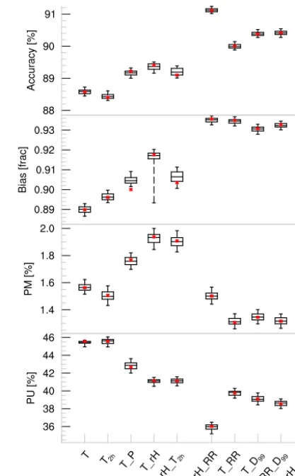
The PPs calculated with the logistic regression model reach an accuracy of more than 88 % for combinations of atmospheric predictor variables that all include the air tem-peratureT (Fig. 4).T carries the most straightforward PP in-formation in most cases. CombiningT with up to two other relevant predictor variables (connected by underscores) aids to assess their value in determining the PP. Table 4 displays the most important fitted regression coefficients for different combinations of predictor variables using the OceanRAIN sub-sample RS (2P1D) and the sub-sample RSM (3P1D and 3P2D).
Combining T with the air temperature 2 h prior to ob-servation (T2h) does not increase the accuracy of T (both 88.5 %). Other time intervals led to similarly small perfor-mance changes being in agreement with Froidurot et al. (2014). Accordingly, weather fronts associated withT drops do not seem to have an imprint on T_T2h or they are cur-rently underrepresented in the OceanRAIN data set. The air pressureP may have an impact on the PP at higher elevations due to lower air density (Dai, 2008). This, however, cannot explain the better accuracy of 89.2 % forT_P compared to
T. Over the ocean, the additional skill in the predictor P
might be caused by certain weather situations that favor ei-ther rain or snow, and are sufficiently sampled in the Ocean-RAIN data set. The relative humidity rH and the dew point
Td (not shown) reach about the same accuracy of 89.4 %. The addition ofP and rH toT leads to a statistically signifi-cant (p=0.95,n=100) but only slight increase in accuracy compared toT alone.
With the 99th percentile of the particle diameterD99and the calculated theoretical rain rate RR (Eqs. 3 and 4), phys-ical properties of precipitation particles directly enter the PP distinction. This direct physical relation explains the no-tably higher accuracy of at least 90 % byT_RR,T_D99, and other combinations containing RR and D99. The similarly high performance of these three predictor combinations is driven by the particle diameter that mainly influences RR. Combinations ofT, a humidity-related variable such as rH, and a diameter-related variable such asD99reach the high-est accuracy of more than 91 %. Combinations of four or five of the available atmospheric predictor variables such as
T_rH_RR_D99brought no noticeable further increase in ac-curacy (not shown). From the considered predictors, a
com-Figure 4. Box-and-whisker plot displays interquartile spread (black box: 25th, 50th, and 75th percentile) and lower (whisker: 5th per-centile) as well as upper (95th perper-centile) extremes, calculated from 100 realizations of each 50 % randomly chosen minutes of precip-itation from RS sub-data. Red stars denote the values for 100 % of RS sub-data. Accuracy (%), bias score (frac), percentage mis-classified (PM: fraction of disagreeing cases with high certainty of p >0.95 in %), and percentage unclassified (PU: fraction of uncer-tain cases of 0.05< p <0.95 in %) serve as performance scores using the calculated coefficients in Table 4 against the manually de-termined PP reference data. Labels indicate variable combinations, whereby all combinations includeT.
bination of three out of the available predictor variables suits best to accurately distinguish between rain and snow.
Table 4. List of regression coefficients calculated with Eq. (7) by minimizing the sum of squared errors with respect to the manual PP reference data for two PPs using one PP distribution (2P1D; Sect. 3.1), three PPs using one PP distribution (3P1D; Sect. 3.2), and three PPs using two PP distributions (3P2D; Sect. 3.3). For 3P2D, the asterisk denotes the rain distribution that was derived setting the mixed phase to snow. KS98 denotes the coefficients recommended by Koistinen and Saltikoff (1998) derived over Finland.
Method Variables used Regression coefficients (V1_V2_V3) α β γ δ
KS98 T_rH −22 2.7 0.2 – 2P1D T_rH −13.39 1.818 0.127 –
T_rH_D99 −10.83 1.780 0.118 −1.062
T_rH_RR −13.55 1.738 0.135 −0.325 3P1D T_rH −9.766 1.382 0.092 –
T_rH_D99 −8.364 1.364 0.090 −0.732
T_rH_RR −10.01 1.331 0.099 −0.204 3P2D T_rH −5.687 1.429 0.055 –
T_rH* −15.40 1.482 0.144 –
T_rH_D99 −4.794 1.467 0.056 −0.556
T_rH_D99* −13.94 1.431 0.145 −0.959
T_rH_RR −5.888 1.412 0.060 −0.059
T_rH_RR* −13.95 1.382 0.136 −0.316
Besides being accurate and unbiased, a small PP transition region of low PP certainty (low PU) combined with a low fraction of highly certain but misclassified PP cases (low PM) characterize a useful predictor variable combination. The PU decreases with increasing accuracy. Consequently, predictor variable combinations including rH and either D99 or RR reach the lowest PU of about 36 %. This low PU and thus fairly narrow PP distribution causes a slight increase in PM for T_rH_RR andT_rH_D99 (1.5 %) compared toT_D99,
T_RR, andT_RR_D99(1.3 %). However, the positive effect of using RR orD99outweighs the slightly negative influence of rH on PM. Consequently, the physical related predictor variables confirm their good performance in predicting the PP.
TheT_rH coefficients that were calculated for Finland in KS98 and confirmed in Froidurot et al. (2014) over Switzer-land reach an accuracy of 88.6 %, which is slightly lower than those coefficients optimized for OceanRAIN (89.4 %). A two-tailedt test confirms the difference to be statistically significant (p=0.99,n=100). The OceanRAIN-adapted coef-ficients exhibit a shallower rain/snow transition that results in a 0.8◦C lower temperature at p(rain)=0.1 while both distributions equal at p(rain)=0.9 (Fig. 5). Compared to OceanRAIN, the steeper rain/snow transition againstT fit-ted in KS98 holds a much lower PU of 24 % but to the ex-pense of a much higher PM of 4 % and a snow bias of 0.8. Consequently, the coefficients from KS98 better predict most uncertain cases withT_rH but miss more extreme cases such as freezing rain. For the OceanRAIN data set, the PP predic-tion using the RS-fitted coefficients better reflects the
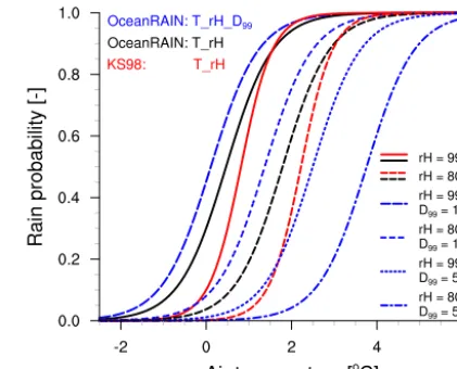
Ocean-Figure 5. Rain probability using regression coefficients from Ta-ble 4 for OceanRAIN RS sub-data (2P1D) with the predictor vari-ablesT_rH (black), T_rH_D99 (blue) both fitted against Ocean-RAIN, compared to KS98-recommended coefficients for T_rH (red). Dashed lines (black, red) indicate a PP distribution where rH is set to 80 % while for solid lines it is set to 99 %. ForT_rH_D99 (blue lines),D99is set to either 1 or 5 mm in addition to rH.
RAIN PP distribution compared to the KS98-fitted coeffi-cients as indicated by the accuracy.
ForT_rH_D99, the rain/snow transition shifts withT de-pending on D99. While D99=1 mm shifts the rain/snow transition to even lower temperatures by about 0.5◦C,D99= 5 mm shifts it towards higher temperatures by about 2◦C, both compared toT_rH derived from OceanRAIN RS sub-data. The shallower rain/snow transition of the PP distribu-tion fitted for OceanRAIN compared to that over Finland is likely caused by more freezing rain cases sampled in Ocean-RAIN, which the KS98-fitted coefficients forT_rH cannot predict.
3.2 One PP distribution to predict three PPs (3P1D) In a second step, we include mixed-phase precipitation into the algorithm because mixed-phase precipitation marks the transition from frozen to liquid particles and thus carries the highest uncertainty. We calculate the regression coef-ficients using the RSM sub-data including 165 632 min of precipitation measured onboard RV Polarstern. The three-phase distinction 3P1D fitsp(rain) against three PPs from the same manually determined PP reference data set as be-fore. However, the calculated transition phase between snow withp(rain)=0 and rain withp(rain)=1 is interpreted as mixed phase, defined in the range of 0.3≤p(rain)≤0.7 after KS98. The approximated coefficients for predictor variable combinationsVi differ considerably from those calculated
accuracy, bias, and PM serve as a measure of quality, while PU is no longer suitable for evaluation because the transition region of highest uncertainty between snow and rain rep-resents mixed-phase precipitation. Overall, this three-phase method 3P1D yields an accuracy between 74 and 78 %, which corresponds to an absolute decrease of about 14 % compared to 2P1D (Fig. 6). To that large decrease in accu-racy two reasons mainly contribute: (1) the manual PP refer-ence data, acting as referrefer-ence data, holds large uncertainties in the mixed phase, as well. The ww code represents snap-shots of 3-hourly observations. Therefore, they hardly satisfy the need for minute-based observations because the mixed-phase rain/snow fraction can vary dramatically, both tempo-rally and spatially. (2) KS98 assume the mixed-phase pre-cipitation to occur in the transition region between rain and snow, which is true in most cases. However, several cases exist in which mixed-phase precipitation occurs at distinctly high or low air temperature (Fig. 3) and thus 3P1D misclas-sifies these cases.
Relative to each other, the individual variable combina-tions perform similar compared to 2P1D. T, T_T2h, and
T_P have the lowest accuracy of below 75 % (Fig. 6) and a bias below 0.92. The addition of rH significantly increases the accuracy by about 1 %, whereas T_rH_T2h,
T_rH, andT_Td_T2h (not shown) do not differ much from each other. The predictor variable combinations that include the diameter-related predictors RR andD99lead to the high-est accuracy of 76 up to 78 %. The highhigh-est accuracy of 78 % reached by T_rH_D99 represents a statistically significant performance increase to the remaining variable combinations in 3P1D, which contrasts to 2P1D whereT_rH_RR does not perform significantly better thanT_rH_D99.
For the bias, predictor combinations including RR and/or
D99 reach the least pronounced snow bias of about 0.93, whereas the remaining predictor combinations feature signif-icantly lower biases, mostly below 0.92. In that respect, the bias of 3P1D resembles that of 2P1D (see Fig. 4 in Sect. 3.1) both in terms of magnitude and in the individual performance of the predictor variable combinations.
While the ranking of predictor variable combinations with respect to accuracy and bias looks very similar compared to 2P1D, PM tends to form three clusters. The first cluster com-prises predictor variables without particle diameter informa-tion, holding the lowest PM of 2.2 to 2.4 %. The second clus-ter includes RR but notD99, holding the highest PM (3.4 %). In the third cluster each predictor variable combination in-cludesD99 but performs better than the second cluster with PM of about 2.8 %.T_rH_D99in the third cluster offers the best compromise in maximizing the accuracy while minimiz-ing the fraction of misclassified cases.
In contrast to 2P1D, for 3P1D PM tends to scale with accuracy for many predictor variable combinations. While
T_rH_D99 exhibits an about 0.5 % larger PM thanT, the PM of T_rH_RR andT_RR are even 1.1 % larger. A high PM indicates a clear disagreement between calculated PP
Figure 6. Performance of fit is shown for different combinations of atmospheric variables as in Fig. 4 for RSM sub-data. All variable combinations again includeT.
and manually estimated PP. Note, however, that not in all of these clearly disagreeing cases the manual PP reference data necessarily contains the correct PP. Physically related pre-dictor variables such asD99can assist to unveil cases falsely classified by the manual PP estimation. For example,D99is able to identify snow or mixed-phase cases, falsely classi-fied as rain in the manual reference data. Except for the trop-ics, rain drops rarely exceed drop diameters of 5 mm (Bent-ley, 1904; Villermaux and Bossa, 2009). Larger drops mainly break up or collide with neighboring drops.D99excludes co-incidences of drops as well as artificial drops dripping off the instrument housing by discarding the uppermost percentile of measured drop diameters per minute. Therefore, particles classified as rain drops withD99>5 mm very likely represent frozen particles, which means that they were falsely classi-fied as rain (Fig. 7). Below 4◦C, 163 rain cases in RSM sub-data (about 0.25 %) are likely falsely classified. This could explain about half of the 0.5 % PM difference ofT_rH_D99 toT in Fig. 6).
cannot represent the temperature distribution of PPs in the OceanRAIN data set.
3.3 Two PP distributions to predict three PPs (3P2D) The relatively low accuracy reached with the three-phase method after KS98 using one PP distribution (3P1D) moti-vates a novel investigation of how to further improve the PP prediction for three PPs. Instead of applying one PP distribu-tion to determine rain, mixed-phase, and snow precipitadistribu-tion, we suggest to approximate two separate PP distributions for rain and snow (3P2D). These two individual PP distributions are derived analogous to the method for one PP distribution by assigning the mixed-phase PP differently – first set it to rain to calculate the snow PP distribution, then set it to snow to calculate the rain PP distribution. Subtracting the sum of both individually calculated PP distributions from 1 yields the PP distribution for mixed phase. In contrast to 3P1D, the separately calculated coefficients for rain and snow (Table 4) lead to individual distributions only connected via the mixed phase.
Analogous to 2P1D (Sect. 3.1), the accuracy represents the percentage of cases withp(PP)>0.5 that agree in their respective PP with the manual PP reference data. The bias represents the ratio between the sum of predicted rain cases and the sum of rain cases in the manual PP reference data. Please note that the bias definition remains unchanged for 3P2D that includes mixed phase compared to 2P1D. How-ever, the additional PP distribution slightly modifies the cal-culation of PM and PU, illustrated in Fig. 8. PM represents the percentage of all certain cases (p(PP)>0.95; hatched area in Fig. 8) in which either one of the PPs disagrees with the manual PP reference data. PU as the percentage of un-certain cases (0.05< p(PP)<0.95; shaded area) represents only those cases where all PPs are uncertain after definition. We introduce this limitation because ifp(PP)<0.05 holds for at least one PP then we would not consider this PP uncer-tain anymore. Note that for mathematical reasons we cannot display PMmix>0 and PU>0 in the same figure, which is why we set PMmix>0.
This 3P2D method using two individual PP distributions reaches on average a higher accuracy compared to 3P1D (Fig. 9). Whereas T,T_T2h, and T_P hold less than 78 % accuracy,T_rH_D99reaches the highest accuracy of 81.2 %. As for 3P1D, the improvement is mainly caused by adding the predictorD99that performs significantly better than when adding the predictor RR. Also the overprediction of snow by all predictor variable combinations with respect to the man-ually determined PP reference data stays the same in 3P2D. The physically related variables are least biased (about 0.93), which consistently highlights the improvement of including them in the predictor variable combination. However, for PM stronger differences among these physically related predic-tor variables arise. WhileT_RR holds the highest PM (about 2.3 %), T_rH_D99 reaches 1.9 % PM, which is on the
or-Figure 7. Two-dimensional histogram of temperature and the 99th percentile of the particle diameter for cases classified as rain by the manual PP estimation in RSM.
der of the predictor variable combinations without RR and
D99(1.8 %). However, the physically related predictors reach again lowest PUs of about 38 % while T holds a PU of 51 %. In combination with the other scores we recommend
T_rH_D99 followed byT_RR_D99 andT_D99to most ac-curately predict the PP using two independent PP distribu-tions.
Compared to 3P1D after KS98, the PM decreases for 3P2D. This decrease in PM ranges between 0.5 and 1 % and thus highlights the improved performance of using two PP distributions instead of one to predict the PP. The lower PM and higher accuracy approve that the novel method apply-ing two independent PP distributions better represents the PP distribution in OceanRAIN RSM.
To understand the better performance of 3P2D com-pared to 3P1D after KS98, we consider how the PP frac-tion is distributed with respect to T around the freezing point (rain/snow transition) in the manual PP reference data (Fig. 10). While the rain occurrence shows a relatively low skewness, the mixed-phase/snow distribution is slightly left-skewed. This higher skewness with a secondary maximum in the mixed-phase distribution at−3◦C (minimum in snow distribution) cannot be well represented by one PP distribu-tion. One PP distribution is limited to match all three PP dis-tributions at the same time that can only represent an average skewness. In that respect, deriving two independent PP dis-tributions driven by mixed-phase precipitation better reflects the PP distribution of each PP individually with respect to the manual PP reference data in OceanRAIN RSM.
Figure 8. Graph illustrates the calculation of PU (framed) and PM (hatched) including snow (dashed/purple), mixed phase (dot-ted/orange), and rain (solid/cyan), analogous to Fig. 3 in Froidurot et al. (2014). PU divides the sum of cases with 0.05< p(PP)<0.95 for all PPs by the sum of all RSM cases. PM divides the sum of cases withp(PP)>0.95 for one of the PPs that disagrees with the manual PP estimation by the sum of all RSM cases. We set PMmix>0 be-cause otherwise we could not display it in the same PP distribution (rH kept constant) with PU>0.
aspect by reanalyzing the constantly growing OceanRAIN database.
Nevertheless, differences remain due to the chosen PP distinction method. By discriminating three PPs, 3P1D and 3P2D enable a smoother rain/snow transition compared to 2P1D due to included mixed-phase precipitation (Fig. 11). At lower temperatures, 2P1D approaches the snow distribu-tion of 3P2D, while at higher temperatures it approaches the rain distribution of 3P2D. In other words, the steeper rain probability distribution for 2P1D clarifies the slightly smaller unclassified range (0.3< p(PP)<0.7) compared to 3P2D as seen in the percentage unclassified (compare Fig. 4 and Fig. 9).
D99 as additional variable inT_rH_D99 tends to shift the snow and rain distributions to higher temperatures and apart of each other, which also resolves more extreme cases. This distribution shift with temperature follows a physical reason: large snow particles better withstand melting at high air tem-peratures than small snow particles. This physical informa-tion lacks inT_rH, which notably decreases its accuracy (cf. Fig. 9).
4 Discussion
After finding suitable methods for both the rain/snow distinc-tion (Sect. 3.1) as well as for the rain/snow/mixed-phase dis-tinction (Sect. 3.3) we compare the results to those of similar studies. For the rain/snow distinction over Switzerland us-ingT_rH derived over Finland by KS98, Schmid and Mathis
Figure 9. As Fig. 4 but for RSM including mixed phase, using two independent PP distributions (3P2D). The calculation of PM and PU differs from Fig. 4 as displayed and explained in Fig. 8.
(2004) find a higher accuracy of 92.4 % compared to our cal-culated accuracy of 88.6 % when using the same KS98 re-gression coefficientsα=22,β=2.7,γ =0.2. Schmid and Mathis (2004) find an overprediction of snow cases (bias 0.82), very similar to the OceanRAIN RS snow overpredic-tion (bias 0.8) using the same coefficients derived by KS98. However, for fitting the regression coefficients to our data set (Table 4) we still obtain a slightly lower accuracy of 89.4 % calculated forT_rH and 91 % forT_rH_D99 while the low-bias decreases to 0.92 and 0.93, respectively. These perfor-mance improvements indicate, first, different conditions for PP transition over the ocean compared to Finland of KS98 while, second, the OceanRAIN data set is in relatively close agreement with the Swiss data.
Figure 10. Lines show PP fraction for rain (solid, cyan), mixed phase (dotted, orange), and snow (purple, dashed) from Ocean-RAIN RSM (165 632 min) determined with the manual PP estima-tion against temperature. Gray bars represent the temperature fre-quency of occurrence (in 103).
Figure 11. Air temperature versus predicted PP by the different methods: two PPs (2P1D; solid blue), three one-PP distributions (3P1D; dashed red), and three two-PP distributions (3P2D; dot-ted black). 3P2D consists of two curves (left: snow distribution as 1−p(snow); right: rain distribution asp(rain)) for the calculated coefficients ofT_rH_D99(left panel; rH=85 %,D99=5 mm) and T_rH (right panel; rH=85 %).
winter period) and 85 % compared to independent climato-logical stations over Norway (1 month). They obtain an over-prediction of snow (bias of 0.92) and problems in predict-ing the PP of supercooled rain durpredict-ing prevailpredict-ing tempera-ture inversions. In OceanRAIN we find a similar overpredic-tion of snow (bias T_rH: 0.91; T_rH_D99: 0.93) with re-spect to the manual PP reference data in OceanRAIN. This overprediction of snow occurs predominantly around 0◦C that is the temperature range sampled most frequently (cf. Fig. 10). Hence, OceanRAIN is likely to face the same prob-lems underpredicting rain when supercooled raindrops fall
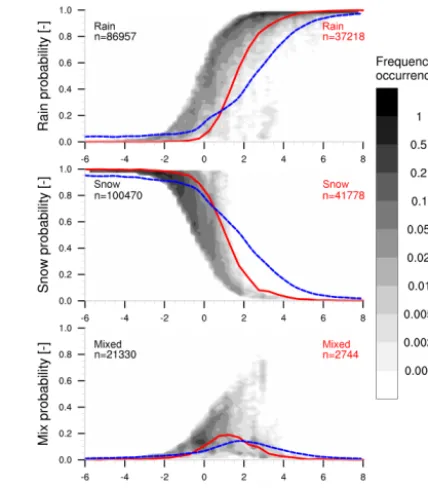
Figure 12. PP probability shown using the new 3P2D method with two individual PP distributions (T_rH_D99) as frequency of occur-rence (%) in gray shades against air temperature according to PP reference data that separates rain, snow, and mixed phase in Ocean-RAIN ALL for more than 4 years of RV Polarstern data. Solid red lines represent the mean PP fraction from observations in the Swiss Alps (1991–2010) from Froidurot et al. (2014); dashed blue lines show mean PP fraction for oceanic ship data (DS464.0; 1977–2007) from Dai (2008).
under prevailing temperature inversions. Further work is re-quired in order to clarify whether we need additional ancil-lary data to reduce the bias or whether the logistic regression model is unable to provide a less biased PP prediction.
Assuming that mixed-phase precipitation causes most of the accuracy decrease between 2P1D and 3P1D as well as 3P2D, we consider the individual probability of detec-tion (POD) for rain, snow, and mixed phase. For rain, the POD is calculated by dividing the number of agreeing rain cases by the number of all observed rain cases. For the POD of 3P1D using the KS98-fitted coefficients forT_rH for rain, snow, and mixed phase we find 0.92, 0.78, and 0.21 (T_rH_D99: 0.92, 0.86, and 0.25). The respective PODs from Gjertsen and Ødegaard (2005) for the same settings re-veal slightly different PODs of 0.81, 0.97, and 0.25. Whereas they obtain a notably higher POD for snow, the rain POD is lower compared to OceanRAIN. Nevertheless, mixed-phase precipitation confirms to carry the largest prediction uncer-tainty of all three PPs.
(2014), in most cases the PP transition in OceanRAIN oc-curs at lower temperatures (Fig. 12). However, the analysis by Froidurot et al. (2014), among other conditions, neglects all kinds of freezing rain (ww=56,57,66,67) that we as-sign to rain. Without these “cold rain” cases, the rain/snow transition shifts towards higher temperature that may in parts explain the temperature difference in Fig. 12. Additionally, the PP probability distribution in the OceanRAIN RV Po-larstern data sample is biased by the high number of temper-atures around 0◦C that occur by a factor of 3 to 4 more often than temperatures between −4 and 4◦C (cf. Fig. 10), and relative humidity close to 100 %. These frequently sampled conditions put their mark on the average rain/snow transi-tion by reducing the rain/snow transitransi-tion temperature com-pared to the Swiss Alps where T and rH were sampled more homogeneously (Fig. 9 in Froidurot et al., 2014). De-spite the high number of available minutes with precipita-tion in OceanRAIN, the rather short time series on climato-logical timescales and the spatial distribution of along-track data limit the representativeness. However, a different land– ocean rain/snow transition might be observable. Dai (2008) found a systematic land–ocean difference in the rain/snow transition between land and ocean in 30 years of NCEP ADP Operational Global Surface Observations (DS464.0; 1977–2007). Whereas over land, rain transitions into snow relatively quickly (−2< T <4◦C), over ocean the transi-tion zone is wider (−3< T <6◦C). Although the rain/snow transition zone within OceanRAIN appears wider compared to regression coefficients recommended by Koistinen and Saltikoff (1998) as seen in Fig. 5, the rain/snow transi-tion in OceanRAIN compares better to the Swiss Alps data (Froidurot et al., 2014) than to the NCEP DS464.0 ocean data (Dai, 2008) that reveal a wider transition zone. In spe-cific, OceanRAIN relatively closely agrees with the NCEP DS464.0 ocean data forT <0◦C, whereas larger differences of>1◦C occur in the range of 2< T <5◦C. Two main rea-sons can explain the different rain/snow transitions between OceanRAIN and NCEP DS464.0 ocean data by Dai (2008). (1) ww codes used in the NCEP ocean data are subject to larger uncertainty compared to OceanRAIN. In contrast to the RV Polarstern onboard weather observatory by the Ger-man Meteorological Service, Ger-many VOSs such as cargo ships in NCEP DS464.0 ocean data have inadequately trained ob-servers that might use certain ww codes preferentially, ships possibly avoid bad weather, or measurement quality may suf-fer from instrument biases (Petty, 1995). For these reasons, the wider rain/snow transition zone likely reflects a higher uncertainty of the NCEP DS464.0 ocean data compared to the OceanRAIN data from RV Polarstern or the Swiss Alps data. (2) RV Polarstern mainly sampled warm-season pre-cipitation in the Atlantic Arctic and Antarctic regions with the exception of the austral cold season in 2013. In addi-tion to that, the heterogeneous regional and seasonal sam-pling by RV Polarstern might have favored conditions under which inversions prevail that allow rain at fairly low
temper-atures but inhibit snow under relatively high tempertemper-atures. While the sampling imbalance of RV Polarstern may indi-cate a restricted representativeness of PPs in OceanRAIN, theT_rH_D99predictor variable combination recommended as the new automatic PP distinction method for OceanRAIN well represents the observed PPs within OceanRAIN. The continuously growing time series of RV Polarstern among other RVs in OceanRAIN allows to recalibrate or refine the algorithm geographically for a longer time series with com-prehensive statistical sampling in the future.
5 Summary and concluding remarks
We developed a novel automatic algorithm to distinguish the PP within OceanRAIN in situ precipitation data to in-troduce a statistical PP probability and to increase the data post-processing efficiency. The analysis focused on identify-ing the most suitable combination of available atmospheric predictor variables to determine the PP. For that purpose, we applied a simple logistic regression model suggested by Koistinen and Saltikoff (1998) that was shown to perform well over land. Previous studies mainly rely on air temper-atureT, relative humidity rH, air pressureP, and others to predict the PP. We investigated several of these atmospheric predictor variable combinations to obtain a PP probability. In particular, we tested the performance of the logistic regres-sion model after Koistinen and Saltikoff (1998) for Ocean-RAIN using two (excl. mixed phase) and three PPs (incl. mixed phase) against the manually estimated observation-based PP in OceanRAIN. Besides increasing the efficiency in predicting the PP with an automatic method, we developed a novel three-phase method that uses two individual and inde-pendent PP distributions to predict the PP more accurately.
The study led to the following main results.
a. In OceanRAIN, the combination of air temperatureT, relative humidity rH, and the 99th percentile of the par-ticle diameterD99(calledT_rH_D99) predicts best the PP for all investigated methods.
b. Applying more than three of the chosen atmospheric predictor variables negligibly increases the accuracy in predicting the PP.
c. The two-phase method (2P1D) using the predictor vari-able combinationT_rH_D99and regression coefficients fitted to OceanRAIN reaches an accuracy above 91 % with a slight overestimation of snow cases for the mid-and high latitudes between−6 and 8◦C in the Ocean-RAIN data set with respect to the manual PP reference data including shipboard present weather observations. d. A novel three-phase method using two individual PP
1998). As a reason, two individual PP distributions are capable of better representing unequally distributed or skewed PP distributions of atmospheric predictor vari-ables as well as certain weather situations that might currently be over- or undersampled. Accordingly, this performance difference might decrease once the inves-tigated 4-year OceanRAIN time series grows further while sampling biases vanish.
e. The OceanRAIN data using 3P2D reveal a wider rain/snow transition zone compared to data derived over Finland (Koistinen and Saltikoff, 1998). The rain/snow transition in OceanRAIN occurs at slightly lower tem-peratures compared to the data from Finland as well as NCEP DS464.0 global ocean ship data (Dai, 2008). The difference in the rain/snow transition zone likely origi-nates from heterogeneous spatial and seasonal sampling in OceanRAIN that is likely to decrease with an increas-ing OceanRAIN time series. In contrast, a higher quality of the derived ww codes in OceanRAIN compared to the average VOS suggests a higher certainty of the derived PPs. The Swiss Alps data (Froidurot et al., 2014) shows a similar rain/snow transition at slightly higher tempera-tures, likely caused by neglected cases of freezing rain, among others. Due to these differences we obtain the highest accuracy and lowest bias when applying regres-sion coefficients fitted to the OceanRAIN data set in-stead of using recommended coefficients from the liter-ature such as those from Koistinen and Saltikoff (1998). f. The new PP distinction algorithm 3P2D includingD99 as essential physical information identified several cases that were erroneously classified as rain within the man-ual PP estimation. Large particle diameters indicate that the PP should be classified as snow or at least mixed-phase precipitation instead of rain.
g. Mixed-phase precipitation carries the largest uncer-tainty of the three PPs and is most challenging to detect for the new algorithm with a probability of detection of up to 0.25 using the predictor variable combination
T_rH_D99and 3P2D.
Even though the newly developed automatic PP distinction algorithm strongly depends on the currently still limited OceanRAIN data set, remarkable improvements are made. First, a PP probability is provided on a minute basis that lim-its the number of highly uncertain cases requiring visual in-spection of atmospheric variables. The PP probability further allows error characterizing other precipitation data sets such as satellite data using OceanRAIN precipitation rates to un-veil systematic errors with respect to PP. Second, the PPs of a few critical cases could be corrected that were falsely clas-sified by the manual method. Third, we give evidence that the particle diameter of the falling precipitation particles con-tributes valuable information to the PP separation and by that
in a physical way significantly improves the algorithm accu-racy. Fourth, the new PP distinction algorithm considerably speeds up the data processing within OceanRAIN, which is an important step towards a fast-growing global surface pre-cipitation data set for validating and evaluating other oceanic precipitation data sets.
Data availability
The OceanRAIN data set is publicly available upon request free of charge. A registration with a digital object identi-fier is planned. Further information are available on http: //oceanrain.org.
Acknowledgements. We would like to thank the crew of RV Polarstern including the German Meteorological Service and the Alfred Wegener Institute for their support and assistance in supervising the instrument and caring for a smooth operation and ship-board access. We further thank Nicole Albern for carefully processing the data. Helpful comments by Bjorn Stevens are well appreciated to finalize the manuscript. We also like to thank two anonymous reviewers for their valuable comments. We acknowl-edge the financial support of the German Research Foundation in research unit FOR1740.
The article processing charges for this open-access publication were covered by the Max Planck Society.
Edited by: M. Kulie
References
Adler, R. F., Gu, G., and Huffman, G. J.: Estimating Clima-tological Bias Errors for the Global Precipitation Climatol-ogy Project (GPCP), J. Appl. Meteorol. Clim., 51, 84–99, doi:10.1175/JAMC-D-11-052.1, 2012.
Atlas, D. and Ulbrich, C.: The physical basis for attenuation-rainfall relationships and the measurement of rainfall parameters by combined attenuation and radar methods, J. Rech. Atmos., 8, 275–298, 1974.
Battaglia, A., Rustemeier, E., Tokay, A., Blahak, U., and Simmer, C.: PARSIVEL Snow Observations: A Crit-ical Assessment, J. Atmos. Ocean. Tech., 27, 333–344, doi:10.1175/2009JTECHA1332.1, 2010.
Bentley, W.: Studies of Raindrops and Raindrop Phenom-ena, Mon. Weather Rev., 32, 450–456, doi:10.1175/1520-0493(1904)32<450:SORARP>2.0.CO;2, 1904.
Bumke, K. and Seltmann, J.: Analysis of Measured Drop Size Spectra over Land and Sea, ISRN Meteorology, 2012, 1–10, doi:10.5402/2012/296575, 2012.
Dai, A.: Temperature and pressure dependence of the rain-snow phase transition over land and ocean, Geophys. Res. Lett., 35, L12802, doi:10.1029/2008GL033295, 2008.
Friedrich, K., Higgins, S., Masters, F. J., and Lopez, C. R.: Artic-ulating and Stationary PARSIVEL Disdrometer Measurements in Conditions with Strong Winds and Heavy Rainfall, J. At-mos. Ocean. Tech., 30, 2063–2080, doi:10.1175/JTECH-D-12-00254.1, 2013.
Froidurot, S., Zin, I., Hingray, B., and Gautheron, A.: Sensi-tivity of Precipitation Phase over the Swiss Alps to Differ-ent Meteorological Variables, J. Hydrometeorol., 15, 685–696, doi:10.1175/JHM-D-13-073.1, 2014.
Fuchs, T., Rapp, J., Rubel, F., and Rudolf, B.: Correction of synop-tic precipitation observations due to systemasynop-tic measuring errors with special regard to precipitation phases, Phys. Chem. Earth Pt. B, 26, 689–693, doi:10.1016/S1464-1909(01)00070-3, 2001. Gjertsen, U. and Ødegaard, V.: The water phase of precipitation –
a comparison between observed, estimated and predicted values, Atmos. Res., 77, 218–231, doi:10.1016/j.atmosres.2004.10.030, 2005.
Goodison, B. E.: Accuracy of Canadian Snow Gage Measure-ments, J. Appl. Meteorol., 17, 1542–1548, doi:10.1175/1520-0450(1978)017<1542:AOCSGM>2.0.CO;2, 1978.
Großklaus, M.: Niederschlagsmessung auf dem Ozean von fahren-den Schiffen, PhD thesis, Institut für Meereskunde, Christian-Albrechts-Universität Kiel, Kiel, Germany, 1996.
Hogan, A. W.: Objective Estimates of Airborne Snow Proper-ties, J. Atmos. Ocean. Tech., 11, 432–444, doi:10.1175/1520-0426(1994)011<0432:OEOASP>2.0.CO;2, 1994.
Ishizaka, M., Motoyoshi, H., Nakai, S., Shiina, T., Kumakura, T., and Muramoto, K.-i.: A New Method for Identifying the Main Type of Solid Hydrometeors Contributing to Snowfall from Mea-sured Size-Fall Speed Relationship, J. Meteorol. Soc. Jpn., 91, 747–762, doi:10.2151/jmsj.2013-602, 2013.
Kent, E. C., Ball, G., Berry, D. I., Fletcher, J., Hall, A., North, S., and Woodruff, S.: The Voluntary Observ-ing Ship (VOS) Scheme, European Space Agency, 518–528 doi:10.5270/OceanObs09.cwp.48, 2010.
Kidd, C. and Levizzani, V.: Status of satellite precipita-tion retrievals, Hydrol. Earth Syst. Sci., 15, 1109–1116, doi:10.5194/hess-15-1109-2011, 2011.
Klepp, C.: The oceanic shipboard precipitation measurement net-work for surface validation – OceanRAIN, Atmos. Res., 163, 74–90, doi:10.1016/j.atmosres.2014.12.014, 2015.
Klepp, C., Bumke, K., Bakan, S., and Bauer, P.: Ground vali-dation of oceanic snowfall detection in satellite climatologies during LOFZY, Tellus A, 62, 469–480, doi:10.1111/j.1600-0870.2010.00459.x, 2010.
Koistinen, J. and Saltikoff, E.: Eperience of customer products of accumulated snow, sleet and rain, COST75 Advanced Weather Radar Systems, 1998.
Lanza, L. G. and Vuerich, E.: The WMO Field Intercompar-ison of Rain Intensity Gauges, Atmos. Res., 94, 534–543, doi:10.1016/j.atmosres.2009.06.012, 2009.
Lempio, G. E., Bumke, K., and Macke, A.: Measurement of solid precipitation with an optical disdrometer, Adv. Geosci., 10, 91– 97, doi:10.5194/adgeo-10-91-2007, 2007.
Löffler-Mang, M. and Joss, J.: An Optical Disdrometer for Measuring Size and Velocity of Hydrometeors, J. Atmos. Ocean. Tech., 17, 130–139, doi:10.1175/1520-0426(2000)017<0130:AODFMS>2.0.CO;2, 2000.
Merenti-Välimäki, H.-L., Lönnqvist, J., and Laininen, P.: Present weather: comparing human observations and one type of automated sensor, Meteorol. Appl., 8, 491–496, doi:10.1017/S1350482701004108, 2001.
Michelson, D. B.: Systematic correction of precipitation gauge ob-servations using analyzed meteorological variables, J. Hydrol., 290, 161–177, doi:10.1016/j.jhydrol.2003.10.005, 2004. Ocean Rainfall And Ice phase precipitation measurement Network
(OceanRAIN): precipitation particle spectra, precipitation rates and ancillary data from RV Polarstern over the Atlantic Ocean in-cluding polar regions, University Hamburg, CliSAP/CEN, Ham-burg, Germany, available at: http://oceanrain.org, last access: 7 April 2016.
Petty, G. W.: Frequencies and Characteristics of Global Oceanic Precipitation from Shipboard Present-Weather Reports, B. Am. Meteorol. Soc., 76, 1593–1616, doi:10.1175/1520-0477(1995)076<1593:FACOGO>2.0.CO;2, 1995.
Schmid, W. and Mathis, A.: Validation of methods to detect winter precipitation and retrieve precipitation type, 12th SIRWEC Con-ference, 16–18 June 2004, Bingen, Germany, 2004.
Schneider, U., Becker, A., Finger, P., Meyer-Christoffer, A., Ziese, M., and Rudolf, B.: GPCC’s new land surface precipitation cli-matology based on quality-controlled in situ data and its role in quantifying the global water cycle, Theor. Appl. Climatol., 115, 15–40, doi:10.1007/s00704-013-0860-x, 2014.
Taylor, P.: Intercomparison and Validation of Ocean-Atmosphere Energy Flux Fields – Final report of the Joint WCRP/SCOR Working Group on Air-Sea Fluxes, 325 pp., WCRP-112, WMO/TD-1036, 2000.
Villermaux, E. and Bossa, B.: Single-drop fragmentation deter-mines size distribution of raindrops, Nat. Phys., 5, 697–702, doi:10.1038/nphys1340, 2009.
Weller, R. A., Bradley, E. F., Edson, J. B., Fairall, C. W., Brooks, I., Yelland, M. J., and Pascal, R. W.: Sensors for physical fluxes at the sea surface: energy, heat, water, salt, Ocean Sci., 4, 247–263, doi:10.5194/os-4-247-2008, 2008.
WMO: Code Tables and Flag Tables Associated with BUFR/CREX Table B, available at: http://www.wmo.int/pages/prog/www/ WMOCodes/WMO306_vI2/LatestVERSION/WMO306_vI2_ BUFRCREX_CodeFlag_en.pdf (last access: 7 April 2016), 2015.
Yuter, S. E. and Parker, W. S.: Rainfall Measurement on Ship Revisited: The 1997 PACS TEPPS Cruise, J. Appl. Meteorol., 40, 1003–1018, doi:10.1175/1520-0450(2001)040<1003:RMOSRT>2.0.CO;2, 2001.