Scaling and multifractal fields in the solid earth and topography

Nonlin. Processes Geophys., 14, 465–502, 2007 www.nonlin-processes-geophys.net/14/465/2007/ © Author(s) 2007. This work is licensed

under a Creative Commons License.

Nonlinear Processes

in Geophysics

Scaling and multifractal fields in the solid earth and topography

S. Lovejoy1,2and D. Schertzer3,4

1_{Physics, McGill University, 3600 University st., Montreal, Que. H3A 2T8, Canada} 2_{GEOTOP UQAM/McGill Center, Montreal, Qc, Canada}

3_{CEREVE, Ecole Nationale des Ponts et Chauss´ees, 6–8, avenue Blaise Pascal, Cit´e Descartes, 77455 Marne-La-Vallee}

Cedex, France

4_{Meteo France, 1 Quai Branly, 75007 Paris, France}

Received: 29 March 2007 – Revised: 4 July 2007 – Accepted: 4 July 2007 – Published: 2 August 2007

Abstract. Starting about thirty years ago, new ideas in non-linear dynamics, particularly fractals and scaling, provoked an explosive growth of research both in modeling and in ex-perimentally characterizing geosystems over wide ranges of scale. In this review we focus on scaling advances in solid earth geophysics including the topography. To reduce the review to manageable proportions, we restrict our attention to scaling fields, i.e. to the discussion of intensive quantities such as ore concentrations, rock densities, susceptibilities, and magnetic and gravitational fields.

We discuss the growing body of evidence showing that geofields are scaling (have power law dependencies on spa-tial scale, resolution), over wide ranges of both horizontal and vertical scale. Focusing on the cases where both hori-zontal and vertical statistics have both been estimated from proximate data, we argue that the exponents are systemati-cally different, reflecting lithospheric stratification which – while very strong at small scales – becomes less and less pronounced at larger and larger scales, but in a scaling man-ner. We then discuss the necessity for treating the fields as multifractals rather than monofractals, the latter being too re-strictive a framework. We discuss the consequences of multi-fractality for geostatistics, we then discuss cascade processes in which the same dynamical mechanism repeats scale af-ter scale over a range. Using the binomial model first pro-posed by de Wijs (1951) as an example, we discuss the issues of microcanonical versus canonical conservation, algebraic (“Pareto”) versus long tailed (e.g. lognormal) distributions, multifractal universality, conservative and nonconservative multifractal processes, codimension versus dimension for-malisms. We compare and contrast different scaling models (fractional Brownian motion, fractional Levy motion, con-tinuous (in scale) cascades), showing that they are all based on fractional integrations of noises built up from singularity

Correspondence to: S. Lovejoy

([email protected])

basis functions. We show how anisotropic (including strati-fied) models can be produced simply by replacing the usual distance function by an anisotropic scale function, hence by replacing isotropic singularities by anisotropic ones.

1 Introduction

466 S. Lovejoy and D. Schertzer: Multifractals and the solid earth of the earth’s topography was of the “remarkable” scaling

formk−β with spectral exponentβ=2; close to the modern valueβ≈2.1 (kis a wavenumber, see below for discussion), and de Wijs (1951) who – for the distribution of ores – first suggested an explicit cascade model.

Until Mandelbrot (1977)’s seminal “Fractals: form, chance and dimension” these pioneering papers were iso-lated. However, the 1970s were a period of explosive growth of nonlinear dynamics, particularly after the discovery by Feigenbaum (1978) and others of quantitative universality in deterministic chaos: the geoscience community was primed for new ideas. In this context, and riding on the back of the computer graphics revolution, Mandelbrot’s proposal that fractals are ubiquitous in nature struck a responsive chord. It promised to characterize and model many of the messy prob-lems of geocomplexity using unique fractal dimensions.

When it came to geophysical applications, this audacious idea turned out to have serious limitations: most geofields of interest are mathematical fields (i.e. they have a value at each space-time point such as the atmospheric temperature or rock density), and – in spite of many attempts – they can-not be reduced to geometric sets of points. They therefore cannot generally be characterized by unique fractal dimen-sions. Furthermore, the proposed fractal sets were only scale invariant under isotropic scale changes or occasionally under the slightly more general “self-affine” scale changes in which different exponents act in different orthogonal directions.

Since Mandelbrot’s original proposal of applying fractal geometry to natural systems, geoscience applications – espe-cially in turbulence – played an important role in stimulating advances. There are four key developments on which we focus here. The first is the realization that a generic conse-quence of scale invariant dynamics – where the same basic mechanism repeats scale after scale from large to small – are multifractal fields i.e. it requires the transition from fractal geometry to multifractal processes. In these “cascades”, the variability is built up scale after scale; the generic result is that the extremes are particularly singular, they display “di-vergence of moments” or equivalently algebraic/power law (“Pareto”) distributions (also called the “multifractal but-terfly effect” (Lovejoy and Schertzer, 1998)). Since Bak et al. (1987, 1988), the combination of fractals combined with algebraic probabilities has been termed “Self-Organized Criticality” (SOC), therefore cascades can be said to pro-vide an alternative nonclassical “multifractal phase transi-tion” route to SOC (Schertzer and Lovejoy, 1994). The third advance was the realization that when – over a finite range of scales – such a scaling process interacts with many others or is iterated enough, that the resulting behaviour is stable and attractive. This implies that it doesn’t depend on many of the details of the dynamics; i.e. that there exist “univer-sality classes” for multifractal processes. This essentially re-duces the number of exponents from infinity to only three and finally allows multifractals to be manageable. This is a kind of multiplicative central limit theorem. The fourth key

advance was the recognition that scale invariance is a very general (although nonclassical) symmetry principle. The de-velopment of this “Generalized Scale Invariance” (GSI) ef-fectively extended scale invariance from the restrictive and unrealistic isotropic (“self-similar”) fractals and multifrac-tals to highly anisotropic systems. In scaling but anisotropic systems, as one “zooms” into a structure, one finds that the “blown up” structure is (statistically) equivalent to the start-ing structure only if in addition to the magnification, one “squashes” and/or rotates the structures by an amount which depends on a scale invariant rule. When viewed using tradi-tional (isotropic, Euclidean) notions of scale, one finds that structures at different scales and possibly different locations – can be quite different. GSI thus demonstrates the “phe-nomenological fallacy”: that one is not justified in infering dynamics from phenomenological appearance. More con-cretely, the common geophysical approach of making a hier-archy of different dynamical models to cover different ranges of scales is often unjustified.

In this review, we focus on the scaling of geophysical quantities that can best be represented as mathematical fields, i.e. having a value (e.g. altitude) or intensity (e.g. rock den-sity) at each point. From these intensive variables, various extensive quantities can be derived. For example, the dis-tribution of islands (the “Korcak law” (Korcak, 1938)), the size of ore deposits (e.g. Barton and Scholz, 1995; Crovelli and Barton, 1995) are geometric sets which can be derived from the fields (the topography, ore concentration fields in these examples) and will be outside our scope. Similarly, we will not discuss the literature on the scaling of rock fractures (e.g. Barton, 1995; Leary, 2003a) nor on rock fragment dis-tributions (e.g. Turcotte, 1989; Kaminski and Jaupart, 1998); many examples can be found in Turcotte (1989). Finally, the burgeoning literature on scaling in seismology (starting with the famous Omori, 1895, and then Gutenberg and Richter, 1944, laws) generally treat earthquakes as sets of points and only considers the distribution of intensities their without ref-erence to their locations (hence not as fields or measures) and are also outside our scope (see however Hooge et al., 1994). Earthquakes are also fertile ground for classical SOC type models which build upon the classical slider-block model (Burridge and Knopoff, 1967; see Carlson et al., 1994, for a review, and Weatherley and Abe, 2004, for a recent exam-ple).

S. Lovejoy and D. Schertzer: Multifractals and the solid earth 467 – cascades – concentrating on aspects which require

partic-ular clarification, especially the issues of the type of scale by scale conservation, singularity localization, divergence of moments, universality, the dimension and codimension mul-tifractal formalisms. Finally in Sect. 5 we compare and con-trast various scaling models and show how to take into ac-count anisotropic scaling. In Sect. 6 we conclude.

2 Wide range scaling

2.1 Anisotropic scaling and vertical stratification of struc-tures

Scale invariance – no matter how theoretically appealing – would not be of general geophysical interest were it not for the basic empirical fact that geofields display wide range scaling. Perhaps the most straightforward way to show this is by using spectral analysis which is both fairly familiar to geoscientists and has the advantage of being very sensitive to scale breaks. In addition, it can also be useful for studying anisotropy. Consider the geophysical fieldI (r)wherer is a position vector. We define the spectral densityP (k): P (k)= h| ˜I (k)|2i; I (˜ k)=

Z

eik·rI (r)dr (1) wherek is a wavevector. SinceP is quadratic in I, it is a second order statistic. In the definition, we have included the theoretically motivated ensemble average (denoted “<.>”) although in fact, oftenP is estimated from a single realiza-tion using a fast Fourier algorithm on gridded (finite reso-lution) data; in this case, it is more properly called a “pe-riodogram”. We may then define the “isotropic” spectrum E(k)obtained by angle integratingP:

E(k)=

Z

|k0_|=k

P (k0)dk0 (2)

wherek is the modulus of the wavevector (the notation in-dicates angle integration in Fourier space). If the statistical properties ofI (r) are both isotropic and scaling thenEis of the power law form:

E(k)∝k−β (3)

whereβis the “spectral exponent”. Note that sometimes an-gle averaging (rather than integration) is performed; in 2-D, the corresponding exponent isβ−1. The advantage of using the present (turbulence based) definition is that if the process is isotropic, thenβis independent of the dimension of space so that 1-D sections will have the same exponent.

The exponents of isotropic spectra are invariant under the scale changek→λk(corresponding in real space to the scale reductionr→λ−1r); the spectra – which keeps its form but which changes by the factor λ−β – is called “scaling”. In

physics the term “scaling” is generally reserved for invari-ance under scale transformations in space, time or space-time, although occasionally it is also used to describe the tails of algebraic probability distributions, (in this case it refers to scaling in a probability space; see the discussion of SOC be-low). In the geosciences there is an unfortunate tendency to use “scaling” to denote the general problem of changing from one scale to another even if there are no conserved proper-ties; below we reserve the term for the more precise physics sense which implies some invariant properties under (possi-bly anisotropic) scale changes.

In the following we will be interested in the ver-tical stratification which – if scaling – will mani-fest itself in different horizontal and vertical spectral exponents although for simplicity, we will assume isotropy in the horizontal plane. In this case, we have P (k) dk=P (K, θ, kz) KdKdθ dkz=2π P (K, kz) KdKdkz where (K,θ ) are the horizontal polar coordinates. We therefore have the following 1-D spectra:

E (K)=2π Z

KP (K, kz) dkz;

E (kz)=2π Z

P (K, kz) KdK;

K2=k_x2+k_y2 (4) wherek=(kx, ky, kz)is a wavevector. In order to model the horizontal stratification – the fact that the 1-D spectra will typically be different in the horizontal and vertical directions – we takeP to be of the general anisotropic scaling form:

P (K, θ, kz)∝ k(K, kz)k−s;

k(K, kz)k =

K ks

2

+kz

ks

2/Hz1/2 (5)

where K=(kx, ky)is a horizontal vector, and we have in-troduced the (Fourier) scale functionk(K, kz)k, the “sphero wavenumber” ks at which Fourier structures are roughly spherical, the spectral exponents, and the anistropic expo-nentHz. From Eqs. (4), (5) we obtain the horizontal and vertical scaling exponents (βh,βv):

E (K)≈K−βh_{;E (k}

z)≈k −βv

z (6)

with exponentsβh,βvsatisfying: βh ≈s−Hz−1;s > Hz

βv≈ s_H−_z2; s >2 (7) i.e.:

468 S. Lovejoy and D. Schertzer: Multifractals and the solid earth from Eq. (5, top), the scale function need only be a solution

of the functional “scale” equation:

kTλ(K, kz)k =λ−1k(K, kz)k ; Tλ=λ−G

T

(9) whereTλ is an operator which reduces the scale of a vec-tor by a ratioλ, and G is the (real space) generator of the anisotropy (“T” means “transpose”, necessary for the Fourier generator). In this case:

G=



 1 0 0 0 1 0 0 0Hz





leading to stratification. In this section, we will only need this simple case with diagonal matrix G=GT corresponding to “self-affine” scale changes (whenHz=1, G is the identity and the system is invariant under isotropic scale changes, i.e. it is “self-similar”). However, the basic formula Eq. (9) (“Gen-eralized Scale Invariance”, GSI developed in the context of atmospheric turbulence (Schertzer and Lovejoy, 1985b)) is valid when G has off-diagonal elements (corresponding to differential rotation as well as squashing of structures) and for generalizations in which the anisotropy depends on loca-tion (“nonlinear” GSI, G is then a nonlinear operator); see Sect. 5. We may note that here it is the real space verti-cal cross-sections (i.e. the linesI (x,z)=constant) which are self-affine. This is quite different from the self-affinity of monofractal functions such as fractional Brownian Motion (fBm) which have self-affine graphs. For example, con-sider an fBm model of the ore concentrationc(x,y), i.e. the concentration in two dimensional (x, y)space. The graph of c – which is the surface defined in the (x, y, c(x, y)) space – has self-affine (x,c(x,0))sections (i.e. for constant y=0), yet the real-space iso-concentration lines defined by c(x,y)=constant will be self-similar.

The connection between the Fourier and real space struc-tures can be established by using structure functions. Con-sider theqt horder “structure function”Sqdefined by:

Sq(1r)=

|1I (1r)|q;1I (1r)=I (r+1r)−I (r) (10) where 1r is a displacement vector in (x,y,z) space:

1r=(1R,1z)where1R=(1x,1y)is a horizontal displace-ment vector. Equation (10) assumes thatI is statistically in-dependent ofr. Note that the fluctuations can more generally be defined by wavelets; the1Iin Eq. (10) is in fact a “Haar” or “poor man’s” wavelet generally adequate for our purposes. If the fieldI (r)is scaling, then:

Sq(1r)∝ ||1r||ξ q (11) whereξ(q)is the structure function exponent, and||1r||is the scale function (the real space counterpart ofk(K, kz)kof Eq. (5):

λ

−G_{(1R, 1z)} =λ

−1_{k(1R, 1z)k (12)}

(in spite of the notation, the real space and Fourier space scale functions are not the same, and the Fourier generators GT _{is the transpose of the real space generator G). If we} consider horizontal and vertical displacements1R,1z, re-spectively), then this reduces to:

|1I (1R)|q∝ |1R|ξh(q)_;

1I (1R)=I (r+1r)−I (r); 1r =(1R,0)

_|

1I (1z)|q_{∝ |}

1z|ξv(q)_;

1I (1z)=I (r+1r)−I (r); 1r =(0,0, 1z)

(13)

where: ξh(q)=ξ (q) ξv(q)=Hzξ (q)

(14) Hz is thus the ratio of the horizontal and vertical structure function exponents. If we take q=2, this reduces to the usual structure function exponent (applied to a single real-ization, i.e. without ensemble averaging, this is termed the “semi-variogram”). Due to the Wiener-Khintchin theorem (the spectrum of a homogeneous process is the Fourier trans-form of the autocorrelation function), we then obtain:

ξ (2)=s−2−Hz βh =ξh(2)+1 βv=ξv(2)+1

(15)

We therefore see that the ratio (βh−1)/(βv−1) is the ra-tio of the variances in the horizontal and vertical direcra-tions so that if we define the extent of typical structures by their variances, then a structure of horizontal extent |1R|has a corresponding vertical extent: 1z=ls|1R_l |

s

Hz

wherels is the real space counterpart ofks; it is the scale at which the real space structures are roughly “roundish”:1z≈ |1R| =ls; Fig. 11 shows a vertical cross-section of the magnetic sus-ceptibility (see below) showing how structures start out very flat/stratified at small scales becoming less and less stratified at larger scales.

2.2 Horizontal structures

S. Lovejoy and D. Schertzer: Multifractals and the solid earth_{3/28/07 1} 469

Fig. 1:

Fig. 1. Log/log plot of the spectra for four Digital Elevation Maps

(DEMs). From right to left: Lower Saxony (with trees, top), Lower Saxony (a sub-region without trees, bottom), the U.S. at 90 m (in grey), at 3000 (about 1 km, GTOPO30) and the earth (including bathymetry) at 50(about 10 km), ETOPO5. A reference line of slope −2.10 is on the graph to show the overall slope of the spectra. The small arrows show the frequency at which the spectra are not well estimated due to the inadequate dynamical range of the data; see Gagnon et al. (2006) for this theoretical estimate (for ETOPO5, it is well estimated over the whole range). The “semi error bar” sym-bols indicate the amount of offset due to the resolution dependent factorλK(2)(see Gagnon et al., 2006) for this necessary resolution dependent correction). Reproduced from Gagnon et al. (2006).

relevant are similar results on Venus topography (Kucinkas et al., 1992)). Although the exponents are somewhat vari-able from region to region (see the discussion in Sect. 3.4), the values ofβ are not so different; the overall conclusion of Gagnon et al. (2006) is that it varies from about 1.6 for oceans to 2.1 for continents. Figure 1 shows a recent spectral analysis of topography covering the range 1 m to 20 000 km, showing the excellent scaling over at least planetary scales down to about 40 m where vegetation starts becoming an is-sue.

Others surface fields – especially from remote sensing have also been shown to have wide range spectral scaling. Some – such as the reflected visible radiances and thermal infra red emissions from volcanoes over the range of roughly 50 cm to 2 km (Fig. 2) (Harvey et al., 2002; Laferri`ere and Gaonac’h, 1999) have implications for the subsurface, while others primarily reflect soil, vegetation and other surface characteristics. Using remote sensing many surface fields and their surrogates have been shown to exhibit wide range scaling, for example soil moisture (Dubayah et al., 1997) and humidity indices (Lovejoy et al., 2007b1).

1_{Lovejoy, S., Tarquis, A., Gaonac’h, H., and Schertzer, D.:}

3/28/07

2

Fig. 2a, b

Fig. 2a. Spectra from three images near the Puu Oo volcanic vent.

Spectra from the visible.

3/28/07

2

Fig. 2a, b

The horizontal scaling of the topography and other sur-face fields is significant because the geophysical processes responsible for them (including orographic, erosional, hydro-logical etc.) are strongly nonlinearly coupled so that the scal-ing in one is strong evidence for scalscal-ing in another. We can be fairly confident of this because scale invariance is a sym-metry principle and one generally assumes that symmetries are respected unless specific symmetry breaking mechanisms can be found. Another way of viewing the same argument is to consider a dynamical process which generates structures over a wide range of scales and then to decompose it into a finite number of different scaling regimes each valid over various sub ranges. The principle of parsimony demands that

470 S. Lovejoy and D. Schertzer: Multifractals and the solid earth

Table 1. A comparison of estimates of the stratification exponentHzfrom horizontal and vertical spectra. SinceHz=(βh−1)/(βv−1), it can

be very sensitive to small errors in the theβ’s. Although theoretically, the simplest model involves the same degree of stratification for all the fields, this is not strictly necessary. From these limited data, we conclude thatHzis likely to be in the range 1.5 to 3.

Quantity βh βv Hz

Mean of rock density, gamma emission, seismic velocity (Leary, 1997) 1.34±0.12 1.10±0.12 3.4 Carbonate rock density (Tubman and Crane, 1995) Figs. 7a, b 0.86 0.78 1.57

Susceptibility (Figs. 4a, b, KTB, Fig. 9) 1.32 1.22 (1.2, KTB) 1.45

Susceptibility inferred from regional magnetic anomalies, (two regions) 0.6, 1.4 0.8, 1.2 2 Rock Density inferred from high wavenumber surface gravity 1.3 1.1 3

Hydraulic conductivity (Tchiguirinskaia, 2002) 1.66 1.3 2.22

3/28/07 3

Fig. 3a, b

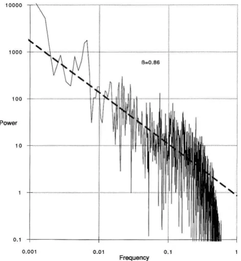
Fig. 3a. de Wijs Zinc concentration data from the Pulacayo mine,

Bolivia, withxthe horizontal distance in units of 2 m data (blue) simulation (pink with parametersα=1.8,C₁=0.03,H=0.090), both normalized to unity (the mean concentration is 15.6%).

we start with the assumption of a single regime and then only add new additional regimes when absolutely necessary.

Nevertheless, it is still important to directly verify the scal-ing on as many geophysically significant fields as possible; we discuss in particular the rock density, magnetic suscep-tibility, ore concentrations. Unfortunately, these generally require in situ measurements so that the corresponding hor-izontal fields are only known over sparse (possibly fractal (Lovejoy et al., 1986)) sets of sample locations. In prin-ciple this demands special multifractal interpolation tech-niques (Salvadori et al., 2001), but an operational method is still lacking. Cheng et al. (1994) has proposed a partial so-lution to this sparse measurements problem; the “Integrated spatial-spectrum Analysis” method. The first step is to use traditional Kriging methods to obtain a 2-D field on a uni-form grid. If the data are not too sparse (essentially they must be 2-D but with perhaps uniformly distributed “holes”), this may be adequate. The Kriging is followed this by spectral analysis. However instead of plotting the spectral density as a function of the modulus of the wavenumber (after

integrat-3/28/07 3

Fig. 3a, b

Fig. 3b. de Wijs spectrum: Red line is theory: 1–K(2)+2H with

K(2)=0.05 (trace moments),H=0.090 (first order structure func-tions), henceβh≈1.12.

ing in circles in Fourier space, see Eq. 2 above), the (Fourier space) log areas exceeding a log spectral density is plotted. If the process is isotropic in 2-D space, with spectral exponent β, then the result will be linear but with slope−1/(β−1) (the reciprocal because of the interchange of the ordinate and ab-scissa; the−1 because of the cumulation of all the values be-low a spectral density threshold). The method has the usual advantage that integrating smoothes the statistics, but has the added attraction of being insensitive to anisotropies (as long as the latter are scaling; it doesn’t involve integration over circles). Finally the method can be used to design new kinds of anisotropic filters useful for prospecting.

S. Lovejoy and D. Schertzer: Multifractals and the solid earth 471

3/28/07

4

-2 -1 0 1 2 3

-2,5 -2 -1,5 -1 -0,5 0 0,5

lo

g 10

E(k)

log₁₀k (cycles/m) 1

2 3 4 5 6 7 8

-3 -2 -1 0 1 2

lo

g

E(k)

log

10k (cycles/m)

Fig. 4a, b

Fig. 4a. Magnetic susceptibility spectra in the horizontal: Power

spectra for two sets of magnetic susceptibilities in the horizontal obtained by Pilkington and Todoeschuck (1993, 1995). The straight line shows the theoretical slopeβh=1.32.

3/28/07 4

-2 -1 0 1 2 3

-2,5 -2 -1,5 -1 -0,5 0 0,5

lo

gE(k)10

log₁₀k (cycles/m) 1

2 3 4 5 6 7 8

-3 -2 -1 0 1 2

lo

g 10

E(k)

log₁₀k (cycles/m)

Fig. 4a, b

Fig. 4b. Magnetic susceptibility power spectra from vertical

bore-hole logs in sedimentary (top) and igneous (bottom) rock from the same region as Fig. 4a (Pilkington and Todoeschuck, 1995). The straight line has the slope of 1.22. As discussed in Lovejoy et al. (2001) a values ofβh≈1.4 andβv≈1.2 gives a good explanation

for the observed surface gravity anomalies in the same (Canadian shield) region. The high wavenumber fall-off for the igneous series is probably due to slight oversampling.

spectrum is shown in Fig. 4a (Pilkington and Todoeschuck, 1995) which was obtained after Hankel transforming the ra-dial autocorrelation function from a sample of several thou-sand in situ susceptibility measurements. Due to the inad-equate sampling, the spectrum is not perfectly scaling, but coupled with a corresponding vertical (borehole) spectrum Fig. 4b, it turns out to be roughly what is required to explain magnetic surface anomaly spectra discussed in Sect. 2.4 be-low. Perhaps the most convincing of the horizontal in situ spectra are the 1-D “horizontal borehole” spectra of Leary

Fig. 5a. Horizontal borehole species: left to right gamma

emis-sion, rock density and seismic velocity absolute reference slopes =

βh=1.4, adapted from Leary (1997).

Fig. 5b. Vertical borehole analyses for the same quantities and

from the same region as Fig. 5a, the absolute reference slopes have

βv=1.2. Adapted from Leary (1997).

(1997) (Fig. 5a), for gamma emission, rock density and seis-mic velocity over the range of about 10 m to 1 km. Other ex-amples of horizontal analyses of in situ fields are hydraulic conductivity (see Fig. 6a), (Tchiguirinskaia, 2002) and car-bonate concentration (see Figs. 7a and 8a) (Tubman and Crane, 1995). These figures provide some of the rare ex-amples where both horizontal and vertical exponents from essentially the same regions have been analyzed; we could also mention the horizontal and vertical spectra in Shiomi et al. (1997). In Table 1, we summarize some of these results and we return to their implications for the stratification in Sect. 2.4.

2.3 Vertical scaling

We started out our survey of evidence for wide range scal-ing in the solid earth by considerscal-ing the horizontal direction; with the exception of the topography and remotely sensed radiances, surprisingly little is known about the horizontal scaling due to the difficulty in obtaining the necessary large quantities of in situ data. Although the geopotential fields (geomagnetism, geogravity) are relatively well measured (at least in certain regions) and do give us information about the horizontal structure, they also depend on the vertical struc-ture and for their interpretation require anisotropic scaling models of rock susceptibility and density respectively, see Sect. 2.4.

472 S. Lovejoy and D. Schertzer: Multifractals and the solid earth

3/28/07

7

Fig. 6a, b

βh=1.66, units are such that the lowest wavenumber is about 250 m,

highest about 10 m.

3/28/07

7

Fig. 6a, b

indicate βv=2.2 for hydraulic conductivity (bottom points) and

βv=1.5 for the logarithm conductivity data (top points),

how-ever the red line shows that the lower valueβv=1.3

(correspond-ing toHz=0.66/0.3=2.22) is a better fit for all except the highest

wavenumbers. Units are such that the lowest wavenumber is about 5 m, highest about 30 cm. Adapted from Tchiguirinskaia (2002).

parameters the vertical structure is better known than the hor-izontal due to the large number of borehole analyses. Ex-amples of scaling spectra from boreholes (gamma emission, rock density, magnetic susceptibility, sonic velocity, porosity, electrical resistivity) are Pilkington and Todoeschuck (1990),

3/28/07 8

Fig. 7 a,b

Fig. 7a. Horizontal power spectrum of the density of carbonate rock

well the last factors of 2 high frequency are a bit too smooth due to limitations of the data (no units given in the original). Reproduced from Tubman and Crane (1995),βh≈0.86.

3/28/07 8

Fig. 7 a,b

S. Lovejoy and D. Schertzer: Multifractals and the solid earth 473

3/28/07 9

Fig. 8

Fig. 8. Power law scaling of 3 well log and 3 small-scale resistivity

(FMS) power spectra over 5 decades of spatial frequency length (0.3 cycles/km to 60 cycles/km). Power law scaling exponentsβv

are 1.06 (P-wave sonic), 1.16 (S-wave sonic), 1.26 (density), 1.08 (FMS 1), 1.06 (FMS 2), 1.12 (FMS 3). Reproduced from Leary (2003b).

Todoeschuck et al. (1990), Todoeschuck and Jensen (1991), Bean and McCloskey (1993), Molz and Boman (1993); Molz and Liu (1997), Wu et al. (1994), Hollinger (1996), Leary (1997), Dolan et al. (1998), Leonardi and K¨umpel (1999), Tchiguirinskaia (2002), Leary (2003a), Marsan and Bean (1999, 2003), Dimri (2005). Other parameters such as ther-mal conductivities (Dimri and Vedanti, 2005) have also been shown to be scaling using other analysis techniques. Fig-ures 4b, 5b, 7b show some of the rare cases where both ver-tical and horizontal statistics can be compared allowing us to deduce the stratification exponentHz (Eq. 8). Figures 8, 9, 10 are shown because they are particularly striking exam-ples: Fig. 8 is a composite, but the spectra collectively cover a range of scales from centimeters to several kilometers, and Figs. 9, 10 show spectra of various parameters from the deep (KTB) borehole.

Two aspects of these analyses are particularly worth men-tioning. The first – widely recognized – is the proximity of many of theβ values to 1, hence the term “1/f noise”. This term originates in the ubiquitous noise in electrical circuits (due for example to contacts) with similar spectra. Indeed, Leary (1997) has argued that theβ’s of sonic velocities, rock densities, H2density (porosity), gamma activity and

resistiv-ity, porosity and permeability are all approximately unity (al-though with fluctuations of order 0.2–0.4) and he has argued that this could best be understood from a phase transition type mechanism such as percolation (for an introduction, see Stauffer, 1985, for applications to rock conductivity see Bahr, 2005, and references therein). The obvious problem with this as a general explanation is that in phase transitions, unless

3/28/07 10

Fig. 9

Fig. 9. Power spectrum of the KTB susceptibility (top) and density

(bottom) over the top 5596 m and 9098 m depths, respectively (2m resolution; wavenumberkin units of (2 m)−1). The reference slope hasβ=1.2 (authors’ analyses).

one happens to be exactly at the critical point there will only be scaling over a finite range of scales with a drastic break-down for larger scales. In addition, this critical scale diverges at the critical point so that one would expect to see scale breaks whose value depends sensitively on some physical pa-rameter such as porosity (indeed the possibility of such sen-sitive dependence of magma strength on porosity due to per-colation of bubbles has been suggested as a mechanism for volcanic eruptions (Gaonac’h et al., 2003, 20072). Although there are large fluctuations these are expected in scale invari-ant systems and the well logs all demonstrate wide range scaling with no obvious systematic or strong breaks. From the perspective of scale invariant dynamics (multifractal cas-cades, see below), the scaling can be roughly explained as follows: the scaling is due to the absence of a strong scale breaking mechanism and the value β close to one due to the fact that the observed processes are close to “conserved” multifractal processes which generically give spectra withβ a little below one (if not too intermittent). The empirical val-ues slightly above 1 are due to small degree of non scale by scale conservation; a parameterH >0, see below.

The second important point about the verticalβs (as men-tionned by Leary, 1997) is that the vertical and horizontal exponents are somewhat different. Indeed, the vertical expo-nents are systematically a bit closer to 1. As pointed out by Schertzer and Lovejoy (1985a) in the context of atmospheric stratification (and Lavall´ee et al., 1993) in the context of to-pography); if the horizontal and vertical scalings are differ-ent, then the corresponding structures will exhibit differential stratification; the key quantity is the ratioHz (Eq. 8) which we saw is the ratio of the horizontal to vertical structure func-tion/variogram exponents. From Figs. 4–8 we see that the stratification exponentHz≈1.7–2 for magnetic susceptibility

2_{Gaonac’h, H., Lovejoy, S., Nunes-Carrier, M., Schertzer, D.,}

474 _3/28/07 S. Lovejoy and D. Schertzer: Multifractals and the solid earth₁₁

Fig. 10

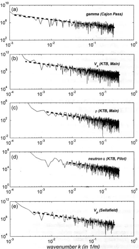
Fig. 10. Power spectra of five logs from various boreholes, from top

to bottom: (a) gamma log from the Cajon Pass borehole; (b) S-wave sonic log from the KTB main borehole, Germany; (c) resisitivity log from the KTB main borehole; (d) neutron porosity log from the KTB borehole; (e) P-wave sonic log from the Nirex 1 borehole at Sellafield UK. The dashed black lines give power law fitsk−βv _of

the spectrum decay, with spectral exponentβvequal to (a) 1.22,

(b) 0.98, (c) 1.31, (d) 1.37, (e) 1.4. All four boreholes probe the crystalline part of the upper crust. Reproduced from Marsan and Bean (2003).

(Lovejoy et al., 2001) andHz≈3 for rock density; (see Ta-ble 1). A valueHz>1 means that while the rock strata are very thin (highly flattened structures in vertical sections), that they nonetheless become progressively rounder at larger and larger scales (see Figs. 11, 14). In these examples, the sphero-scale is typically found to be quite large, thousands of kilometers. This is the opposite of the atmosphere where

3/28/07 12

Fig. 11

Fig. 11. Vertical cross-section of the magnetization scale function

assumingHz=2 and a spheroscale of (40 000 km)−1. The scale is

in kilometers and the aspect ratio is 1/4. Reproduced from Lovejoy et al. (2001).

the value Hz≈5/9 is found both theoretically and empiri-cally (see e.g. Schertzer and Lovejoy 1985a; Lilley et al., 2004) and the sphero scale is typically<1 m so that atmo-spheric structures become more and more stratified at larger and larger scales.

2.4 Combining Horizontal and vertical statistics: geopo-tential fields

Although over huge ranges of scale the processes which pro-duce variations in the lithospheric properties are undoubtedly highly nonlinear, some are sources for geopotential fields (notably geogravity, geomagetism) and are related to them by purely linear relations (Poisson’s equation, Maxwell’s equa-tions). Indeed, the relations are particularly convenient to deal with in Fourier space so that we can obtain very simple relations between the magnetic susceptibility spectrumPM, and the spectrum of the surface magnetic fieldPBor between the rock density and geogravity spectraPρ and Pg.

The example of magnetism and susceptibility has been studied in particular detail in Lovejoy et al. (2001) and Pec-knold et al. (2001). With various reasonable assumptions (that there is a scalar magnetic potential, that over the limited region of the study that the magnetic anomaly (B)and sus-ceptibility (M)have roughly constant directions so that only their magnitudes are variable), one obtains (see e.g. Blakely, 1995):

PB(K)= ∞ Z

kc

K2 K2_+k2

z

PM(K, kz) dkz (16)

The integration in the above is over all wavenumbers higher than the Curie wavenumber (kc≈2π/zcwherezcis the Curie depth at which all magnetization ceases due to high tempera-tures;zc≈30–80 km). In order to model the horizontal strat-ification, we takePM to be of the general anisotropic scaling form (Eq. 5). Using the susceptibility as a surrogate for the magnitude of the magnetizationM, from the data in Fig. 4a, b (see also Fig. 9), the valuesβM≈1.2,βhv≈1.4 can be used to determines≈4.4,Hz≈2 (Eq. 8) (Lovejoy et al., 2001).

S. Lovejoy and D. Schertzer: Multifractals and the solid earth_{3/28/07 13} 475

Fig. 12

Fig. 12. Power spectra of aeromagnetic anomaly fields from two

re-gional studies over the Canadian shield (triangles and circles). Su-perposed reference are lines with the theoretical high and low-wave number slopes,βBh=2,βBi=1 (see Eq. 17). The spectra have been

normalized so that the high wave number regions roughly coincide. Reproduced from Lovejoy et al. (2001).

spectrum; Fig. 12 shows that this is indeed the case on re-gionalBanomaly fields. The various relevant regimes are:

βBh=s−2;K > kc βBi =s−3;kc> K > Kic βBl = −3;K < Kic

(17)

whereKic=ks

kc

ks

1/Hz

is the horizontal wavenumber corre-sponding to the vertical Curie wavenumberkc, and theβB’s are the horizontal spectral exponents of the anomaly surface magnetic field andβBh, βBi,βBl are the high. intermedi-ate and low wavenumber spectral exponents. Since in the re-gion studied it was found thatks≈10−5_km−1_{,kc≈(30 km)}−1

andHz≈2, this implies Kic≈(1000 km)−1 so that the low wavenumber regime is masked by the contribution from the core, hence we only expect to see theβBh,βBi regimes with a break nearkc. Figure 13 shows that withs≈4.4, we can explain both: the same wide range but anisotropic scaling can explain the large scale earth magnetic anomalies up to several thousand kilometers (at larger scales it is dominated by the main dynamo component form the liquid core). Fig-ure 14 shows how stratified multifractal simulations (using the empirically determined universal multifractal parameters; see Sect. 5 below) can be used to simulate the magnetiza-tion, and Fig. 15 shows the correspondingBfields. See also Tennekoon et al. (2005) for scaling analyses of geomagnetic fields and Fedi (2003) for multifractal analysis of borehole susceptibilities.

Essentially the same type of relations hold between the vertical component of the surface gravity field (g) and the density of the rock (ρ):

Pg(K)=

Z _P

ρ(K, kz)

K2+k_z2 dkz (18)

3/28/07 14

Fig. 13

Fig. 13. Theoretical and experimental power spectra of surface

magnetic fields. The high wavenumber points are from data set 2 (circles) of Fig. 12, the high wavenumber points are from the global Magsat determined spherical harmonics (n=1 taken as (40 000 km)−1, from Langel and Estes, 1982). Reproduced from Lovejoy et al. (2001).

Maus and Dimri (1995, 1996) used this relation but with an isotropic (unstratified)Pρ in order to model high wavenum-ber surface gravity fields, Bourlon et al. (1998) proposed us-ing anisotropic scalus-ing. See also Bansal and Dimri (2005) which includes scaling analyses of the horizontal anisotropy of gravity anomalies. As in the case of the susceptibil-ity/magnetic anomaly relation, there are complications in the vertical so that there appear to be three regimes in the sur-face gravity field; essentially they are due to a) the mantle (low wavenumbers), b) the variable lithospheric thickness coupled with the strong mantle/lithosphere density gradient (intermediate range), c) the high wavenumber regime domi-nated by vertical and horizontal lithospheric heterogeneities (scales smaller than a hundred kilometers or so). While a de-tailed analysis of these contributions to the integral (Eq. 18) is in a forthcoming paper (Lovejoy et al., 2007a), the pa-rameterss=5.3,Hz=3 are roughly compatible with the high wavenumber regime and the horizontal and vertical density spectra published in Shiomi et al. (1997) and Leary (1997) (see Figs. 5, 9). Also, the mantle regime has been briefly dis-cussed in Lovejoy et al. (2005) and on the basis of an analysis of the equations of mantle convection, the parameterss=3, Hz=3 were proposed.

476 3/28/07 S. Lovejoy and D. Schertzer: Multifractals and the solid earth15

Fig. 14a,b,c

3/28/07 16

Fig. 14d

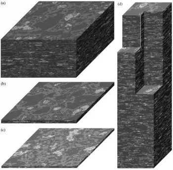
Fig. 14. (a) SimulatedMfield for horizontally isotropic crustal magnetization. The vertical anisotropy hasHz=1.7,s=4 and the universal

multifractal parametersH=0.2,C1=0.08,α=1.98. The sphero-scale was taken to be only≈2500 km; the simulation region is 32×32×16 km

with resolution 250 m. This is a reasonably realistic crustal section, although the sphero scale was taken to be a bit too small in order that strata may be easily visible. The direction ofMis assumed to be fixed in the z direction. (b) SimulatedMfor horizontally isotropic crustal magnetization; same parameters as (a). The simulation is 128×128×32 km; the resolution is 1 km and only the portion above the Curie depth of 10 km is shown. (c) SimulatedMfield for horizontally isotropic crustal magnetization; same parameters as (a). The simulation is 512×512×16 km; the resolution is 4 km. (d) SimulatedMfield the simulation is 4×4×16 km, resolution is 62.5 m. The cut-out shows the stratification and the presence of anomalies at all depths. Reproduced from Pecknold et al. (2001).

3 From fractal sets to multifractal fields, the limitations of classical geostatistics

3.1 Box counting, functional box counting

Using Fourier spectra, we have seen that many solid earth fields display wide range scaling in both horizontal and ver-tical directions. Spectra were first widely used to character-ize turbulence, and in the early 1970s in conjunction with the development of quasi-gaussian statistical closure mod-els, the theoretical or empirical determination of the spec-tral exponent became a key task. During the same period, Mandelbrot (1977) proposed using fractal geometry with its appealing promise of simplifying the description and model-ing of geoprocesses; in topography and geomorphology by

S. Lovejoy and D. Schertzer: Multifractals and the solid earth7/3/07 80 477

Fig. 15 a,b,c,d

Fig. 15. (a) The surfaceBfield from simulations shown in Fig. 14a. The Curie depth=16 km so that nearly the entire field shown is in the smooth, high wave number regimeβh=2. (b) The surfaceBfield corresponding to Fig. 14b. Since the entire region simulated is 128 km

across and the Curie depth is 10 km, the transition from high to intermediate wave number regime is in the middle of the range shown; the high wave number structures are noticeably smoother than the lower ones. (c) TheBfield corresponding to Fig. 14c; the entire simulation represents a region 512 km across, the Curie depth is 16 km so that most of the field shown with the exception of the very highest wave number structures is in the (rough) intermediate wave number regime withβi=1. (d) The same butBfor Fig. 14d, the entire field is in the

smooth high wave number regime. Reproduced from Pecknold et al. (2001).

However, by the early 1980s, the development of cascade models to study turbulent intermittency lead to the realization that in general an infinite number of dimensions were needed. The generic result of a cascade process (see Sect. 4 below) is that the cascade quantity at resolutionελhas the statistics:

hεq_λi =λK(q) (19)

whereK(q)is (convex) the moment scaling function andλis the ratio of the largest (outer) cascade scale and the scale of observation. The symbol “ε” is used for the turbulent (scale by scale) energy flux. Below, we discuss the link between these scaling exponents andξ(q) introduced earlier for the q-th order structure function and the spectral exponentβ.

Viewed from the point of multifractals, spectra are sec-ond order statistics so that the spectrum provide only a very partial statistical description. A more complete and direct description follows from the use of thresholds (T ) to con-vert fieldsε(x)into exceedance sets (xis a position vector),

and then the use of box-counting to systematically degrade the resolution of the sets, determining the fractal dimension using the formula:

NT(L)∝L−D(T ); PT(L)≈NT(L)/L−d ≈Lc(T );

c(T )=d−D(T ) (20)

478 S. Lovejoy and D. Schertzer: Multifractals and the solid earth

3/28/07 18

Fig. 16a

Fig. 16a. Functional box-counting on French topography data at

1 km resolution. For each threshold, the scaling is quite accurate, but as the threshold increases, the slope systematically decreases so that the topography is apparently not monofractal. The line with slope−2 is shown since this is the theoretical assumption of classi-cal geostatistics. Adapted from Lovejoy and Schertzer (1990).

of multifractals). Indeed wheneverD(T )<d, the stochastic codimension functionc(T )defined by Eq. (20) is equal to the geometric codimension functiond−D(T ); however, in generalc(T )will be unbounded. For the corresponding ex-treme events, if one usesD(T )=d−c(T ), one would obtain the geometrically impossible valuesD(T )<0. By using the statistical codimension we thus avoid the paradox negative or “latent” dimensions (Mandelbrot, 1983).

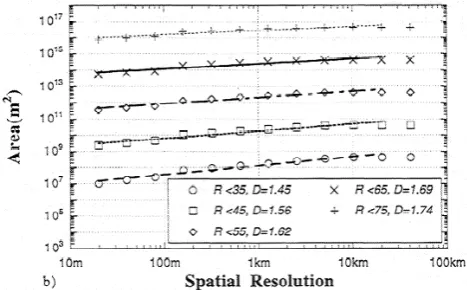
When this “functional” box-counting (Lovejoy et al., 1987) was applied to the topography (Fig. 16a) it was found that the scaling was excellent: the power law Eq. (20) was accurately obeyed for allT,L. However – as expected for a multifractal –D(T )systematically decreases with threshold, it is not constant as assumed in the monofractal models. In-deed, from the point of view of multifractals, it would have been a miracle if for each thresholdT, each (different) set had exactly the same fractal dimension. Figure 16b shows the results of functional box-counting on reflected visible radi-ances from lava flows, showing both the excellent wide range scaling of the flows and also the systematic decrease ofD(T ) withT. In this figure we directly see a consequence: the ar-eas of lava flows exceeding a threshold depend in a power law way on the resolution:AT(L)≈L2L−D(T ), we return to this important point below.

If the topography could be adequately modeled as a geo-metrical fractal set, then many different techniques (includ-ing spectral analysis) could be used to estimate its unique di-mensionD. However, due to the multifractality evidenced in the functional box-counting (Fig. 16), on the contrary, when

3/28/07 19

Fig. 16b:

Fig. 16b. A log-log plot of the areas (AT(L)≈L2L−D(T ))of SPOT

satellite radiances of Mauna Lao volcano (visible, 20 m resolution) exceeding a radiance thresholdT=R(in digital counts), with corre-sponding fractal dimensions indicated. Each line has been offset by 2 orders of magnitude for clarity. Reproduced from Laferri`ere and Gaonac’h (1999).

different analysis techniques were applied to different data sets commonly gave different values ofD. In particular the empirical topography spectral exponentβ≈2 (Fig. 1) would implyD=2.5 for monofractal surfaces (1.5 for monofractal vertical sections) whereas the (rare) direct estimates (Good-child, 1980; Aviles et al., 1987; Okubo et al., 1987; Turcotte, 1989) commonly gave a diversity of values (see the reviews Klinkenberg and Goodchild, 1992; Maliverno, 1995).

The use of simplistic monofractal ideas had consequences beyond a failure to reach consensus on a supposedly “unique” fractal dimension of the topography. Due to their random singularities, multifractals have such strong vari-ability that they violate many conventional geostatistical as-sumptions so that normal multifractal variability can easily be misinterpreted in terms of spurious scale breaks, spurious nonstationarity etc. The loss of interest in scaling was en-couraged by the extensive use of (low variability) fractional Brownian motion (fBm) models of topography. As argued in Gagnon et al. (2006), the topography in fact has excellent multiscaling (multifractal) properties (see Figs. 1, 16a, 18) – but an infinite hierarchy of fractal dimensions; this requires new analysis techniques.

S. Lovejoy and D. Schertzer: Multifractals and the solid earth_{3/28/07 20} 479

Fig. 17

Fig. 17. Lava flows from mount Etna 1900–1974 taken from a geological map at 43 m resolution. The resolution is then successively

degraded by factors of 2 using box counting. Reproduced from Gaonac’h et al. (1992).

adequate theoretical framework for scaling has thus led the baby to be thrown out with the bathwater.

3.2 Consequences for classical geostatistics

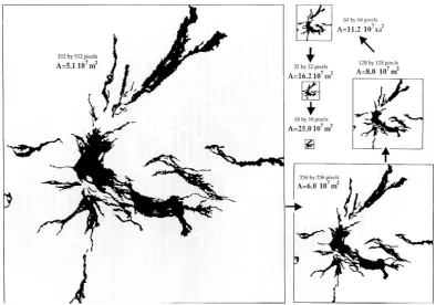
It is worth mentioning that the functional box-counting re-sults (Fig. 16) have direct and important consequences for classical geostatistics (e.g. Matheron, 1970) which assume (explicitly or implicitly) that geomeasures such as the areas of the topography exceeding a threshold are regular with re-spect to Lebesgue measures. If this assumption were true, then the areas above a given threshold T would be well-defined independently of the resolutionL, i.e. the expression L2NT(L)would be independent ofLfor smallL; however sinceD(T )<2 we see that generally it vanishes asL→0. Ul-timately at small scales – probably millimeters or less – the scaling will break down yielding a finite limit ofL2NT(L). However the area estimated L2NT(L) will depend on the very small scale details; at any larger resolutions the result will be subjective depending on the observing resolutionL. While Fig. 16b shows this directly on various sets defined by radiance thresholds on volcanoes, Fig. 17 shows the same ef-fect visually, using step by step degradation of the resolution of lava flow maps determined by geological mapping tech-niques. The usual box-counting method is used to succes-sively degrade the resolution of the flows. As the resolution improves by a factor of 512/16=32, we see (moving in the

direction opposite the arrows) more and more fine details. Over this scale factor, the area decreases by a factor of about 5 corresponding to a fractal dimension of the areas of about 1.58; the fractal dimension of the perimeter set is 1.42 so that it is a little bit sparser.

If we express the field values as powers of the resolution with random exponents γ, i.e. if we writeT∝λγ then we obtain:

Pr(ελ> T )=Pr(ελ> λγ)∝λ−c(γ ) (21) where “Pr” indicates “probability”. For cascade processes, we derive this result directly in Sect. 4.3. Since the moments (Eq. 19) are integrals over the probability density (dPr),c(γ ) determinesK(q); we discuss this link in Sect. 4.7.

480 3/28/07 21 S. Lovejoy and D. Schertzer: Multifractals and the solid earth

Fig. 18

Fig. 18. Log-log plot of the normalized moments versus the scale

ratioλ=Louter/l(withLouter=20 000 km) for the three DEM’s

(cir-cles correspond to ETOPO5, X’s to U.S. (GETOPO30), and squares (Lower Saxony). The solid lines are there to distinguish between each value ofq(from top to bottom,q=2.18, 1.77, 1.44, 1.17, 0.04, 0.12, 0.51) The trace moments of the Lower Saxony DEM with rees forq=1.77 andq=2.18 are on the graph (indicated by arrows). The theoretical lines are computed with the globalK(q)function dis-cussed with universal multifractal parametersα=1.79,C1=0.12. At

scales<40 m, in this Lower Saxony data set, the effect of trees be-comes important, apparent increasing the variability at the smallest scales. Reproduced from Gagnon et al. (2006).

determine the moment scaling exponentK(q). To do this, we take for the multifractal fieldε3the absolute gradients of the topography at the finest resolution of the data set3=L/l whereLis the external scale (taken as 20 000 km here) andl is the pixel scale (see Sect. 4.10 for more discussion of this). The result of degrading the high resolutionε3to intermedi-ate scale ratiosλis shown in Fig. 18 (using the same data sets as in Fig. 1). We can see that the multiscaling holds very well over a factor of more than 105in scale. Indeed, Gagnon et al. (2006) estimates that the “reduced moments”<εq_λ>1/q for allq≤2 can be reproduced to within±45% using just a 2 parameter “universal multifractal” fit to theK(q)function (Eq. 45; see Sect. 4.6). Other relevant examples of multifrac-tal analysis are soil moisture (Dubayah et al., 1997), LAND-SAT TM channels (Cheng, 1999), sonic velocities (Marsan and Bean, 1999) and neutron porosity (Marsan and Bean, 2003); Figs. 25a, b (the latter two in the KTB borehole). In Sect. 4.10 we perform various multifractal analyses on the de Wijs (1951) Zn concentration series.

3.4 Multifractality and spurious breaks

In spite of the systematic finding of scaling or near scal-ing statistics, many geophysicists instinctively reject all wide range scaling; they consider a priori that the scaling is bro-ken. However conclusions about broken scaling are

fre-quently unwarranted. Perhaps the most important source of misinterpretation is the fact that scale invariance is a statisti-cal symmetry which is almost surely broken on every single realization, hence it is important to have a large data base (i.e. large range of scales, many realizations) to average fluctua-tions and to approximate the theoretically predicted ensem-ble average scaling. In fact, due to the singularities of all or-ders (see the previous section) the variability of multifractals is much greater than that of classical stochastic processes; for example, rare (extreme) singularities are produced by the process yet they are almost surely absent on any given real-ization. This means that multifractal processes generally do not have the property of “ergodicity”. What may be noth-ing more than normal multifractal statistical variability can thus easily be interpreted as breaks in the scaling. A second reason for unwarranted rejections of scaling is the assump-tion that the scaling is isotropic. If the scaling is anisotropic, there may be breaks in the scaling on 1-D subspaces (e.g. transects) but not for the full process in the higher dimen-sional space in which they evolve. A third reason discussed in more detail in Gagnon et al. (2006) is that there can be systematic biases due to the use of conditional statistics such as studying transects that just happen to pass through special features (such as high mountains).

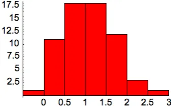
There are also nonclassical statistical effects which can lead to yet other misinterpretations of the data. One of these is a consequence of the fact that the strong singularities in multifractals leads to apparent nonstationarities: e.g. to quite different morphologies which can often be found in close proximity. This is often interpreted in terms of nonstationar-ities/spatial inhomogeneities – different processes at work in different regions or at the very least, variations in the param-eters of a single basic model. However, with multifractals such interpretations would be unwarranted: the basic multi-fractal processes are statistically stationary/homogeneous in the strict sense that over the region over which they are de-fined (which is necessarily finite), the ensemble multifractal statistical properties are independent of the (space/time) lo-cation (and this – contrary to certain affirmations in the liter-ature – for any spectral slopeβ). Rather than discussing this at an abstract level, let us see what happens when we analyse a self-similar 1024×1024 multifractal simulation (Fig. 19a). In the simulation, consider the “regional” variability in the spectral exponentβ by dividing it into 8×8 squares, each with 128×128 pixels. Figure 19b shows the histogram of the 64 regression estimates of the spectra compensated by the theoretical behaviour i.e.E(k)/(k−βtheory_)withβ

theory=2.17.

As expected, the mean is close to zero but we see a large scat-ter implying that there are some individual regions havingβ as low as 1.2, some as high as 2.7; the standard deviation is

S. Lovejoy and D. Schertzer: Multifractals and the solid earth 481

3/28/07 22

Fig. 19a

Fig. 19a. A self-similar multifractal (with some trivial anisotropy)

simulated on a 10–24×1024 poihnt grid with observed universal multifractal parameters (H=0.7,C₁=0.12,α=1.9); the spectral exp-nent isβ=1+2H−K(2)=2.17. Adapted from Gagnon et al. (2006).

Fig. 19c, we can also see the large variations in the log pref-actors (log10E1;E(k)=E1k−β). IfE1is interpreted in terms

of roughness, the roughest of the 64 regions has about 103 times the variance of the smoothest. While it would obvi-ously be tempting to give different interpretations to the pa-rameters in each region, this would be a mistake. The phys-ical interpretation of such a model is that the roughest and the smoothest are associated with huge variations in the cor-responding erosional, orographic and other processes; this would follow if these processes are also scaling and would have correlated variations.

4 Cascades and multifractals

4.1 Ore distributions, the de Wijs binomial cascade, the lognormal versus Pareto debate

We have seen that there is much evidence for the wide range scaling of various geophysical fields in both the horizontal and vertical directions from sub metric to the largest scales probed by the deepest boreholes (several kilometers) in the vertical and from sub metric to planetary scales in the hori-zontal. So far, we have not made a serious attempt to explain these results except to comment that since scale invariance is a symmetry principle, the nonlinear dynamics which are re-sponsible for the wide range heterogeneity must repeat scale after scale in a cascade like manner. We now turn to the generic cascade process.

7/3/07 86

Fig. 19b: (left): Fig. 19c(right).

Fig. 19b. After dividing Fig. 19a into 64 128×128 squares, we calculated the isotropic spectrum in each, and fit the slope to the lowest factor 16 in scale (we remove the highest factor 4 due to numerical artifacts at the highest wavenumbers). The resulting1β

is given in the left; it is twice the1H, showing that H can vary by 0.5 over a single region. From Gagnon et al. (2006).7/3/07 86

Fig. 19b: (left): Fig. 19c(right). Fig. 19c. A histogram of the log

10E1(E1is the spectral prefactor: E(k)=E1k−β)showing variation of 1000 from the smoothest to

roughest subregion. From Gagnon et al. (2006).

482 3/28/07 S. Lovejoy and D. Schertzer: Multifractals and the solid earth24

Fig. 20

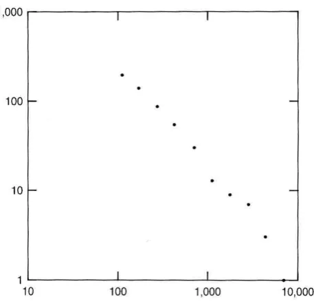
Fig. 20. Ore valuations of a South African Mine; “cumulated

Pare-tian graphs” i.e. doubly logarithmic plots of the numbers of valua-tions exceeding a given valuation. The distribution is nearly hyper-bolic (linear on this plot) with exponentqDnear one (Krige, 1960)

(reprinted in Mandelbrot, 1995).

De Wijs was interested in the concentration of ores and was debating the form of their probability distributions. Along with Lasky (1950), he defended the idea that the prob-abilities were log-normal, criticizing (Van Tongeren, 1950) who on the contrary defended algebraic (power law) distri-butions. In order to help prove his point he proposed a sim-ple cascade model which he called the “binomial” model. At the time, some of the proponents of log-normality even went so far as to propose it as a the first law of geochemistry (Ahrens, 1953). The debate about lognormality versus power law (often called “Pareto” in this context) continued through the 1960s to the 1980s, with notably Matheron (1962) siding with the lognormal camp; see also Cargill et al. (1981) and Agterberg (2007). In the 1980s, this binomial model was rediscovered by and applied in geology to the distribution of fossils (Plotnick and Prestegaard, 1995), while Turcotte (1986) made a drastic modification to the cascades so as to generate a Pareto distribution (see Sect. 4.8 below). In the turbulence literature the binomial model became known as the “pmodel” (Meneveau and Sreenivasan, 1987); we shall see below that it is actually a microcanonical restriction on the “αmodel” (Schertzer and Lovejoy, 1985a).

To put the debate in perspective, we show Fig. 20 which is an example of the distribution of ore grades indicating that empirically, they can be far from log-normal (Krige, 1960; reprinted in Mandelbrot, 1995); see Fig. 3 and below for a re-examination of the de Wijs data). Note that Cheng et al. (1994), and Cheng (2000a) proposed a variant of the method of plotting in Fig. 20 called the “Concentration-area

fractal method” involving plotting the logs of the areas of metal bearing ores exceeding various concentration thresh-olds, the latter also plotted on a log scale.

4.2 The binomial/p model and theαmodel

In order to demonstrate how a roughly log-normal distribu-tion of ores might arise, de Wisj considered a 1-D secdistribu-tion which he successively divided into two equal halves; he then reasoned that various processes might concentrate the mate-rial in the left segment by a factor (1+d)reducing the con-centration on the right segment by the factor (1−d) where 0≤d≤1 is the “dispersion index”; empirically for many ore concentration series, de Wijs found d≈0.2 (typical of iron and zinc deposits), although for precious metals, values as high as 0.45 were obtained (see also Agterberg, 2007, for more examples). He then considered the effect of repeating this multiplicative construction to smaller and smaller scales (but without considering the nontrivial mathematical limit).

In order to understand this, let’s change the notation and generalize this slightly. Denote byλthe division ratio, and the multiplicative factors byµεi(in analogy with the symbol “1x” for an additive increment), where “i” indexes the fac-tors (left or right which can be chosen randomly); andDthe dimension of the space. de Wijs’s model thus corresponds toλ=2,D=1 and the valuesµε+=(1+d),µε−=(1−d)were always chosen together (left or right) so that they satisfy:

1 λD

λD

X

i=1

µεi =1 (22)

whereµεi=µε+orµε−. The sum ensures that the increase (decrease) in ore in the left half is exactly compensated by a decrease (increase) in the right half. Ifλ>2 and/or ifD>1 then there can be several states but at each step, each “parent” and “daughter” structures satisfy the restriction Eq. (22). In analogy with statistical mechanics, this strict scale by scale conservation is called “microcanonical” (Mandelbrot, 1974). To obtain the more general “canonical” cascade, it suffices to replace the microcanonical conservation by:

hµεi =1 (23)

where “<.>” indicates ensemble averaging; in the canoni-cal cascade the left and right hand factors are thus chosen independently of each other. The resulting two state model (in any dimensionD)was called the “αmodel” (Schertzer and Lovejoy, 1985a) (see Fig. 21) in order to distinguish it from the pure fractal “βmodel” (Frisch et al., 1978). To un-derstand the statistics of these binomial processes, write the probabilities of the model states as follows:

Pr(µε=_λγ+_)=λ−c_{(>1⇒ increase)}

S. Lovejoy and D. Schertzer: Multifractals and the solid earth 483

3/28/07 25

1

x

0

1

x

1

! _!

"

#₊

$ #

"

Simple Cascade Models ( and -model):% & ( -instability)%

Fig. 21a

Fig. 21a. Illustration of the α model: here εn=µε·εn−1.

The weak sub-eddies have an associated probability Pr(µε=_λγ−_)=1−λ−c_(γ

−<0) whereas the strong sub-eddies have Pr(µε=_λγ+_)=λ−c_(γ+>0).

3/28/07 26

+

+

+

+

+

+ +

_

_

_

_

_

_

_

+

Fig. 21b. Schema of tree of singularities for a one-dimensionalα

model the “+” indicates a choice ofγ+, the “–”,γ− , with proba-bilities as above. The microcanonical “de Wisj” (or “binomial” or “p” model) would have “+” and “–” always occurring in pairs so that at each scale and each location, the total ore amount is rigidly conserved.

de Wijs model is recovered with the parametersλ=2, c=1, γ+=logµε+/logλ=logλ(1+d), γ−=logµε−/logλ=logλ(1−d) and with the additional condition that the only randomness is to choice of which of the two is left or right.

In theαmodel, the canonical conservation condition im-plies:

λγ+_·λ−c_+λγ−_·(1−λ−c_{)=1 (25)} because of this constraint out ofc,γ+andγ−, there are really only two free parameters, this is valid for any λ, D. For the microcanonical model, the conservation condition on the contrary depends not only onλ, but also onD. A purely “all or nothing” process called the “β-model” (Frisch et al., 1978) is obtained withγ−=−∞; this is the monofractal limit; the nonzero region is a fractal set with codimensionc.

Wheneverγ₋>−∞and the process is iterated, the pure orders of singularity γ− andγ+ lead to the appearance of mixed orders of singularity, (the “αmodel”). Mixed singu-larities of different ordersγ (γ−≤γ≤γ+)are built up step by

3/28/07 27

Fig. 21c

Fig. 21c. Theαmodel in 2-D showing both the bare (left) and dressed cascades (right). Reproduced from Wilson (1991).

step through a complex succession ofγ− andγ+, as illus-trated in Fig. 21b. Figure 21c shows a 2-D example of theα model which we will study in more detail in the next section. In other words, leaving the simplistic alternative dead or alive (“β model”) for the alternative weak or strong (”αmodel”) leads to the appearance of a full hierarchy of levels of sur-vival, hence the possibility of a hierarchy of dimensions. 4.3 Renormalizing discrete cascades

What is the behavior as the number of cascade steps,n→∞? Consider two steps of the process, the various probabilities and random factors are:

Pr(µε=_λ2γ+_)=λ−2c _{(two boosts)}

Pr(µε=_λγ++γ−_)=2λ−c_(1−λ−c_{)(one boost and one decrease)} Pr(µε=_λ2γ−_)=(1−λ−c₎2 _{(two decreases)}

484 S. Lovejoy and D. Schertzer: Multifractals and the solid earth This process has the same probability and amplification

fac-tors as the three-stateαmodel with a new scale ratio ofλ2, i.e.,

Pr(µε=_(λ2)γ+)=_(λ2)−c Pr(µε=_(λ2)(γ++γ−)/2

)=2(λ2)−c/2−2(λ2)−c Pr(µε=_(λ2)γ+)=1−2(λ2)−c/2+_(λ2)−c

(27)

Iterating this procedure, aftern=n++n−steps we find: γ_n+_,n− =n

+_γ ++n−γ− n+_+n− , n

+_{=1, ..., n} Pr(µε=_λγn+,n−₎=

n n+

λ−c n+(1−_λ−c)n

− (28)

where

n k

is the number of combinations ofnobjects taken kat a time. This implies that we may write:

Pr(ε_λn ≥(λn)γi)=₆

j

p_ij(λn₎−cij ₍₂₉₎

The pij’s are the “submultiplicities” (the prefactors in the above),cij are the corresponding exponents (“subcodimen-sions”) and λn is the total ratio of scales from the outer scale to the smallest scale. Notice that the requirement that

hµεi=1 implies that some of the λγi _{are greater than one}

(boosts) and some are less than one (decreases), that is some γi>0 and someγi<0. Note also that theα-model will have bounded singularities:

γ−≤γi ≤γ+ (30)

(i.e., the maximum attainable singularity γmax is equal to

γ+). The final step in “renormalizing” the cascade is to re-place the above n-step (ratioλ), 2-state cascade by a single λnstep cascade withn+1 states. Note that we are not saying that there is absolutely no difference between the n-state α-model with ratioλand the corresponding (n+1)-state model withλ0=λn; however their properties will be identical for integral powers ofλ0. Finally, doing this and making the re-placementλn→λ, and the limitλ→∞, one of the terms in the sum will dominate (that with the smallestcij). Hence defining

ci =mincij =c(γi) (31) yields forλ→∞:

Pr(ελ≥λγi)=pi·λ−ci (32)

whereci is the codimension andpi is the multiplicity. If we now drop the subscripts “i” (this allows for the possibility of a continuum of states, e.g., the original process being de-fined by a uniform or other continuous distribution) then we obtain:

Pr(ελ≥_λγi_)∼λ−c(γ )_{·p(γ );} dc

dγ >0 (33)

This is a basic multifractal relation for cascades. We now simplify this using the “∼” sign which absorbs the multi-plicative (p(γ ))as well as taking into account the mic number of terms in the sum (which can lead to logarith-mic prefactors corresponding to “sub-codimensions”). With this understanding about the equality sign, we may write

Pr(ελ≥λγ)∼λ−c(γ ) (34)

Each value ofελcorresponds to a singularity of orderγ and codimensionc(γ ). Note that strictly speaking the expression “singularity” applies toγ >0 (forλ→∞), whenγ <0 it is a “regularity”.

In the geophysics literature, there has also been a variant on the microcanonical cascade called the “bounded cascade” (Cahalan, 1994) in which the cascade is progressively killed as the cascade proceeds by multiplying each 1–µεi byrn where 0<r<1 andnis the number of cascade steps from the beginning of the cascade. In this way, the dispersion coef-ficientsd algebraically decreases: dn+1=rdn so that rapidly all theµεi≈1. This has the drastic effect of essentially de-stroying the multiplicative nature of the cascade at the small scales, effectively turning it into an additive process (Love-joy and Schertzer, 2006). In the small scale limit we ob-tain essentially a truncated Brownian motion with only triv-ial multifractality. Another variant on the basic microcanon-ical model has been proposed by Cheng (2005). In this 2-D model, there are 4 different weightsµεwhich are chosen de-terministically always in the same 2X2 pattern. The resulting cascade is generally anisotropic. Although Cheng notes that no scale by scale conservation property generally holds on 1-D sections (this presumably leads to nontrivial problems of convergence in the small scale limit), this model is proposed for anisotropic multifractal fields.

4.4 Unlocalized versus localized singularities

Note that while the above form of the probability distribu-tions/histogram Eq. (34) is valid at every step of the cascade process (every finiteλ), this in no way implies that there is convergence ofγ at a given mathematical pointx. Indeed for canonical cascades, in general we have lim

S. Lovejoy and D. Schertzer: Multifractals and the solid earth 485

(a)

7/3/07

92

Fig 22 a,b,c,d

(b)

7/3/07

92

Fig 22 a,b,c,d

(c)

7/3/07

92

Fig 22 a,b,c,d

(d)

7/3/07 92

Fig 22 a,b,c,d

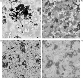
Fig. 22. The anatomy of a singularity. (a) Upper left is full (continuous in scale) simulation 216long with universal multifractal parameters

α=1.8,C1=0.05 (close to de Wijs data values for Zn ore). Black is the full resolution data, pink is low resolution, degraded by a factor of

64. (b) The upper right shows a zoom (factor 16) into the section with the maximum value, (c) the lower left is a zoom by a further factor 20 near the maximum; the arrows show the position of the high resolution maximum as well as the centre of the low resolution maximum.

(d) The lower right is the same but on log-log plot using distance from the maximum. The pink shows the approach to the maximum

low resolution singularity on the low resolution series with the green being the rms fit giving the estimate 0.63 (the absolute slope) for the maximum singularity, showing it’s