www.atmos-meas-tech.net/9/3687/2016/ doi:10.5194/amt-9-3687-2016
© Author(s) 2016. CC Attribution 3.0 License.
A new set-up for simultaneous high-precision measurements of CO
2
,
δ
13
C-CO
2
and
δ
18
O-CO
2
on small ice core samples
Theo Manuel Jenk1,a, Mauro Rubino2,b, David Etheridge2, Viorela Gabriela Ciobanu1, and Thomas Blunier1 1Centre for Ice and Climate, Niels Bohr Institute, University of Copenhagen, Copenhagen, Denmark
2CSIRO Oceans and Atmosphere, Aspendale, Victoria, Australia
anow at: Paul Scherrer Institute, Laboratory of Environmental Chemistry, Villigen PSI, Switzerland bnow at: Seconda Università degli Studi di Napoli, Caserta, Italy
Correspondence to:Theo Manuel Jenk ([email protected])
Received: 13 November 2015 – Published in Atmos. Meas. Tech. Discuss.: 1 February 2016 Revised: 16 May 2016 – Accepted: 21 June 2016 – Published: 10 August 2016
Abstract.Palaeoatmospheric records of carbon dioxide and its stable carbon isotope composition (δ13C) obtained from polar ice cores provide important constraints on the natural variability of the carbon cycle. However, the measurements are both analytically challenging and time-consuming; thus only data exist from a limited number of sampling sites and time periods. Additional analytical resources with high ana-lytical precision and throughput are thus desirable to extend the existing datasets. Moreover, consistent measurements de-rived by independent laboratories and a variety of analytical systems help to further increase confidence in the global CO2
palaeo-reconstructions. Here, we describe our new set-up for simultaneous measurements of atmospheric CO2mixing
ra-tios and atmospheric δ13C and δ18O-CO2 in air extracted
from ice core samples. The centrepiece of the system is a newly designed needle cracker for the mechanical release of air entrapped in ice core samples of 8–13 g operated at
−45◦C. The small sample size allows for high resolution and replicate sampling schemes. In our method, CO2is
cryo-genically and chromatographically separated from the bulk air and its isotopic composition subsequently determined by continuous flow isotope ratio mass spectrometry (IRMS). In combination with thermal conductivity measurement of the bulk air, the CO2 mixing ratio is calculated. The
ana-lytical precision determined from standard air sample mea-surements over ice is ±1.9 ppm for CO2 and±0.09 ‰ for δ13C. In a laboratory intercomparison study with CSIRO (Aspendale, Australia), good agreement between CO2 and δ13C results is found for Law Dome ice core samples. Repli-cate analysis of these samples resulted in a pooled standard
deviation of 2.0 ppm for CO2 and 0.11 ‰ forδ13C. These
numbers are good, though they are rather conservative esti-mates of the overall analytical precision achieved for single ice sample measurements. Facilitated by the small sample re-quirement, replicate measurements are feasible, allowing the method precision to be improved potentially. Further, new analytical approaches are introduced for the accurate correc-tion of the procedural blank and for a consistent deteccorrec-tion of measurement outliers, which is based onδ18O-CO2and the
exchange of oxygen between CO2 and the surrounding ice
(H2O).
1 Introduction
Polar ice cores are unique in providing direct information of the past atmospheric composition. Analysis of entrapped air allows the evolution of the atmospheric composition over the last 800 000 years to be reconstructed (e.g. Lüthi et al., 2008 and references therein; Bereiter et al., 2015). Knowledge of past natural CO2 variations – only several ppm during the
Holocene and up to about 100 ppm over glacial/interglacial changes – is crucial to improve predictions of future climate under continued anthropogenic CO2forcing. Changes in the
global carbon cycle fluxes are imprinted in the stable carbon isotope signal of atmospheric CO2(δ13C, e.g. Köhler et al.,
1999; Smith et al., 1999; Elsig et al., 2009; Lourantou et al., 2010a, b; Schmitt et al., 2012; Rubino et al., 2013; Schneider et al., 2013; Bauska et al., 2015).
Since the pioneer CO2measurements in the 1980s (Berner
et al., 1980; Delmas et al., 1980; Neftel et al., 1982; Pear-man et al., 1986), extraction and measurement techniques have been continuously developed and improved to increase the analytical precision. The initial step of extracting air en-trapped in ice is crucial. While extraction of gas by melt-ing the ice is successfully applied for trace gases like CH4,
CO2measurements are generally not reliable in the presence
of liquid water (Kawamura et al., 2003). Measurement arte-facts arise due to the high solubility of CO2 and chemical
reactions of carbonate species in water (Anklin et al., 1995; Zhang et al., 1995; Kawamura et al., 2003). Further chal-lenges arise from adsorption, desorption and contamination effects at surfaces, particularly in connection with mechan-ical friction between system components (e.g. Zumbrunn et al., 1982), from system leakage, outgassing materials and in-troduction of contaminants (e.g. drilling fluid). In order to avoid the liquid phase of water, the air must either be ex-tracted in a cooled vacuum chamber by dry mechanical tech-niques (e.g. Bauska et al., 2014) or by sublimation of the ice matrix (e.g. Schmitt et al., 2011).
When the enclosed air is available in the form of bubbles, the gas extraction efficiency for mechanical systems varies between 60 % and∼90 %. However, in deeper strata where the gas is present in air hydrates (e.g. Uchida et al., 1994) – also called clathrates – extraction efficiencies usually de-crease by 10–20 %. For the transition zone, where air bub-bles and clathrates coexist, it has been found that CO2is
en-riched in clathrates and depleted in air bubbles. In this zone, measurements of CO2mixing ratios can thus be severely
bi-ased as they depend on the gas extraction efficiency (Ikeda et al., 1999; Sowers and Jubenville, 2000; Ahn et al., 2009; Schaefer et al., 2011; Bereiter et al., 2014). At the cost of a slow extraction process which limits sample throughput, this problem can be avoided by sublimation of the ice matrix, re-sulting in close to 100 % extraction efficiency (Güllük et al., 1998; Schmitt et al., 2011). Anyhow, while measurements of CO2 mixing ratios by mechanical extraction systems are
affected in the transition zone from bubble to clathrate ice, only a decrease in precision but no systematic effect could be observed forδ13C analysis of CO2(Schaefer et al., 2011
and references therein). In addition, for pure bubbly ice, the extraction efficiency is not a concern for CO2measurements
and no difference has been observed compared to results de-rived by sublimation systems.
A variety of mechanical extraction systems are in use. In a needle cracker (NC), the ice is crushed to small pieces and air is released from the thereby opened bubbles (Zumbrunn et al., 1982). The system described by Bereiter et al. (2013) pul-verizes ice samples by continuously shaving off thin layers of the sample surface by a centrifugal ice microtome (CIM). Al-ternatively, ice samples are ground in a ball mill when both
the ice sample and stainless steel balls inside a small con-tainer are shaken (Barnola et al., 1995; Lourantou, 2009), or grated into small chips by shaking the ice in a vessel contain-ing a perforated inner cylinder (“cheese grater”, Etheridge et al., 1996).
Only a few laboratories have the ability to do ice core anal-ysis of both CO2concentrations and its stable isotopic
com-position. In the following, the published and recently oper-ated analytical systems allowing measurements of both pa-rameters on a single ice sample are summarized (see Table 1 for detailed system characteristics). All systems use isotopic ratio mass spectrometry (IRMS) to detect the different mass ratios between the stable CO2isotopologues (m/z44, 45 and
46).
The Laboratory of Climate and Environmental Physics (KUP, Bern, Switzerland) operates two such systems. For the mechanical extraction system (NC) the released air is first expanded over a water trap into a small volume where the gas pressure is measured for evaluation of the CO2 mixing
ratio in combination with the IRMS signal. Using helium as a carrier gas, the gas sample is then flushed into a pre-concentration system (PreCon) to separate the main com-ponents of air. In order to avoid isobaric interference, CO2
is separated from N2O and organic compounds (e.g. from
drilling fluids) by gas chromatography (GC) before being in-jected into the IRMS via an open-split interface (Elsig et al., 2009). In the sublimation system, sublimated water is quan-titatively removed before the liberated air is cryogenically collected. Then, the basic principle is similar to the system described before but extraction and GC–IRMS are decoupled (Schmitt et al., 2011). KUP additionally operates one system (CIM) solely dedicated to the analysis of the CO2 mixing
ratio (Bereiter et al., 2013), which replaces their initial NC system described by Zumbrunn et al. (1982) and modified by Lüthi (2009).
The Laboratoire de Glaciologie et Géophysique de l’ En-vironnement (LGGE, Grenoble, France) uses a ball mill for mechanical extraction before the air is directly released to the inlet system of a coupled GC–IRMS for CO2 mixing
ratio and CO2stable isotope analysis (Barnola et al., 1995;
Lourantou, 2009).
The ice core and quaternary geochemistry lab at Oregon State University (OSU, USA) also uses a mechanical extrac-tion system (cheese grater). A small aliquot of the extracted sample gas is isolated from the grater and finally trapped at
−260◦C after water is removed at−100◦C. The CO2
mix-ing ratio is then determined by GC. The rest of the gas, again first passing a water trap at−100◦C, is condensed in a
sec-ond trap at−190◦C and finally analysed forδ13C by IRMS dual-inlet measurement, applying a correction for the iso-baric N2O interference. Interference from drilling fluid
con-tamination can potentially be a problem for certain samples. The rather large sample size allows measurement of N2O in
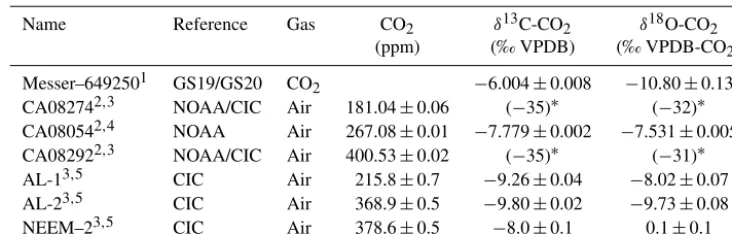
Table 1.Characteristics of published and recently operated analytical systems allowing measurement of CO2mixing ratios and the CO2 stable isotopic composition on a single ice sample. Indicated precisions (1σ )are estimated from replicate analysis of natural ice samples. One should note that the thereby applied metric may not be entirely comparable (e.g. replicates either measured on different or on the same day).
Laboratory Extraction principle Operating Sample mass Extraction efficiency for Daily sample Precision Precision
(design) temp. (◦C) (g) bubbly (clathrate) ice throughput CO2(ppm) δ13C (‰)
KUP mechanical
(NC)
−20 (−35)∗ 5–6 ∼70 (∼50) % 3–6 2.0 0.07
sublimation ∼30 ∼100 (∼100) % 1–2 ∼2.0 0.05
LGGE mechanical
(ball mill)
−65 40–50 ∼70 (not reported) % 1–2 1.5 0.1
OSU mechanical
(cheese grater)
−60 400–550 ∼60 (< 60) % 1–2 1.9 0.02
CSIRO mechanical
(cheese grater)
−20 800–1000 60–80 (unknown) % 3–4 1.0 0.04
CIC (this study) mechanical (NC)
−45 8–13 70–80 (∼60) % 3–4 2.0 0.11
∗Initially reported at−20◦C, but lowered to−35◦C since (Leuenberger, 2009).
CSIRO uses a cheese grater for mechanical extraction (Etheridge et al., 1996; MacFarling Meure et al., 2006; Ru-bino et al., 2013). The released air is cryogenically collected in an external trap (around −260◦C) after removing wa-ter at−100◦C. Subsequently, the sample is analysed using GC for determination of the CO2mixing ratio and by IRMS
for δ13C without further GC separation and purification. A correction for the isobaric N2O interference is applied.
In-terference from drilling fluid contamination can potentially be a problem for certain samples. The large sample size al-lows measurement of other trace gases from the same sample (CH4, CO, and N2O).
In this study, we present a new system built at the Centre for Ice and Climate (CIC, University of Copenhagen, Den-mark) in the laboratory for atmospheric trace gas measure-ments in ice cores (Stowasser et al., 2012; Sperlich et al., 2013). The approach was to opt for small sample size, to allow simultaneous analysis of both CO2mixing ratios and
its stable isotopic composition in the same sample, and to achieve high precision with reasonable throughput in order to pursue high resolution sampling schemes. We thereby fol-lowed the extraction principle of the NC using a modified design. Due to the intended small sample size, the extrac-tion unit was coupled to a continuous flow GC–IRMS set-up, with the benefit of overcoming the problem of interference from isobaric N2O and fragments of remaining
contamina-tion from drilling fluid.
2 Instrumental set-up and standards
2.1 Dry extraction unit
The dry extraction unit was designed based on the NC prin-ciple for small sample sizes of a few grams described by e.g. Lüthi (2009) and Ahn et al. (2009). However, some
ma-jor modifications were implemented to achieve the following goals: (i) avoidance of mechanical friction within the sys-tem in order to reduce related contamination and adsorp-tion/desorption effects (Zumbrunn et al., 1982; Stauffer et al., 1985; Lüthi, 2009); (ii) operation at very low tempera-tures to reduce the risk of CO2in situ production (within the
extraction unit) from chemical reactions due to the presence of H2O in the mobile phase; (iii) fast and simplified sample
loading with minimal exposure of inner surfaces to ambient air in order to maximize sample throughput and to reduce artefacts from surface effects, respectively.
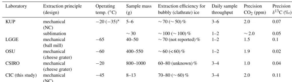
Our NC design for ice samples with maximum dimen-sions of 2.3×2.5×2.5 cm3and a typical mass of 8–13 g is shown in Fig. 1. All inner parts are made from stainless steel (SS). Similar to Ahn et al. (2009), we use a compressible welded bellow (SS, Comvat, Germany, 5 in Fig. 1). This al-lows crushing of the ice by axial movement of the needles mounted with a hot/cold press fit (hardened SS, 1.5 mm OD, 30 mm length, Dema, Germany, 6 in Fig. 1). In comparison to the design described by Lüthi (2009), which requires a vacuum tight seal around a movable piston, the mechanical friction within our unit is thus strongly reduced. In addition, the bellow is mounted differently than in the design presented by Ahn et al. (2009), resulting in an inner volume of half the size (∼110 cm3;∼63 cm3with the bellow compressed) and an inner surface area reduced by about two-thirds. A small volume is favourable in terms of evacuation speed and time required for transferring the gas out of the extraction unit for subsequent treatment. A small inner surface reduces the po-tential for surface effects (adsorption/desorption) which can bias the CO2stable isotope ratios due to isotopic
1a 3a
3a
4a
5
3b
13
7
4b
8 1b
6
3b 10
2a
9 8
11
2b 12
(a) (b)
Figure 1. (a)Schematic of the CIC needle cracker (NC) dry ex-traction unit and(b)picture with cooling jacket and insulation dis-mounted at the top part. Pneumatic actuators (1a, 1b), guiding SS rods with bearings (2a, 2b), cold air inlet and outlet for cooling (3a and 3b respectively), cooling jacket and cooling cavities (4a and 4b, respectively), SS welded bellow (5), SS needle pins (6), ice sample (7), insulation (8), temperature sensor (9), indium wire for vacuum seal (10), gas inlets (11, 12) and outlet (13) equipped with valves.
13 in Fig. 1). A fixed soft copper seal connects the needle piston to the bellow base plate.
Both the crushing mechanism by axial compression of the bellow and the opening/closing mechanism are pneumati-cally actuated. To crush the ice sample, a pressure of 4.7 bar is applied to the upper cylinder (CP95SDB40–80, SMC, 1a in Fig. 1) and the needles are actuated via a 5-port solenoid valve (VQZ3120–5YZB–C10, SMC) controlled by an exter-nal logical device (homemade). The total number and fre-quency of strokes can be controlled and were typically set to 37 and∼3 Hz, respectively. Six bars of air pressure applied on the lower actuator (C95NDB80–250, SMC, 1b in Fig. 1) creates enough force for a vacuum tight sealing between the connection of the upper and lower part of the extraction unit using indium wire (1.5 mm OD, 99.99 %, Sigma-Aldrich, USA, 10 in Fig. 1). Although the wire needs to be replaced whenever a new sample is loaded, the indium can be reused when drawn into wire again. This sealing mechanism reduces the amount of time required to open and vacuum seal the ves-sel compared to systems using bolts and nuts. It takes less than 2 min, including the removal of previously crushed ice, cleaning and reloading of a new sample. To minimize con-tact of ambient air with the inner surfaces and avoid conden-sation/deposition of water vapour, both the lower and upper part of the device are flushed through the respective inlets
with N2(99.999 %, Air Liquid, Denmark) whenever the
sys-tem is opened.
To cool the well-insulated NC, we chose to use an air cooling set-up similar to that described by Schmitt (2006) instead of using a liquid cooling fluid. Pressurized air with an adjustable flow between 0 and∼60 L min−1 is dried in two sequential traps (filled with Molecular sieve 13X/4Å, Su-pelco, USA) and cooled in a copper heat exchanger mounted in a Dewar (D2). D2 is supplied with droplets of liquid ni-trogen (LN) from a larger Dewar (D1) containing the LN reservoir. The droplets are pumped by applying 12.8 V to a heater (10resistor) mounted in the widened inlet of an empty 1/4 in. tube submerged in the LN. Whenever heat is applied, LN evaporates around the heater and the evolving N2
bubbles transport the above, still liquid nitrogen through the isolated tube to D2. This LN pump is regulated by the use of two coupled proportional–integral–derivative controllers (PID, iTRON 08, JUMO, UK). One PID is set to the desired final temperature measured in the NC (9 in Fig. 1), whereas the other is set to a minimum temperature of−180◦C in D2, preventing the system from eventual clogging by frozen rem-nant water in the air stream and from potential condensa-tion of oxygen. The temperatures used for PID input and sur-vey of the air stream are measured with platinum resistance thermometer PT100 elements (100,−200 to 600◦C, Class 1/10, TC Direct, USA). By changing the settings for air flow and/or the set points for NC and D2, the air stream tempera-ture is regulated. To cool the NC, the cold air stream is split in front of the unit and either directed through the cavities in the lower part of the massive steel unit (4b in Fig. 1) or the cool-ing jacket mounted around the compressible welded bellow (4a in Fig. 1). The minimum operating temperature of the NC is−55◦C, whereas the standard operating temperature
is set to−45◦C (stability±1◦C) with significantly reduced build-up of ice on the vacuum sealing surfaces. While cool-ing down to−45◦C, the air stream first regulates to about
−80◦C before it stabilizes at −60◦C. Cooling the NC to
−45◦C takes around 70 min.
Compared to other systems allowing analysis of similarly small sample sizes (other NC designs, CIM) the operating temperature of our extraction chamber is significantly lower (−45◦C compared to around −35/−30◦C). This is benefi-ciary because the resulting lower water partial pressure in the extraction chamber (about 5-fold) reduces the risk of in situ CO2 production by wet chemistry. This is supported by the
LN2
GC-2 35 °C CF -196 °C
Open split Ref. port (WS on/off)
Ion source
Farraday cups m/z 44 45 46
IRMS Delta V Plus Nafion dryer He
20 mL min He
10 mL min
He 10 mL min
He 7 mL min He (discharge)
30 mL min He (reference)
10 mL min
LN2
LN2
WS-CO2
CO He
PDD TCD
GC-1 30 °C
injV
V2 V3
V1
HV LV WT
-196 °C LN2 Extraction (NC)
T1 Ice
Cooling (dried air, -80 °C) DF
(11 cm3)
Heating -45 °C, 63 – 110 cm3 Vacuum line, gas manifold, extraction
N2 He 80 mL min
T3 -196 °C
100 °C -196 °C
150 °C
He 1.5 mL min
P1
P2
Air sample
T2 -196°C
150°C
GC separation, detection (continuous flow, automated)
(a) (b)
Trace GC Ultra Gas manifold
Vacuum line
GP interface 3-WV
Air STD
12
11 13
14
15
–1
–1
–1 –1
–1
–1
–1
–1 Air STD
Air STD Air STD Air STD Air STD
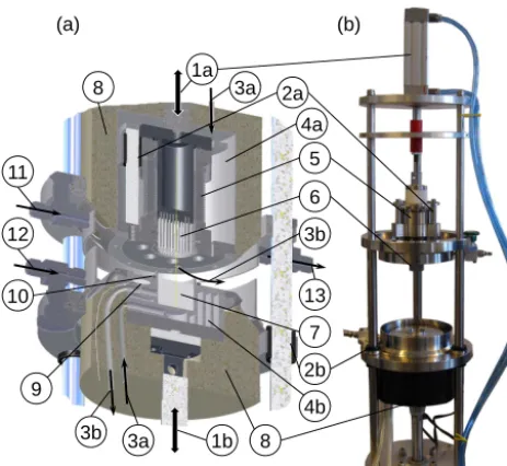
Figure 2.Schematic representation of the new analytical CIC system for simultaneous measurements of CO2mixing and stable isotope
ratios. The set-up consists of a manually operated section A, allowing injection and loading of air and ice samples, and a fully automated section B, for gas separation, purification and final detection run in continuous flow mode. Highlighted in red and green are components for gas separation and detection, respectively. See main text for details (Sects. 2 and 3).
2.2 Analytical system
Our analytical system allows simultaneous measurements of atmospheric CO2mixing ratios and its stable isotopic
com-position in the same sample. A schematic representation of the system is shown in Fig. 2. It can be divided into two main sections: section A (manually operated) for standard or sam-ple gas loading, and section B (fully automated and in con-tinuous flow mode) for gas separation (PreCon) and injection into the detection systems.
Section A consists of four main parts: i. a vacuum line;
ii. a gas manifold for carrier-, protection- or standard-gas injection;
iii. a dry extraction unit (NC);
iv. a trap (T1) to quantitatively cryopump sampled gas out of the NC for subsequent and complete transfer from section A to B.
Section B consists of two main parts:
i. a gas separation part which allows initial trapping of the transferred sample (T2), separation of CO2 (and N2O)
from the major air components (T3) and subsequent par-titioning of the two fractions to individual lines for ei-ther final detection (main air fraction) or furei-ther purifi-cation by gas chromatography (GC–1 and GC–2);
ii. the detection systems including a thermal conductivity detector to quantify the amount of the main air fraction (TCD, VICI, USA, integral part of GC–1, TRACE GC Ultra, Thermo Scientific, USA), a pulsed discharge de-tector to survey CO2separation and purification (PDD,
VICI, USA, integral part of GC–1) and an IRMS to quantify amount and isotopic ratios of the CO2fraction
(Delta V Plus, Thermo Fisher, Germany).
All inner surfaces of the set-up are either made from SS or fused silica and the connections are either welded or sealed with metal or graphite/vespel ferrules to exclude artefacts due to outgassing (Sturm et al., 2004). Section A can either be evacuated or flushed with N2(inert gas also used for
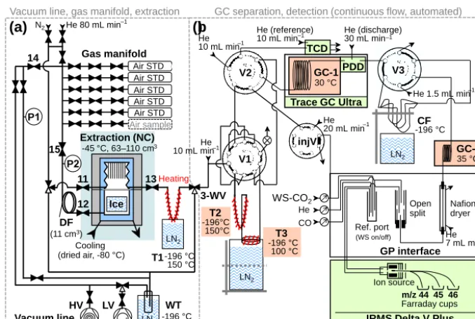
Table 2.CIC reference standards for CO2mixing and stable isotope ratios.
Name Reference Gas CO2 δ13C-CO2 δ18O-CO2
(ppm) (‰ VPDB) (‰ VPDB-CO2)
Messer–6492501 GS19/GS20 CO2 −6.004±0.008 −10.80±0.13
CA082742,3 NOAA/CIC Air 181.04±0.06 (−35)∗ (−32)∗ CA080542,4 NOAA Air 267.08±0.01 −7.779±0.002 −7.531±0.005 CA082922,3 NOAA/CIC Air 400.53±0.02 (−35)∗ (−31)∗
AL-13,5 CIC Air 215.8±0.7 −9.26±0.04 −8.02±0.07
AL-23,5 CIC Air 368.9±0.5 −9.80±0.02 −9.73±0.08
NEEM–23,5 CIC Air 378.6±0.5 −8.0±0.1 0.1±0.1
1Stable isotopic composition calibrated at CIC by IRMS dual-inlet against GS19 and GS20 (Centre for Isotope Research,
Gröningen University, Netherlands).2CO2mixing ratio calibrated and certified by NOAA ESRL/GMD (Boulder, Colorado,
USA).3Stable isotopic composition calibrated at CIC against Messer–649250 and CA08054 with the set-up described in this study but in “dry mode” (without ice).4Stable isotopic composition calibrated by the Stable Isotope Lab at INSTAAR (SIOL, University of Colorado, USA) in cooperation with NOAA.5CO2mixing ratio calibrated at CIC against the three NOAA
standards CA08274, CA08054 and CA08292, with the set-up described in this study and by WS-CRD spectroscopy.∗Values outside of the reliable calibration range.
2.3 Standards
The reported CO2mixing ratios (also referred to as CO2
con-centrations in the literature) are defined as the dry air mole fraction expressed in parts per million by volume (ppm), and are linked to the World Meteorological Organization (WMO) mole fraction scale for CO2 in air (Tans and Zhao, 2003;
Zhao and Tans, 2006). Isotope ratios are reported relative to the international measurement standards (VPDB, VPDB-CO2and VSMOW for13C-CO2,18O-CO2and18O-H2O,
re-spectively) using the delta notation:
δ=
R
sample
Rstandard
−1, (1)
where R denotes the ratio of the heavy to light isotope in the sample and the standard, respectively. Our working stan-dards were selected in order to cover the range of atmo-spheric CO2 mixing and stable isotope ratios expected for
glacial to interglacial conditions (Table 2). With these stan-dards, system characterization, daily calibration and contin-uous quality control sample (QCS) measurements were per-formed (Sects. 3 and 4).
For referencing IRMS measurements, a working standard (WS) of pure CO2from a natural source (Messer–649250,
Messer, Italy) is injected via an open-split interface (GP interface). Its stable isotopic composition was referenced at CIC against pure CO2 reference gases GS19 and GS20
from the Centre for Isotope Research (Gröningen Univer-sity, Netherlands; Meijer, 1995) by IRMS dual-inlet mea-surement (Delta V Plus, Thermo Fisher, Germany). For air standards we used three synthetic air mixtures, in the fol-lowing called CA08274, CA08054 and CA08292 provided by the Global Monitoring Division of the Earth System Re-search Laboratory at the National Oceanic and Atmospheric Administration (NOAA ESRL/GMD, Boulder, USA), two pressurized air tanks called AL-1 and AL-2 (Air Liquid,
Denmark) and one of two atmospheric air tanks sampled in 2008 at a clean-air site of the NEEM deep ice core drilling camp called NEEM–2. The three NOAA tanks have been calibrated and certified by the NOAA ESRL/GMD Carbon Cycle Gases Group for CO2mixing ratios. The other tanks
have then been calibrated against these three standards at CIC both with the set-up described in this study and di-rectly from the tanks by wavelength-scanned cavity ring-down spectroscopy (WS-CRDS; CFADS36 CO2/CH4/H2O
analyser, Picarro Inc., USA). The stable isotopic composi-tion of CA08054 has been calibrated by the Stable Isotope Lab at INSTAAR (SIOL, University of Colorado) in coop-eration with the NOAA Climate Monitoring and Diagnostics division (CMDL). The stable isotopic composition of the two other NOAA cylinders and of AL-1, AL-2 and NEEM-2 has been calibrated at CIC against Messer–649250 and CA08054 with the set-up described here. All tanks were equipped with high-purity regulators (Y13–C444A, single stage, stainless steel with Kel–F and Teflon seals, Airgas, USA).
3 Measurement procedures and quality control
3.1 PreCon system
The pure CO2-WS (Messer–649250) is injected via an
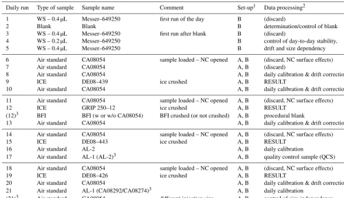
Table 3. Example of a daily measurement sequence. See Table 2 for details on standard gases (WS, air standard) and the main text for analytical procedures. BFI denotes bubble-free ice.
Daily run Type of sample Sample name Comment Set-up1 Data processing2
1 WS – 0.4 µL Messer–649250 first run of the day B (discard)
2 Blank Blank B determination/control of blank
3 WS – 0.4 µL Messer–649250 first run after blank B (discard)
4 WS – 0.2 µL Messer–649250 B control of day-to-day stability,
5 WS – 0.4 µL Messer–649250 B drift and size dependency
6 Air standard CA08054 sample loaded – NC opened A, B (discard, NC surface effects)
7 Air standard CA08054 A, B (discard)
8 Air standard CA08054 A, B daily calibration & drift correction
9 ICE DE08–439 ice crushed A, B RESULT
10 Air standard CA08054 A, B daily calibration & drift correction
11 Air standard CA08054 sample loaded – NC opened A, B (discard, NC surface effects)
12 ICE GRIP 250–12 ice crushed A, B RESULT
(12)3 BFI BFI (w or w/o CA08054) BFI crushed (or not crushed) A, B procedural blank
13 Air standard CA08054 A, B daily calibration & drift correction
14 Air standard CA08054 sample loaded – NC opened A, B (discard, NC surface effects)
15 ICE DE08–443 ice crushed A, B RESULT
16 Air standard AL-2 A, B daily calibration
17 Air standard AL-1 (AL-2)3 A, B quality control sample (QCS)
18 Air standard CA08054 sample loaded – NC opened A, B (discard, NC surface effects)
19 ICE DE08–426 ice crushed A, B RESULT
20 Air standard CA08054 A, B daily calibration & drift correction
21 Air standard AL-1 (CA08292/CA08274)3 A, B daily calibration
(21)3 Air standard CA08054 different injection size A, B control of size independency
1Section of system passed by the analysed gas sample (see Fig. 2).2See main text for details about data processing.3Alternative measurement option.
The following step by step description of the measurement procedure follows part numbering and abbreviations as in-dicated in Fig. 2. Connected in series, the cryogenic traps T2 (1/4 in. SS Swagelok tube, filled with around 5 cm of HayeSep D, 100/120 mesh, Sigma-Aldrich, Switzerland) and T3 (empty 1/16 in. SS Swagelok tube) are cooled by be-ing immersed into liquid nitrogen. In order to prevent am-bient air to be sucked into these traps while cooling down, the on/off valve (SS–4BK–TW–1C, Swagelok, USA) at the vent is closed. Then, various amounts of pure CO2-WS are
injected directly onto T2 with valve V1 (10-port, 1/8 in., air actuated, A210UWM, VICI, USA) switched compared to Fig. 2. To vary the injected amount an internal sample injec-tion valve with a defined volume of 0.1 µL is switched for the selected number of times (injV, AN14WM.1, VICI, USA). Alternatively, if the valve is not switched, only helium car-rier gas is passed through the system (20 mL min−1, set by a flow controller, Model VCD 1000, Porter, USA) and a blank measurement for this section of the system is obtained. In any case, V2 (6-port, 5UWM, VICI, USA) is switched after a trapping time of 6 min – similar to the trapping time applied for air standard and ice sample measurements – directing the sample gas flow (10 mL min−1 set by a flow controller; VCD 1000, Porter, USA) through the TCD detector. After an
idle time of 30 s allowing the flow to stabilize, the LN De-war cooling T2 and T3 is automatically lowered by a double activated pneumatic cylinder (CD85N20–250B, SMC, Den-mark) to a level at which T3 is still cooled. T2 is then heated by a rope heater (FGR–060, Omegalux, UK) to the set tem-perature of 150◦C regulated by a PID controller (iTRON 08, JUMO, UK). Thereby, the trapped gas is released and the amount of the main air components is detected by the TCD (no signal for pure CO2and for blanks) while both CO2
and N2O are trapped in T3 for later separation and detection
in a second line (typical chromatograms for measurements of CO2-WS, procedural blanks and ice core samples can be
found in Supplement Figs. S1 and S2 and in Fig. 3, respec-tively). After 5 min, V2 is switched again, now redirecting the sample flow (again 20 mL min−1)through this alterna-tive detection line. After an idle time of 40 s allowing the flow to stabilize, the LN Dewar is further lowered and trap T3 quickly heated to 100◦C (resistance wire, 2.5m−1, 5 m, Conrad Electronics, Germany) regulated by a second PID controller (iTRON 32, JUMO, UK). Thereby, CO2and N2O
(not present in the pure CO2-WS) are released and the
6.479 3.138901 0.001916 0.004557 0.003139
6.688 1.904664 3.146572 0.001905 0.00457 0.003147
6.896 1.910405 4.564426 3.108218 0.00191 0.004564 0.003108
7.105 1.918061 4.595199 3.125476 0.001918 0.004595 0.003125
7.315 1.914233 4.612511 3.117806 0.001914 0.004613 0.003118
7.524 1.914233 4.574042 3.104383 0.001914 0.004574 0.003104
7.732 1.912319 4.525965 3.123559 0.001912 0.004526 0.003124
7.941 1.927631 4.579812 3.117806 0.001928 0.00458 0.003118
8.151 1.919975 4.608664 3.154243 0.00192 0.004609 0.003154
8.359 1.923803 4.604817 3.112053 0.001924 0.004605 0.003112
8.569 1.919975 4.585582 3.14849 0.00192 0.004586 0.003148
8.777 1.912319 4.602893 3.094795 0.001912 0.004603 0.003095
8.987 1.910405 4.572119 3.110135 0.00191 0.004572 0.00311
9.196 1.923803 4.593276 3.13123 0.001924 0.004593 0.003131
9.404 1.918061 4.579812 3.179178 0.001918 0.00458 0.003179
9.614 1.916147 4.556733 3.236727 0.001916 0.004557 0.003237
9.822 1.910405 4.574042 3.154243 0.00191 0.004574 0.003154
10.031 1.914233 4.593276 3.089043 0.001914 0.004593 0.003089
10.241 1.897009 4.520196 3.104383 0.001897 0.00452 0.003104
10.449 1.904664 4.545195 3.057445 0.001905 0.004545 0.003057
10.659 1.919975 4.568273 3.112053 0.00192 0.004568 0.003112
10.868 1.914233 4.552887 3.152326 0.001914 0.004553 0.003152
11.076 1.914233 4.620205 3.096713 0.001914 0.00462 0.003097
0 2 4 6 8
In
te
n
si
ty
(V
)
m/z 44 m/z 45
0 1 2 3 4
0 200 400 600 800 1000 1200
In
te
n
si
ty
(V
)
Time (s)
PDD TCD
0.0 0.1 0.2
700 750 800 850
CO2
N2
Valve switching
GC-1 T increase
O2 CO2
0 0.04 0.08
1020 1070 1120
N2O N2O N2O
CO2 CO2 CO2
CF in / out (3x) Air
N2O
Drilling fluid H2O
1 2 3 4 5 6 7 8 9 10
11 12 13 14
m/z 46
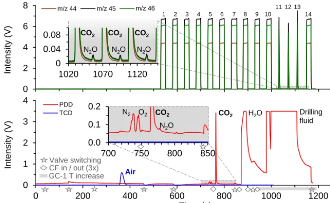
Figure 3.Chromatograms for the measurement of an ice sample as described in Sect. 3.2. Upper panel: IRMS signal intensity form/z44, 45 and 46. Injections of the WS via the open split are identifiable by the flat-topped peaks. Peaks 1–9 are used to reach stable source conditions while peaks 10 and 14 before and after the samples are used for referencing. The inset shows baseline details and N2O separation in detail.
Lower panel: PDD and TCD intensity signal for CO2and air, respectively. Stars indicate valve switching, resulting in small variations in the
PDD signal due to changes in pressure and flow (see inset, not detected by the less sensitive TCD). Diamonds indicate immersion of the three capillary traps into liquid nitrogen for CO2cryofocusing and their subsequent one-by-one release resulting in the three peaks of the split
sample shown in the upper panel (peaks 11–13). Over the time period, indicated by the grey bar, the GC–1 temperature is increased to 150◦C in order to precondition the column for the next sample (release of water and remnants of drilling fluid contamination). The enlargement shows baseline details revealing the N2O peak and small remains of N2and O2from the air sample, incompletely separated by the preceding cryogenic partition.
USA). The signal then being detected by the PDD is shown in Fig. S1 (Supplement). Shortly before the eluted CO2peak
arrives at the PDD (discharge gas flow set to 30 mL min−1), three parallel traps (fused silica capillaries, 250 µm ID, 1.8 m length, BGB, Germany) are immersed into LN to re-trap CO2
and N2O for cryogenic focus (CF) after splitting the sample
stream at the PDD outlet valve V3 (GC built in 6-port valve, VICI, USA). To vent remaining H2O and potential
contami-nants from drilling fluid (for ice samples), V3 is switched be-fore the signal is detected in the PDD (∼70 s after the max-imum in the CO2peak). The GC column is then conditioned
for the next sample by heating to 150◦C. In the separated part of the line, the three CF capillaries are meanwhile lifted one after the other out of the LN, subsequently releasing the sample – now split in three aliquots – for further transport in a reduced He flow of 1.5 mL min−1. To avoid isobaric interfer-ence, CO2and N2O contained in these aliquots are again
sep-arated in a second GC column (GC–2; 35◦C, CP–PoraBond–
Q, 40 cm×0.53 mm ID, df =10 µm, Varian, USA) before the remnant water vapour is removed by a Nafion drying column (40 cm×0.36 mm ID , Perma Pure Inc., USA). Fi-nally, the sample gases are introduced to the IRMS via the open split of the GP interface. Before the three CO2
sam-ple peaks elute, the reference gas (CO2-WS, here the same
as the sample gas) is injected several times (reference port)
in order to reach stable IRMS-source conditions. The peak amplitude is thereby adjusted to closely match the amplitude of the sample aliquots (not for blanks). For the same reason a constant CO background flow through the reference open-split port into the ion source was maintained as proposed in Elsig and Leuenberger (2010). The mean value of the peak before and after the sample is ultimately used for referenc-ing. Splitting the sample in aliquots allows for three IRMS measurements on the same sample theoretically improving the analytical precision. In practice, the therefore required quantitative splitting in three evenly sized aliquots is diffi-cult to achieve. For the calculated mean values (weighted by mass, i.e. size) no difference in final precision compared to a single measurement was observed. However, results from these multiple measurements could be statistically analysed and were useful, e.g., to evaluate the applied IRMS nonlin-earity correction which reduces the standard deviation over the three replicates (Sect. 4.1.2).
3.2 Standard air, ice samples and blanks
Air standards and blank measurements were performed regu-larly for calibration and system characterization, thereby fol-lowing the exact procedure used to measure real (natural) ice samples, i.e. following the “identical treatment” principle (Werner and Brand, 2001). To simulate the entire measure-ment procedure as close as possible, artificial bubble-free ice (BFI) samples were used. BFI was produced from ultrapure water (MilliQ, 18.2Mcm at 25◦C) degassed for 60–90 min using a roughing LV pump (E2M0.7, Edwards, UK) and then slowly frozen from the bottom (20 cm in 48 h), thereby forc-ing the remainforc-ing gas out of the water. Results for calibra-tions and system characterization will be presented in Sect. 4. Samples of air, either from tanks (e.g. atmospheric sam-ples or standards) or extracted from ice core samsam-ples, pass all sections of the experimental set-up (A and B, Fig. 2). When the system is not in use (e.g. overnight), section B is constantly flushed with He while all lines in section A and the NC are pressurized slightly above atmospheric pressure with He and N2, respectively. Prior to analysis, ice core or
BFI samples are cut to the required dimensions and the sur-faces are decontaminated by removing the top layers with a scalpel.
A typical daily measurement sequence is listed in Table 3. The measurements can be separated into five main cate-gories:
1. air standard measurements performed by injecting vari-able amounts of the standard gas over an ice sample of either natural or artificial origin (BFI) without crushing the ice; standards of different CO2 mixing ratios and
isotopic composition were thereby used (Table 2); 2. system blank measurements performed by omitting
ad-dition of standard gas and hence resulting in sampling carrier gas only;
3. BFI measurements either performed with air standard added or omitted but with the ice being crushed; 4. measurements simulating the crushing procedure (i.e.
needles moved) but using BFI which has been crushed in advance; in this case, artefacts from remnant gas po-tentially present in the initial, intact BFI sample can be excluded (Sect. 4); these measurements were also per-formed with and without the addition of air standard; the latter case will be further referred to as “procedural blank”;
5. measurements of air extracted from natural ice samples by crushing the ice.
The following step by step description of the measurement procedure follows part numbering and abbreviations as indi-cated in Fig. 2. Section A and the NC are prepared for mea-surements during the first five runs of the daily sequence (Ta-ble 3). The procedure for these runs is described in Sect. 3.1.
After the air cooling system of the NC is started, the first ice sample is loaded once a temperature of−20◦C has been
reached. While the unit is open, both the upper and lower parts are continuously flushed with N2through the respective
inlets (11 and 12) to prevent contamination from ambient air and condensation of water vapour on the cold inner surfaces. After the NC is closed and vacuum sealed again, inlets 11 and 12 are closed and the N2flow is turned off.
Each time the NC is opened, the following sequence of steps is required for evacuation and reconditioning. The chamber is evacuated by the LV pump through inlet 11 for 1 min. Only port 11 is used in this evacuation step to pre-vent trapping of N2on trap T1 (heated to 100◦C, 1/4 in. SS
tube, filled with HayeSep D, 100/120 mesh, Sigma-Aldrich). This is essential because at this point the N2 abundance in
the NC is much higher than in samples of recent or past at-mosphere. When the system is evacuated, inlet 12 remains always closed. To avoid analytical artefacts, this inlet is only used with a one-directional flow into the NC, thus preventing water vapour from reaching the gas manifold and the vacuum lines used for the injection of standard air samples. When the pressure in the NC has dropped, trap T1 and the rest of the vacuum lines still filled with He or N2, respectively, are now
also evacuated through the respective lines. After a few sec-onds the vacuum system is switched to the HV pump for an-other 5 min. To precondition the NC, the chamber is closed off from the vacuum (valves 11 and 13) and then filled with an aliquot of air standard through inlet 12. Since the standard added in this step is used only for conditioning, the injected amount is non-quantitative. After inlet 12 is closed again, T1 is cooled down by being immersed in LN before outlet 13 is opened to cryogenically pump the air aliquot onto T1. After a trapping time of 3 min, the line (vacuum line–NC–T1) is flushed with He from the inlet next to the gas manifold set to a flow of 80 mL min−1(gas flow controller, Model 100, VICI, USA). Since this air aliquot is not to be analysed, the He gas flow is then directed through the 3-way valve (3-WV; SS–43GXS4, Swagelok, USA) into the LV pump. To release the previously trapped air sample while flushing, T1 is heated by a rope heater (FGR–060, Omegalux, UK) to the set tem-perature of 150◦C regulated by a PID controller (N2300, West Instruments, USA). After a flushing time of 3 min, out-let 13 and inout-let 12 are closed and the temperature of T1 is reduced to 100◦C. The system is now in a similar state as prior to runs where the NC has not been opened beforehand (see Table 3).
expansion step, an equilibrium time of 2 min was applied. In every sequence, the first run which includes section A (run 6) is performed using an air standard of large size (aliquot expanded from the volume between the first and last valves of the gas manifold line). This allows for a first immediate control of system conditions and day by day stability after the idle time overnight. From the gas manifold the sample is expanded into a defined volume of∼11 cm3(DF), equipped with another pressure gauge, P2 (high-precision piezo pres-sure transmitter, PAA–35X, Keller AG, Switzerland). After DF has been closed off towards the manifold (valve 15) and the NC (inlet 12 has been closed initially), the pressure is recorded for later use (Sect. 4.1.1). At the same time, sam-ple air contained in the rest of the lines is pumped off by the HV pump. After the pressure has been recorded and valves 11 and 13 have been closed, the gas is further expanded into the NC. The standard gas is kept in the NC for 2 min, sim-ulating the procedure applied for natural ice samples which are crushed at this point, allowing the gas to subsequently expand from the ice. The valve to DF is thereby kept open, which allows us to record and survey the efficiency of gas extraction from the opened bubbles when measuring natu-ral ice samples and subsequently the gas transfer out of the NC onto the pre-cooled trap T1 in the following 3 min cryo-genic pumping step. Afterwards, with the cryopump still ac-tive (i.e. T1 still cooled with LN), the NC and T1 are filled with He (80 mL min−1)to 1100 mbar, which is slightly above the pressure in section B (∼3 min). This prevents backflush-ing from section B to A when they are connected by switch-ing the 3–WV. At this point, the air sample is released by heating T1 to the set temperature of 150◦C and transferred to the pre-cooled trap T2 by the carrier gas (80 mL min−1). This step takes another 3 min. The 3–WV is then closed, again separating section A and B. From here on, the sample is in a reduced carrier gas flow environment, and further sample treatment is handled by the automated part of the system as described in Sect. 3.1. Meanwhile section A can be prepared for the next sample. Therefore, the outlet valve of the NC is closed, the N2 flush flow opened and the next ice cube
loaded. If the next sample in the sequence (Table 3) is to be measured with the ice remaining in the NC, evacuation of the extraction unit and the vacuum lines is sufficient to prepare for the next run.
For the measurement of natural ice samples, the procedure is as described above but all steps related to the air standard addition can be skipped. Chromatograms of the TCD, PDD and IRMS for a typical ice sample measurement are shown in Fig. 3. Here, as opposed to measurements of pure CO2-WS
and blanks (Figs. S1 and S2, respectively), the peak from sample air shows up as a distinct TCD signal, and signals of H2O from ice sample water vapour and remnants of drilling
fluid contamination are detected by the PDD in addition. Including section A of the system does not add much to the total measurement time given in Sect. 3.1 because most of the additional steps required can already be executed while
the current measurement is running in the automated sec-tion B. Typically, the analysis takes around 30 min (run to run). However, it increases for runs requiring loading of a new ice sample (opening of the NC) and as a consequence the described evacuation and flushing steps (∼50 min, e.g. runs 6, 11, 14 and 18 in Table 3).
4 Results and discussion
4.1 Evaluation and calibration
System-specific analytical bias for CO2 concentration and
CO2stable isotope measurements can result from
fractiona-tion in the analytical system related to adsorpfractiona-tion and desorp-tion processes, specifically in the extracdesorp-tion unit (Zumbrunn et al., 1982), non-quantitative trapping and releasing of gas and from GC separation. For stable isotope measurements, further bias arises from IRMS injection and source effects (Elsig and Leuenberger, 2010). The net effect of these pro-cesses was assessed and monitored on a regular basis to ac-count for system drifts. Such drifts may occur when bound-ary conditions (e.g. room temperature) change and can ap-pear within a measurement day, on a day to day basis and on longer timescales, here being either related to changes in the set-up (e.g. replacements of parts, change of carrier gas tanks or standards, adjustments in carrier gas flows) or small changes in the procedure. Following the identical treatment principle (Werner and Brand, 2001), we characterized all sec-tions of our system for systematic effects using the various standards available (Table 2), ultimately allowing a reliable correction of the raw data. Runs of QCS to assess long-term stability of our final measurement results were carried out on a daily basis (results in Sect. 4.2.1).
4.1.1 CO2
CO2mixing ratios can, in principle, be derived from the ratio
between the IRMS CO2peak area (values given in the
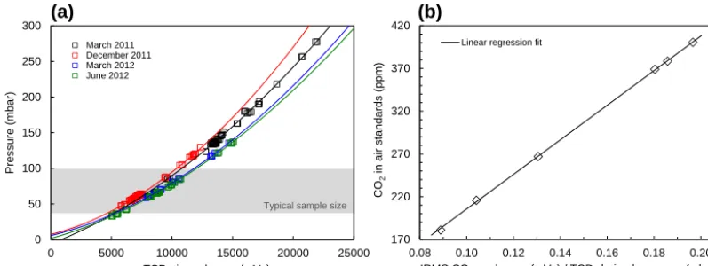
fol-lowing always denote the mean for the three sample peaks) and the major air components detected as TCD peak area (Fig. 3). The TCD air peak signal was observed to be nonlin-early related to the amount of air with significant variability. This can be seen in the relation between the high-precision pressure readings of standard gas (described in Sect. 3.2) and the TCD air peak area investigated for different measument periods (Fig. 4a). We also found variability in the re-lation between the IRMS peak area and the CO2amount; in
this case, however, the relationship is linear. Reasons for the observed variability are manifold, e.g. small adjustments in flow or trapping procedures, or small changes in outer condi-tions such as room temperature (e.g. March and June 2012).
0 50 100 150 200 250 300
0 5000 10000 15000 20000 25000
Pr
e
s
s
u
re
(
m
b
a
r)
TCD air peak area (mVs)
March 2011 December 2011 March 2012 June 2012
Typical sample size
(a) (b)
170 220 270 320 370 420
0.08 0.10 0.12 0.14 0.16 0.18 0.20
C
O2
in
a
ir
st
a
n
d
a
rd
s
(p
p
m
)
IRMS CO peak area (mVs) / TCD-derived pressure (mbar)2
Linear regression fit
Figure 4.CO2calibration.(a)Relationship between sample size and TCD peak area of air for different measurement periods. The lines are
second-order polynomial fits through the data. Pressure in the injection volume is proportional to amount. The grey bar indicates the typical sample size range extracted from ice samples.(b)Calibration curve; known CO2mixing ratios of air standards vs. ratio of IRMS peak area
for CO2(m/z44) and TCD detected air amount transformed to pressure from the relationship shown in(a).
the data obtained from daily performed measurements of air standards. In doing so, the large long-term variations in TCD sensitivity are accounted for and all TCD measurements are adjusted and referred to a common scale (pressure). The CO2
mixing ratios known for the standard gases were then related to the derived ratio between the IRMS CO2peak area and the
computed pressure. By including data of all available stan-dards, the resulting linear calibration curve is well defined over a large concentration range (Fig. 4b). The data shown are based on repeated measurements series over the course of more than 1 year (n=4). Each series was performed on a single day with the entire range of standards being measured at least three times. The ratios calculated for the individual series were matched for CA08054 in order to account for the long-term variation of the IRMS response, resulting in the average transfer function shown.
With the calibration curve covering the entire range of ex-pected measurement results (Fig. 4b), daily calibration could be performed with a subset of standards only, thus signifi-cantly reducing the total sequence time. Summarized in Ta-ble 3, a typical daily measurement sequence includes the re-peated measurement of standard CA08504 (run 8, 10, 13 and 20) to determine and subsequently adjust for (i) potential off-set in the calculated ratio compared to the calibration curve and (ii) system drift over the sequence measurement time. It further includes at least one additional standard gas measure-ment with a different CO2mixing ratio to adjust for potential
variations in the slope of the linear calibration fit (runs 16, 21 and 17 if necessary). If not used in the daily calibration, run 17 is treated as a real sample in the post processing of the raw data, allowing us to assess the long-term consistency and precision of our measurements (QCS; see Sect. 4.2.1). In run 21, CA08504 is occasionally injected in variable amounts to ensure the independence of the final results from the sampled amount of gas.
Procedural blank: We find that independently of sample size, gas amount or CO2concentration, a constant amount of
CO2is produced by the extraction itself. This amount was
de-termined by measurements of BFI samples. To perfectly sim-ulate measurements of natural ice samples according to the identical treatment principle (Werner and Brand, 2001), ar-tificially produced bubble ice with entrapped standard gases would be required. Because this is technically not feasible, instead we added standard gas to a BFI sample loaded in the NC and crushed for the measurement. The CO2mixing
ra-tios we observed were elevated by 4.6±2.6 ppm on average (n=5) compared to the expected value. However, for sub-sequent measurements with an identical procedure (includ-ing movement of the needle pins), but us(includ-ing the previously crushed BFI, the observed elevation was less. This indicates the presence of remnant gases in our BFI which is in agree-ment with independent results from another study (∼3 ppm for CIC BFI, Appendix A6 in Rubino et al., 2013). We thus considered the lower offset value of 2.3±2.0 ppm (average,
n=4) to be representative of the purely system related blank. This is a reduced offset compared to other systems, allow-ing the analysis of similarly small sample sizes (e.g. 4.9 ppm for the KUP NC; Bereiter et al., 2013) which most likely is a result of the friction-reduced motion and lower operat-ing temperature in our NC design. Anyhow, this CO2
enrich-ment – expressed in ppm before – is observed in the raw data as an elevated signal in the IRMS CO2peak area. The size
of this extra signal can therefore be directly estimated from procedural blank measurements when using BFI which has been crushed in advance (Fig. S3). As an advantage, propa-gation of uncertainties associated with data post-processing can then be omitted. Combining the results from both ap-proaches, the IRMS CO2peak area for the procedural blank
Sect. 4.1.2 – Air amount dependence). In Sect. 4.1.3, the pro-cedural blank correction applied to ice core samples will be discussed in detail.
4.1.2 δ13C-CO2andδ18O-CO2
The individual sections of the set-up were characterized for systematic effects on δ13C and δ18O results. Calibrations, control of system stability and blanks, as well as QCS mea-surements to assure the long-term quality of our analysis (Sect. 4.2.1), were all performed on a daily basis (Table 3).
IRMS nonlinearity: We characterized the IRMS source effects – in the following referred to as IRMS nonlinear-ity – by measurements of reference gas (CO2-WS) injected
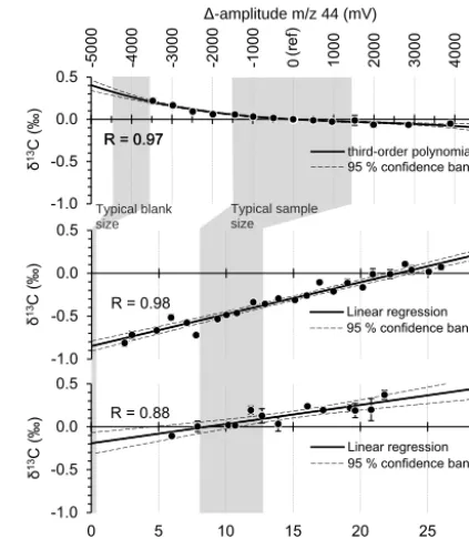
via the GP interface reference open split (Fig. 2). To reach stable source conditions, six injections were made prior to acquisition similar to the approach described in Elsig and Leuenberger (2010). Then, the injection amount was in-creased step-wise, reflected in rising amplitudes of the rect-angular peaks. The signal amplitude thereby ranged between 400 and 8400 mV (m/z 44), with the reference peak al-ways set to around 4000 mV (gain:R=108). This exper-iment was replicated on three different days distributed over a time period of 1 year. The resulting total number of acqui-sitions was 177. In Fig. 5a, the IRMS nonlinearity effect for
δ13C is shown, measured as the deviation from the reference (∼4000 mV). The same procedure was applied to investigate theδ18O nonlinearity (Fig. S3).
PreCon–GC linearity: A potential and possibly size-dependent effect on the stable isotope values of the sampled gas when passing the various traps and GC columns in the automated set-up section B (Fig. 2) was investigated. There-fore, various amounts of the CO2-WS were injected onto
trap T2 via the injV (Fig. 2) as described in Sect. 3.1. The relationship found will be denoted as PreCon–GC linearity in the following. In addition, the blank for this section was determined when injection of CO2 was omitted, but
other-wise the exact same procedure was followed (Sect. 3.1). To allow determination of this PreCon–GC-related effect inde-pendently from any other system-induced contribution, the obtained raw data were first corrected for the IRMS nonlin-earity by applying the third-order polynomial fit shown in Fig. 5a. Subsequently, a blank correction using the values determined here was applied. Therefore, the following equa-tion which closely approximates the isotopic composiequa-tion in a pool (δ6)of isotopically different members (mi with
cor-respondingδi)was used:
δ6= 6 miδi
6 mi
. (2)
Equation (2) shows that the bigger the CO2blank-to-sample
ratio and the difference between blank and sample isotopic composition, the bigger the blank correction will be. In other words, even when the blank is constant both in size and iso-topic composition, the blank correction should vary
depend-R = 0.88
-1.0 -0.5 0.0 0.5
0 5 10 15 20 25 30
δ
13C (‰)
Area m/z 44 (mVs)
Linear regression 95 % confidence band -1.0
-0.5 0.0
0.5 -5000 -4000 -3000 -2000 -1000 0 1000 2000 3000 4000 5000
δ
13C (‰)
∆-amplitude m/z 44 (mV)
third-order polynomial fit
95 % confidence band R = 0.97
R = 0.97
R = 0.98
-1.0 -0.5 0.0 0.5
δ
13C (‰) Linear regression
95 % confidence band
Typical sample size Typical blank
size
(ref)
(a)
(b)
(c)
Figure 5.Fractionation effects for δ13C:(a)IRMS nonlinearity; δ13C dependence on peak amplitude (top x axis),1−amplitude is the deviation in intensity (m/z44) from the reference peak (ref, δ13C and1−amplitude=0). The data are obtained from a total of 177 measurements and mean values with the 1σstandard deviation are shown.(b)PreCon–GC linearity (bottomxaxis); CO2sample
size dependence for pure CO2working standard directly injected to section B. The data are obtained from a total of 318 measurements corrected for IRMS nonlinearity and blank; mean values with the 1σ standard deviation are shown.(c)Air amount dependence (bot-tomxaxis); air sample size dependence for air standards/samples injected to section A. The data are obtained from a total of 46 mea-surements corrected for IRMS nonlinearity, PreCon–GC linearity and system blank. Mean values with the 1σ standard deviation are shown. The grey bars indicate the typical procedural blank and sam-ple size range of air extracted from ice samsam-ples, respectively.
ing on the CO2mixing ratio, the isotopic composition and
the gas amount of the sample analysed. Therefore, it is es-sential to carefully separate effects on the observed isotopic signal related to the blank from all other system-induced ef-fects. If ignored, any determined relationships will only be valid for samples of identical size, CO2 mixing ratio and
Fig. S3 for δ18O) were derived iteratively until changes in the converging values were well below the IRMS precision (n=5). The final mean values for blanks (n=99) which were reproducible for the acquired 2-year time period were 0.09±0.02 mVs, −24.2±1.9 ‰ and −41±5 ‰ for CO2
IRMS peak area,δ13C andδ18O, respectively. This demon-strates that the blank isotopic values are strongly depleted compared to atmospheric values. This is consistent with the assumption that the blank is related to tiny amounts of CO2constantly being adsorbed and desorbed from inner
sur-faces, trapping materials and GC columns, thereby undergo-ing heavy isotopic fractionation. To test if the measured val-ues are reliable although measured on extremely small sam-ple amounts, comparable amounts of CO2-WS were directly
injected via the sample open split, resulting in a similar peak shape (n=5, IRMS peak area between 0.14 and 1.17 mVs). After correction for the IRMS nonlinearity effect, we ob-tained average values of −6.5±0.6 ‰ and −11.7±1.6 ‰ forδ13C andδ18O, respectively. These numbers are not sig-nificantly different from the expected values for the CO2-WS
(−6.004±0.008 ‰ and −10.80±0.13 ‰), which demon-strates the reliability of measurements for such small sample amounts and adds confidence to the determined blank values.
Air amount dependence: To investigate the character-istics of the system section A, variable amounts of the CA08054 air standard were analysed over ice. Changing the gas matrix from pure CO2 to trace amounts in air may
cause alteration in the previously defined PreCon-GC linear-ity. This potential effect cannot be distinguished in this ex-periment and may contribute to the observations in the fol-lowing being denoted as the ”air amount dependence”. In repeated series (n=10), distributed over a time period of more than 1 year, 46 such measurements were made. In addi-tion, 42 blanks (omitting sample injection but exactly follow-ing the procedure otherwise) were measured. Followfollow-ing the approach for determination of the PreCon–GC linearity, the blank contribution was separated from the effect investigated here. Identical to samples, blanks were corrected for IRMS nonlinearity, PreCon–GC linearity and the air amount depen-dence discussed here again in an iterative way. The blank value obtained, now representative of the entire set-up and accordingly denoted as “system blank”, was 0.4±0.1 mVs,
−27.6±1.2 ‰ and−30±3 ‰ for CO2peak area,δ13C and δ18O, respectively. Because of the additional trap (T1) and large additional surface area from extra lines and the NC chamber, the bigger size of the system blank compared to the blank observed for the PreCon–GC section alone is ex-pected. However, the obtained values for their isotopic com-position are comparable. This indicates the responsible frac-tionation effects, likely related to adsorption and desorption processes, to be similar in the different sections of the set-up. Because the built-in parts are alike in surface and trap-ping material, this is not unexpected. The final relationship for the air amount dependence is presented in Fig. 5c. As described, it was obtained after correction for IRMS
nonlin-earity, PreCon–GC linearity and blank contribution (forδ18O see Fig. S3).
Procedural blank: The procedural blank determined in Sect. 4.1.1 was also analysed for its isotopic composition. The isotope ratios resulted in values of −26.6±0.8 ‰ for
δ13C and−29±3 ‰ forδ18O (n=5) when using BFI which has been crushed in advance to avoid artefacts from en-trapped remnant gas. Because the available amount of gas for such measurements is very small (0.5±0.2 mVs), a second indirect approach based on larger sample sizes was applied. Thereby, the same standard was analysed twice, simulating the crushing procedure with BFI in the second measurement. Nine such sets were measured and in four of them, the BFI used has already been crushed in advance. In addition to the already known amount of the CO2procedural blank
contribu-tion, for each set, the isotopic composition expected for the standard and the amount of the CO2-total with its isotopic
composition is defined by the first and second measurement, respectively. With these numbers as input values, the isotopic composition of the procedural blank could then be estimated using a reversed form of Eq. (2). The values derived in this way for the procedural blank were−24±3 ‰ and -28±4 forδ13C andδ18O, respectively (n=9). The bias due to the small amounts of remnant gas in the BFI can be calculated (Eq. 2) to be of the order of 0.2 ‰ and can thus be neglected considering the uncertainty of this approach. In any case, these results are in close agreement with those obtained by the direct measurement of the procedural blank and further verification of their strongly depleted isotopic composition. In Sect. 4.1.3, the procedural blank correction ultimately ap-plied to ice samples will be discussed.
Calibration: All raw data were post-processed, correct-ing for the characterized effects in the given order: (1) IRMS nonlinearity, (2) PreCon–GC linearity, (3) air amount de-pendence and (4) blank contribution. The repeated measure-ments of air standards differing in their CO2mixing ratio and
isotopic composition were then used for daily calibration to adjust for potential day by day offsets and daily drift (runs 8, 10, 13, 16, 20, 21 and 17 in some cases). If not used for cali-bration, run 17 was treated as a QCS (see Sect. 4.2.1). For run 21, CA08504 is occasionally injected in variable amounts to ensure the independence of final results from the sampled gas amounts. Results and achieved precision for the measure-ments of ice samples will be discussed in Sect. 4.2.2.
4.1.3 Procedural blank correction
CO2: to account (i.e. correct) for the extra contribution
of the procedural blank compared to the system blank, the common approach described in the literature for measure-ments of CO2and its stable isotopes in ice core samples is to
ultimately subtract a constant offset (e.g. Elsig et al., 2009; Schmitt et al., 2011; Rubino et al., 2013). Here, for CO2
re-sults this offset would correspond to the 2.3±2.0 ppm deter-mined in Sect. 4.1.1. However, such an approach requires the assumption that the extra CO2 contribution of the
procedu-ral blank is variable in terms of amount (i.e. moles) in such a way, that the offset results in a constant blank-to-sample ratio regardless of CO2concentration and amount of sample
gas extracted from the ice. Only then will a constant offset in terms of ppm (parts per million by volume) result. As this is highly unlikely, a compressed scale for data covering a large range of CO2 mixing ratios has to be expected. As an
ex-ample, this would be the case for records of glacial to inter-glacial atmospheric conditions ranging from around 180 ppm to the current atmospheric level of around 400 ppm. Whereas for measurements with large sample sizes, i.e. low blank-to-sample ratios, such a bias might be negligible, a differ-ent, more accurate correction of the procedural blank should be applied particularly if using small samples. In agreement with our observations of the blank, we here assumed the ex-tra CO2contribution to be constant in terms of the absolute
amount (moles not mole fraction/i.e. ppm). Accordingly, for each ice sample we subtracted the signal determined for this additional CO2contribution (Sect. 4.1.1) from the measured
IRMS CO2peak area prior to conversion of results into ppm.
For the small sample sizes analysed here, the improvement of this approach is directly reflected in a reduced standard deviation for results from sets of replicate ice measurements (same site and sampling depth, variable in the sampled gas amount; see Sect. 4.2.2 for sample details). For these sam-ples, the applied correction varied between 1.9 and 3.3 in terms of ppm (2.4 ppm on average,n=18).
δ13C and δ18O: for the procedural blank correction of isotopic values, the common approach of subtracting a con-stant offset is even more critical. As discussed in Sect. 4.1.2 (PreCon–GC linearity), even for blanks constant in CO2
con-tribution and isotopic composition, the magnitude of the pro-cedural blank correction should be dependent on the sam-ple size as well as the samsam-ple CO2 mixing ratio and
iso-topic composition. Obviously, the bigger the CO2
blank-to-sample ratios and the difference between blank and blank-to-sample isotopic composition, the bigger the correction will be. Con-sidering the observed strongly depleted isotopic composition of the blank CO2 (Sect. 4.1.2), the variation of the
correc-tion might be significant even for samples of larger size. For sample sizes 10 times bigger than the ones analysed in this study (i.e.∼100 g ice), the scale compression bias resulting from the application of the conventional approach was calcu-lated for an ice core record covering the Holocene (approxi-mated range: 180 to 370 ppm in CO2and−6.3 to−6.6 ‰ in δ13C). For theδ13C of the procedural blank, the determined
low value of−26.6 ‰ was used (Sect. 4.1.2). The procedu-ral blank for the conventional correction of CO2 andδ13C
was assumed to be 1 ppm and 0.1 ‰, respectively. These are typical literature values and small compared to the numbers determined in this study. Employing Eq. (2) for calculation, a potential additional effect arising from variations in the ice sample size used to obtain the record is not considered. Nev-ertheless, the expected scale compression bias is calculated to be around 0.06 ‰ for the commonly applied procedural blank correction. This demonstrates that even for larger sam-ple sizes, this bias can be significant, considering the recent improvements in analytical precision. Obviously, it is of par-ticular relevance for higher blank-to-sample ratios (e.g. small sample sizes). Here we thus applied a new, more accurate approach for the procedural blank correction. It is similar in principle to the description given in Sect. 4.1.2 for air standards and is based on Eq. (2). We used 0.5±0.2 mVs,
−26.6± −0.8 ‰ and−29±3 ‰ for procedural blank size,
δ13C andδ18O, respectively (Sect. 4.1.2). The results and precision for measurements of natural ice samples will be discussed in Sect. 4.2.2.
4.2 System performance
4.2.1 Analytical precision for the measurement of air samples
The precision and long-term consistency of our measure-ments were assessed by repeated QCS measuremeasure-ments of the two air standards AL-1 and AL-2 injected over natural and artificial (BFI) ice both before and after crushing. These two standards are different in their CO2 mixing ratios and
iso-topic compositions (Table 2) and were injected in variable amounts of gas. QCS measurements were treated similarly to real ice samples, both in the applied measurement proce-dure (except for the crushing step) and the post-processing of the acquired raw data. In Fig. 6, the resulting time series for CO2,δ13C andδ18O covering a 2-year period are shown. To
derive a completely independent assessment, QCS measure-ments used in the daily calibration routine were excluded for this analysis. For the time frame covered, no trend can be observed for either of the parameters analysed in the two standards. The determined and assigned values agree well within the uncertainties. However, a small systematic shift of unknown origin observed forδ18O of AL-2 cannot be ex-cluded. From the combined dataset of AL-1 and AL-2 shown in Fig. 6, our analytical precision for the measurement of air samples over ice was determined with 1.9 ppm, 0.09 and 0.16 ‰ for CO2,δ13C andδ18O, respectively (standard
0 40 80
T
C
D
-d
e
ri
v
e
d
a
ir
pr
essu
re
(m
ba
r)
205 210 215 220 225
σ = 1.7 ppm AL-1 360
365 370 375 380
CO
2
(
pp
m
)
σ = 2.2 ppm AL-2
-10.3 -10.0 -9.7 -9.4 -9.1 -8.8
δ
13
C (‰)
σ = 0.10 ‰
AL-1
σ = 0.03 ‰
AL-2
-10.0 -9.5 -9.0 -8.5 -8.0 -7.5
δ
18
O
(‰)
σ = 0.18 ‰
AL-1
σ = 0.05 ‰
AL-2
0 10 20
IRM
S
CO
2
pe
ak
ar
ea
(
m
V
s)
0 10 20 30 40 50 60 70 80 90
QCS measurement no.
(a)
(b)
(c)
(d)
Figure 6.Repeated quality control sample (QCS) measurements of air standards AL-1 (in green) and AL-2 (in blue) over ice, covering a time period of 2 years. The grey bands indicate the assigned value of the standard with uncertainty as given in Table 2. Dashed lines indicate the 1σstandard deviation of the data points (see numerical values).(a)CO2mixing ratios (ppm).(b)δ13C-CO2(‰ VPDB).(c)δ18O-CO2
(‰ VPDB-CO2).(d)Injected amount of air (top, left axis) and related amount of CO2(bottom, right axis). Fewer results are shown for the
stable isotopes because standards used in the daily calibration routine (i.e. not post-processed similar to real samples) were excluded from this analysis.
4.2.2 Natural ice samples – laboratory comparison and reproducibility
From measurements of ice samples from various sites and depths (8–13 g), the extraction efficiency of our NC was de-termined by the amount of air liberated, divided by the ex-pected air total in the sample. Typically the efficiency is around 70–80 % for bubbly ice and around 60 % for clathrate ice (with the gas release time after crushing extended by 4 min). This is in the similar range as reported for other NC designs (Ahn et al., 2009; Lüthi, 2009; see Table 1).
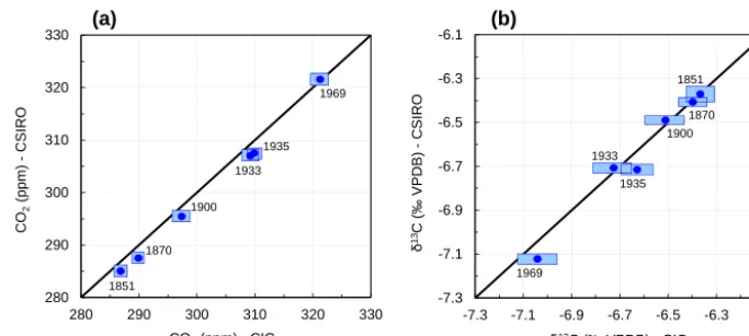
To demonstrate the system performance and reproducibil-ity, we analysed six ice samples of the recent past (1851– 1969 AD) from Law Dome, Antarctica (DE08, 66◦430S, 113◦120E). This was done in a comparison study with CSIRO. The range of sample ages allowed for a compari-son across a relatively wide range of CO2andδ13C values.
These samples were also part of an independent study pub-lished earlier (Rubino et al., 2013). Note that DE08 was
dry-drilled and therefore the difference in the measurement sys-tems that addresses drilling fluid contamination (i.e. separa-tion by GC in the CIC system) is not tested. We measured replicates (n=2 to 4) on the egg-shaped pieces remaining after the samples have been processed at CSIRO using their cheese grater dry extraction system. To allow a realistic as-sessment of measurement reproducibility, the replicates were measured on different days. The pooled standard deviation, used as a measure to estimate the overall analytical preci-sion of our system for single measurements, was 2.0 ppm and 0.11 ‰ for CO2andδ13C, respectively (n=18). Compared
with the results from CSIRO, good agreement within the as-signed 1σ uncertainties was found for both CO2 andδ13C
(Fig. 7). While the agreement betweenδ13C results is high (average CIC – CSIRO=0.02 ‰), a small systematic offset of +1.8 ppm seems to exist for CO2. An obvious