www.the-cryosphere.net/8/417/2014/ doi:10.5194/tc-8-417-2014
© Author(s) 2014. CC Attribution 3.0 License.
The Cryosphere
Implementation and evaluation of prognostic representations of the
optical diameter of snow in the SURFEX/ISBA-Crocus detailed
snowpack model
C. M. Carmagnola1, S. Morin1, M. Lafaysse1, F. Domine2, B. Lesaffre1, Y. Lejeune1, G. Picard3, and L. Arnaud3 1Météo France – CNRS, CNRM – GAME UMR3589, Centre d’Études de la Neige, Grenoble, France
2Takuvik Joint International Laboratory, CNRS and Université Laval, Québec (QC), Canada 3CNRS, UJF Grenoble, LGGE, Grenoble, France
Correspondence to: C. M. Carmagnola ([email protected])
Received: 22 July 2013 – Published in The Cryosphere Discuss.: 6 September 2013 Revised: 18 December 2013 – Accepted: 4 February 2014 – Published: 17 March 2014
Abstract. In the SURFEX/ISBA-Crocus multi-layer snow-pack model, the snow microstructure has up to now been characterised by the grain size and by semi-empirical shape variables which cannot be measured easily in the field or linked to other relevant snow properties. In this work we in-troduce a new formulation of snow metamorphism directly based on equations describing the rate of change of the op-tical diameter (dopt). This variable is considered here to be equal to the equivalent sphere optical diameter, which is in-versely proportional to the specific surface area (SSA).dopt thus represents quantitatively some of the geometric charac-teristics of a porous medium. Different prognostic rate equa-tions ofdopt, including a re-formulation of the original Cro-cus scheme and the parameterisations from Taillandier et al. (2007) and Flanner and Zender (2006), were evaluated by comparing their predictions to field measurements carried out at Summit Camp (Greenland) in May and June 2011 and at Col de Porte (French Alps) during the 2009/10 and 2011/12 winter seasons. We focused especially on results in terms of SSA. In addition, we tested the impact of the dif-ferent formulations on the simulated density profile, the to-tal snow height, the snow water equivalent (SWE) and the surface albedo. Results indicate that all formulations per-form well, with median values of the RMSD between mea-sured and simulated SSA lower than 10 m2kg−1. Incorporat-ing the optical diameter as a fully fledged prognostic variable is an important step forward in the quantitative description of the snow microstructure within snowpack models, because it
opens the way to data assimilation of various electromagnetic observations.
1 Introduction
Snow is a dynamic medium that undergoes continuous ther-modynamical and mechanical processes leading to changes in its microstructure (Colbeck, 1983; Dominé and Shepson, 2002; Flin et al., 2004; Schneebeli and Sokratov, 2004). A good representation of this so-called “snow metamor-phism” within snowpack models is crucial, since the snow microstructure has a significant impact on many macroscopic properties of the snowpack itself. For instance, optical prop-erties such as the transmission of light trough the snow-pack or the surface albedo and chemical exchanges between air and snow are strongly affected by the snow microstruc-ture (Warren, 1982; Meirold-Mautner and Lehning, 2004; Domine et al., 2008). Therefore, designing snow physical models in such a way that they can accurately simulate the metamorphic processes can improve the calculation of the energy and mass budget of snow-covered surfaces (Flanner and Zender, 2006; Taillandier et al., 2007), avalanche fore-casting (Brun et al., 1989, 1992; Durand et al., 1999) and the modelling of climate and of air–snow exchanges of reactive chemical species (Barret et al., 2011).
temperature, density and liquid water content (Essery et al., 2013). More detailed models, in order to simulate snow ag-ing and albedo evolution, include a representation of grain size growth. In the Community Land Model (CLM, Oleson et al., 2010), for instance, dry snow aging is represented as an evolution of the ice effective grain size, which evolves following the microphysical model described by Flanner and Zender (2006). More complex models also incorporate a no-tion of grain shape (Brun et al., 1989, 1992; Lehning et al., 2002). This notion can be important if the aim is to predict an estimate of the avalanche hazard (Durand et al., 1999). In the SURFEX/ISBA-Crocus (Crocus hereinafter) multi-layer snow model (Brun et al., 1989, 1992; Vionnet et al., 2012), metamorphism is currently represented by equations describ-ing the evolution of the snow grain size, the dendricity and the sphericity. These variables, however, are semi-empirical and can neither be measured easily in the field nor directly linked to other relevant snow properties. In addition, this representation makes data assimilation efforts operating on physical properties of snow particularly cumbersome (Toure et al., 2011; Dumont et al., 2012a).
Among scalar variables describing the microstructure of snow and which can be derived from the 3-D geometry of this porous medium (Flin et al., 2003; Löwe et al., 2011), the spe-cific surface area (SSA) has gained increased attention over the past decade. SSA is defined as the total area at the ice/air interface in a given snow sample per unit mass. This variable is impacted by snow aging in a potentially predictable way (Flin et al., 2004; Legagneux and Dominé, 2005; Flanner and Zender, 2006) and generally decreases over time, with values ranging from 224 m2kg−1for diamond dust crystals (Domine et al., 2012) to less than 2 m2kg−1for melt-freeze crusts (Domine et al., 2007). Moreover, SSA is a practical metric for relating the microphysical state of the snowpack to snow electromagnetic characteristics, such as snow albedo and penetration depth (Wiscombe and Warren, 1980; Flan-ner and Zender, 2006) and microwave behaviour (Brucker et al., 2011; Roy et al., 2013a). A rich data set of SSA measurements is now available, since SSA can be retrieved from remote sensing (Kokhanovsky and Schreier, 2009; Du-mont et al., 2012b; Mary et al., 2013), computed by micro-tomography under both isothermal (Flin et al., 2004; Löwe et al., 2011; Schleef and Loewe, 2013) and temperature gra-dient conditions (Schneebeli and Sokratov, 2004; Calonne et al., 2014; Riche et al., 2013) and measured in the field using optical methods (Matzl and Schneebeli, 2006; Gallet et al., 2009; Arnaud et al., 2011).
SSA is inversely proportional to the equivalent spheres’ diameter, which is the diameter of a monodisperse collection of disconnected spheres featuring the same surface area/mass ratio. The equivalent spheres’ diameter is often used inter-changeably with the snow optical diameter (dopt). This allows
for writing
SSA= 6
dopt×ρice
, (1)
whereρice is the density of ice (917 kg m−3). Unlike grain size, a quantity with an ambiguous definition and for which it is difficult to obtain accurate values from visual inspections (Fily et al., 1997; Grenfell and Warren, 1999; Fierz et al., 2009),doptis a well-defined variable representing some ge-ometric characteristics of a porous medium (Giddings and LaChapelle, 1961; Warren, 1982; Grenfell et al., 1994). If the purpose is to model air–snow exchanges of chemical species, it is more convenient to use SSA, whereasdoptis more ade-quate for describing snow optical properties. In the following we will present results in terms of bothdoptand, alternatively, SSA.
were used at Summit Camp (Greenland) in May and June 2011 and during the 2009/2010 and 2011/2012 winter sea-sons at Col de Porte (French Alps). During these field cam-paigns, SSA data were acquired with high vertical resolution (about 1 cm), allowing for testing of the accuracy of the dif-ferent representations of dry metamorphism.
2 Metamorphism in SURFEX/ISBA-Crocus
2.1 Model overview
SURFEX (Surface Externalisée, Masson et al., 2013) is the surface modelling platform developed by Météo-France. It has been designed to be coupled with atmospheric and hydro-logical models and contains independent physical schemes like ISBA for natural land surface, TEB (Town Energy Bal-ance model) for urbanised areas and FLake for lakes. ISBA (Interaction Sol-Biosphère-Atmosphère) includes, in turn, several sub-modules simulating the exchanges of energy and water between the soil–vegetation–snow continuum and the atmosphere above. For snow, different scheme options are available within ISBA, the most detailed of them being Cro-cus (Brun et al., 1989, 1992; Vionnet et al., 2012).
Crocus is a unidimensional model able to compute the en-ergy and mass balance of the snowpack. To this end, the ver-tical profile of the physical properties of snow is represented by a large number of numerical layers (Vionnet et al., 2012). The model includes a detailed description of the time evolu-tion of the snow microstructure. To implement the metamor-phism laws, a semi-quantitative formalism describing snow as a function of continuous parameters has been introduced into Crocus (Brun et al., 1992). These parameters are the dendricityδ (dimensionless, varying between 0 and 1), the sphericitys (dimensionless, also varying between 0 and 1) and the grain sizegs (corresponding to the diameter of the grain, in m). Two main classes of snow types are consid-ered by Crocus. Initialδ ands values are prescribed to ev-ery freshly fallen snow layer, depending on wind speed and temperature. In the case of low wind and cold temperature conditions,δandsare set to 1 and 0.5, respectively. A layer is considered dendritic as long as precipitated snow crystals are still recognisable. Whenδ, which always decreases with snow aging, reaches 0, snow enters the non-dendritic state and the variables describing its microstructure are switched tos andgs (Vionnet et al., 2012; Morin et al., 2013). The time evolution of dendricity, sphericity and grain size fol-lows empirical laws whose parameters were adjusted through experimental investigations. In the case of dry snow, these laws depend mostly on temperatureT and temperature gra-dientG (Brun et al., 1989, 1992; Vionnet et al., 2012). In particular, three regimes are distinguished: weak tempera-ture gradient (G≤5 K m−1), middle temperature gradient (5 K m−1< G≤15 K m−1) and strong temperature gradient (G >15 K m−1). In the latter case,gsincreases over time
fol-lowing the parameterisation described by Marbouty (1980). For wet snow metamorphism, evolution laws only depend on liquid water content (Brun, 1989).
2.2 Impact of the snow microstructure within the model
The snow microstructural variables (δ,s andgs) are com-puted for every time step and for each layer within the meta-morphism routine of Crocus. Other processes, however, can modify these variables. In addition, the microstructural prop-erties are used in turn to calculate different physical quanti-ties. In this section we describe briefly where and how, apart from the metamorphism routine, the microstructural vari-ables are used or modified within the model.
2.2.1 Snow compaction
Snow layer settling due to the combined effect of the meta-morphism and the weight of the overlaying layers is com-puted using a Newtonian viscosity law, which leaves the mass of each layer unchanged and reduces the layer thickness in proportion to density increase. Snow viscosity depends on snow density, temperature and liquid water content, but also on microstructural properties (depth hoar, for instance, has a lower compaction rate).
2.2.2 Snow surface albedo and solar radiation transmission through the snowpack
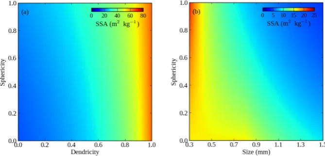
Fig. 1: Relationship between SSA and grain variables in the original Crocus version. Empirical
equations (Vionnet et al., 2012) were used to estimate the optical diameter (a) from dendricity and
sphericity in the dendritic case and (b) from sphericity and size in the non-dendritic case. Then, the
optical diameter was converted into SSA using Eq. 1.
29
Fig. 1. Relationship between SSA and grain variables in the original Crocus version. Empirical equations (Vionnet et al., 2012) were used to estimate the optical diameter (a) from dendricity and sphericity in the dendritic case and (b) from sphericity and size in the non-dendritic case. Then, the optical diameter was converted into SSA using Eq. (1).
2.2.3 Snowfall and grid resizing
Crocus can modify the discretisation of the vertical grid, in order to keep the number of layers below a predetermined value (typically 50). When a new snowfall layer is added to an existing snowpack, the model first prescribes specific values accounting for its microstructure. Then, if the freshly fallen snow layer and the existing top layer have similar char-acteristics, they are merged. The similarity between both lay-ers is determined from the value of the sum of their differ-ences in terms ofδ,sandgs, each weighted with an appro-priate coefficient ranging from 0 to 200: 0 corresponds to the case in which the same snow type is present in both layers and 200 to very different snow types. In other words, merg-ing is only possible for layers which are similar enough in terms of snow types. If a new numerical snow layer is built from two older layers, its characteristics are calculated in or-der to conserve the averaged weighted optical diameter of the former layers. This ensures a strong consistency in the evolu-tion of surface albedo. When, instead, merging is not possi-ble, a new numerical layer is added to the existing snowpack. A complete description of the grid resizing in Crocus can be found in Vionnet et al. (2012).
2.2.4 Wind drifting
Snow compaction and metamorphism due to wind drift are taken into account by Crocus (Brun et al., 1997; Guyomarc’h and Merindol, 1998; Vionnet et al., 2013). The impact of wind on surface layer properties is evaluated in three steps. First, a mobility index is calculated for each layer from its snow type and density. This index, which describes the po-tential for snow transport, is highest for fresh snow and tends to decrease with sintering and compaction. Mobility is then combined with wind speed to compute a driftability index. Finally, density and snow types are modified in the case of
transport: in each layer, δ and gs are reduced ands is in-creased according to the driftability index.
2.3 Time evolution of the optical diameter within the model
In Sect. 2.1 we have presented the original Crocus formula-tion of snow metamorphism laws, as developed by Brun et al. (1992). That formulation describing snow grains by their dendricity, sphericity and size and treating the optical diam-eter as a diagnostic variable of the model is called B92 here-inafter. Here we introduce a new formulation (called C13) in which the original evolution laws are re-formulated in terms ofdoptands. Indeed, both dendricity and grain size, plotted as a function of time, are monotonic functions, the former always decreasing when snow is in a dendritic state and the latter always increasing in a non-dendritic state. Thus, it is possible to replaceδandgs by a single variable, the optical diameter, which is always increasing with time and whose rate of change can be easily deduced from the same equations as B92.doptis then turned into a prognostic variable of the model. However, since this variable alone is not sufficient to describe uniquely the snow microstructure, in C13 sphericity still remains, in order to take into account the shape of the crystals (rounding and facets).
2.3.1 Formulation C13
In formulation C13, all original equations of B92 including
δ,sandgswere re-written in terms ofdoptands. In practice, δandgswere replaced by expressions that are functions of onlydoptands. Based on the original relationships linking δ,s andgs todoptdescribed in Sect. 2.2.2, we replaced the dendricity by
δ=
dopt
α −4+s
s−3 (2)
and the grain size by
gs=α (4−s) , (3)
where dopt and gs are expressed in m and α is equal to 10−4m. Sinceδ andsvary between 0 and 1, Eq. (2) estab-lishes thatdoptvalues for dendritic snow range from 0.1 mm, corresponding to an SSA value of 65 m2kg−1, to 0.4 mm, corresponding to an SSA of 16 m2kg−1 (see Fig. 1). The transition from a dendritic to a non-dendritic regime, which occurs whenδ reaches 0 in B92, was also re-formulated in terms ofdoptands:
dopt< α (4−s) dendritic case (4a)
dopt≥α (4−s) non-dendritic case (4b) Thus, snow enters its non-dendritic state ifdoptgrows beyond a certain threshold. The higher the sphericity value, the easier it will be fordoptto exceed this threshold.
The snow optical diameter was introduced in all Crocus routines described in Sect. 2.2. In most cases, this leads to a significant simplification of the equations. For example, using the optical diameter as a prognostic variable allows for computing of the snow albedo directly, which depends explicitly ondopt, and the microstructural characteristics of merged layers, which are calculated in order to conserve the averaged weighteddoptof the former layers. Elsewhere, the change of variable is not as trivial. This is the case, for in-stance, for wind drifting. When a new fresh snow layer is created, its optical diameter is set by default to 10−4m. This value corresponds to the combination ofd=1 ands=0.5 in B92, as can easily be seen using Eq. (2). In the case of wind drifting, however, the dopt value is modified depend-ing on the wind speed. Therefore, the evolution rates of the snow microstructural properties caused by the snow drifting (reported in Table 3 of Vionnet et al. (2012) in their B92 for-mulation) here have to be re-written for the optical diameter as follows:
∂dopt ∂t =α
δ
2τ(s−3)+
1−s τ (δ−1)
dendritic case (5a)
∂dopt
∂t = −2αs
1−s
τ non-dendritic case (5b)
wheret is time expressed in hours,τ is computed from the driftability index (which depends on the wind speed and the microstructural properties of snow, see Sect. 2.2.4) and rep-resents the time characteristic for snow grain changes under wind transport, andδ can be derived through Eq. (2). In the case of no drifting,τ tends to infinity and Eq. (5) leads to unchanged values fordopt(Brun et al., 1992, 1997; Vionnet et al., 2012).
The most significant differences between C13 and B92 concern the re-formulation of the dry metamorphism laws. Combining the original Crocus rate equations for the snow microphysical variables (reported in Table 1 of Vionnet et al., 2012) and Eqs. (2–4), we obtained new parametric laws de-scribing the rate of change ofdopt. These equations are re-ported in Table 2 along with the rate equations fors, which are identical to those of B92. The rate of change ofdopt (al-ways increasing) ands(either increasing or decreasing) are a function of the vertical temperature gradient (G, in K m−1), the temperature (T, in K) and the time (t, in days). Six cases are distinguished, depending on theGvalue (weak, middle and strong temperature gradient) and the regime (dendritic and non-dendritic snow). When G >15 K m−1 ands=0,
doptof non-dendritic snow increases over time following the parameterisation of Marbouty (1980), which allows for pre-dicting of depth hoar growth rate. In the original B92 formu-lation, non-dendriticdoptbecame a function ofgsonly when the latter exceeded an empirical threshold set to 8·10−4m. In C13 we do not have any information aboutgsand there-fore we have removed this threshold. This means that in the case of a strong temperature gradient metamorphism, C13 will lead todoptvalues higher than those of B92. Aside from that difference, formulations C13 and B92 are supposed to give the same results (see Sect. 2.3.4), as C13 consists in a reformulation, in terms of optical diameter, of the original metamorphism laws of B92 expressed in terms of dendricity and snow grain size.
2.3.2 Formulation T07
Taillandier et al. (2007) performed several experiments dur-ing which the SSA was measured under isothermal and tem-perature gradient conditions. Based on this data set, they pro-posed a parameterisation of the rate of decay of SSA (formu-lation T07), whose implementation in Crocus is described in this section.
The SSA decrease over time under isothermal (ET) and temperature gradient (TG) conditions can be written as SSAET(t )=AET(SSA0, T )−BET(SSA0, T )
·ln
t+e
CET(SSA0,T ) BET(SSA0,T )
(6a) SSATG(t )=ATG(SSA0, T )−BTG(SSA0, T )
·ln
t+e
CTG(SSA0,T ) BTG(SSA0,T )
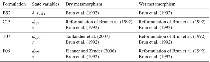
Table 1. Metamorphism formulations implemented in Crocus. B92 (Brun et al., 1992) describes snow grains in terms of dendricity (δ), sphericity (s) and size (gs). C13 (this work), T07 (Taillandier et al., 2007) and F06 (Flanner and Zender, 2006) use optical diameter (dopt) ands. See text for more details.
Formulation State variables Dry metamorphism Wet metamorphism
B92 δ,s,gs Brun et al. (1992) Brun et al. (1992)
C13 dopt Reformulation of Brun et al. (1992) Reformulation of Brun et al. (1992)
s Brun et al. (1992) Brun et al. (1992)
T07 dopt Taillandier et al. (2007) Reformulation of Brun et al. (1992)
s Brun et al. (1992) Brun et al. (1992)
F06 dopt Flanner and Zender (2006) Reformulation of Brun et al. (1992)
s Brun et al. (1992) Brun et al. (1992)
Table 2. Metamorphism laws for formulation C13 in the case of dry snow.Gis the vertical temperature gradient (∇T = |∂T /∂z|, in K m−1), T the temperature (in K) andtthe time expressed in days.f,g,hand8are empirical functions to predict depth hoar growth rate in the case of highGvalues (Marbouty, 1980; Vionnet et al., 2012).αis equal to 10−4m.
∇T Non-dendritic snow Dendritic snow
G≤5 K m−1
∂dopt
∂t = −2αs∂s∂t
∂dopt
∂t =α "
−2×108×10−6000/T(s−3)+∂s
∂t
dopt α −1
s−3
#
∂s
∂t =109×10−6000/T ∂s∂t=109×10−6000/T
5< G≤15 K m−1
∂dopt
∂t = −2αs∂s∂t ∂dopt
∂t =α "
−2×108×10−6000/TG0.4(s−3)+∂s ∂t
dopt α −1
s−3
#
∂s
∂t = −2×108×10
−6000/TG0.4
G >15 K m−1 ifs >0:
∂dopt
∂t = −2αs∂s∂t and∂s∂t = −2×108×10
−6000/TG0.4
∂s
∂t= −2·108×10
−6000/TG0.4 ifs=0:∂dopt
∂t =12f (T )h(ρ)g(G)8and∂s∂t =0
whereA,B andC are fitted coefficients that depend on the actual temperature of the layer (T) and its initial snow SSA (SSA0). No density effect is predicted by those equations, since experiments performed by Taillandier et al. (2007) failed to detect a significant influence of that variable. For SSA0, in order to be consistent with the maximum SSA value allowed by formulation B92, we used:
SSA0=
6
ρice·10−4m
(7)
Equation (6a and b) can be merged, using a hyperbolic tan-gent form, into a single equation where SSA evolution de-pends continuously on temperature gradient. For this aim we defined two new coefficients as follows:
DTG(∇T )=0.5+0.5·tanh [0.5·(∇T−10)] (8a)
DET(∇T )=1−DTG(∇T ) (8b)
This allowed a unified equation to be written which formu-lates SSA as a function of the temperature gradient and the temperature:
SSA(t )=DTG(∇T )·SSATG(t )+DET(∇T )·SSAET(t ) (9)
Equation (9) computes SSA using Eq. (6a) when ∇T <
5 K m−1and Eq. (6b) when∇T >15 K m−1. When the tem-perature gradient is between these two values, a weighted average of SSAETand SSATGis used. From Eq. (9), with a second-order Taylor series development we can finally obtain the SSA decay:
SSA(t+1t )=SSA(t )+∂SSA(t )
∂t 1t+
1 2
∂2SSA(t ) ∂t2 1t
2 (10)
Table 3. Overview of the measurements acquired at Summit Camp in 2011 and at Col de Porte during the winters of 2009/2010 and 2011/2012. These data were used to evaluate the different representations of the snow optical diameter growth rate implemented in SURFEX/ISBA-Crocus.
Field campaigns Measurements of snow properties
Site Period Variable (unit) Instrument Instrument Time resolution
accuracy
Summit Camp,
05/05/2011–25/06/2011 Density (kg m
−3) Steel sampler
10 % ∼daily (32 vertical profiles)
Greenland (3210 m a.s.l.) SSA (m2kg−1) DUFISSS
06/01/2010–14/04/2010 Density (kg m
−3) Steel sampler
10 % ∼weekly (14 vertical profiles)
Col de Porte, SSA (m2kg−1) DUFISSS
French Alps (1325 m a.s.l.)
21/12/2011–28/03/2012 Density (kg m
−3) Steel sampler
10 % ∼weekly (16 vertical profiles)
SSA (m2kg−1) ASSSAP
Fig. 2: Time evolution of layer age (a) and SSA (b) in a multi-layer model, simulated using the
parametrization T07 (Taillandier et al., 2007). Layer 1 and layer 2 are created at different times to
take into account new snowfalls. Att= 30 days, these two layers aggregate and give rise to layer 3.
The age of the new-formed layer has to be chosen arbitrarily and this has an impact on the SSA rate
of change.
30
Fig. 2. Time evolution of layer age (a) and SSA (b) in a multi-layer model, simulated using parameterisation T07 (Taillandier et al., 2007). Layer 1 and layer 2 are created at different times to take into account new snowfalls. Att=30 days, these two layers aggregate and give rise to layer 3. The age of the newly formed layer has to be chosen arbitrarily and this has an impact on the SSA rate of change.
LAnd Surface Scheme), in which Roy et al. (2013b) have already implemented parameterisation T07 successfully. In multi-layer snow models, however, when two or more layers merge the age of the new-formed layer has to be chosen arbi-trarily. For instance, we can decide to keep the age of either the younger or the older of the former layers, or a mean of them. All choices may be equally valid and lead to different SSA rates of change (Fig. 2). In our simulations, we com-puted the age of the new layer by making a weighted average of the ages of the former layers. The weight chosen was the same as that used to compute the new optical diameter (see Sect. 2.2.3).
Formulation T07 uses a logarithmic function to fit the de-creasing trend of SSA. Legagneux et al. (2004) showed that this approach leads to a good approximation of a more gen-eral evolution law of SSA that can be easily derived from
grain coarsening theories. This approximation, however, only applies for times less than 150 days and predicts that the SSA will become negative after about a year (Taillandier et al., 2007). For this reason, in order to avoid unrealistic values, in our simulations the minimum SSA was forced to 8 m2kg−1. This allows the parametric laws of T07 to be adequate for most applications to seasonal snowpacks, in which SSA do not go, in general, below that value (Taillandier et al., 2007). In contrast, formulation T07 was not designed to simulate the decreasing trend of SSA over time periods longer than a few months. In light of these considerations, we decided to eval-uate this formulation only on the seasonal snowpack at Col de Porte and not on the permanent snowpack at Summit. 2.3.3 Formulation F06
Flanner and Zender (2006) developed a model (referred to as F06 here) able to simulate diffusive vapour flux amongst collections of disconnected ice spheres of different radii. In this model, limited to dry snow, the optical diameter can be computed for any combination of snow density, temperature, temperature gradient and initial size distribution. A paramet-ric equation, which fits model output and is computationally inexpensive, was included in the Community Land Model by Oleson et al. (CLM, 2010). Here we followed the same ap-proach by incorporating this equation into Crocus.
The optical diameter was computed as follows:
dopt(t+1t )=dopt(t )+2· dr
dt ·1t (11)
where: dr
dt =
dr
dt 0
·
τ (r−r0)+τ
1κ
(12)
r is the optical radius (in µm), r0 is the initial optical ra-dius for fresh snow (in µm) and t is time (in hours). The initial rate of change of optical radius ddrt
(Flanner and Zender, 2006). The domain covered by these tables includes densities ranging from 50 to 400 kg m−3, tem-peratures ranging from 223.15 to 273.15 K and temperature gradients ranging from 0 to 300 K m−1. The initial SSA can be set to 60, 80 or 100 m2kg−1. In order to be consistent with the maximum SSA value allowed by formulation B92, we chose an initial SSA of 60 m2kg−1, which corresponds tor0= 50 µm in Eq. (12).
2.3.4 Comparison of the different formulations
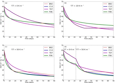
The SSA rates of decay predicted by the above-described formulations are shown in Fig. 3. All curves were plotted for a constant temperature of−20◦C and a constant density of 200 kg m−3. Different temperature gradient values ranging from 0 to 50 K m−1were tested; in the lower right panel,∇T was set to 0 K m−1untilt=22.5 days and to 50 K m−1 there-after. In order to have a similar initial SSA for all schemes, about 60 m2kg−1, B92 was initialised with d=0.964 and
s=0.5 and C13 with dopt=109 µm and s=0.5. Regard-less of the formulation chosen, the most rapid snow ag-ing is always produced by the combination of low density, high temperature and large temperature gradient. However, on closer inspection the comparison of the four metamor-phism formulations shows some differences. B92 and C13, for instance, display a discontinuous derivative when snow enters the non-dendritic state. This discontinuity, which has no physical meaning and comes from the empirical param-eterisation of the rate equations, is not present in T07 and F06. Indeed, in terms of SSA rate of change there is no distinction for T07 and F06 between the dendritic and non-dendritic regimes; this distinction remains true only for the time evolution of sphericity, which is identical to that of B92 for all formulations. In addition, it is easy to see that B92 and C13 differ only when∇T is high (>15 K m−1). In this case, in the C13 formulation SSA starts decreasing following the parametrization of Marbouty (1980) as soon as the non-dendritic state is reached; B92, instead, makes SSA decrease only whengs>8·10−4m.
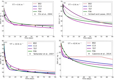
In Fig. 4, the formulations of the SSA rate of change were compared to cold room measurements. Flin et al. (2004) computed snow SSA from micro-tomography during an isothermal experiment atT=−2◦C; Schleef and Loewe (2013) analysed micro-tomographic images acquired dur-ing an isothermal experiment at T = −20◦C; Taillandier et al. (2007) determined SSA by measuring the adsorp-tion of methane at 77 K on snow that had evolved un-der temperature gradient conditions (Tmean= −10◦C,∇T = 33 K m−1); Calonne et al. (2014) used micro-tomographic images to compute SSA under temperature gradient condi-tions (Tmean= −4◦C,∇T =43 K m−1). Results reveal that, albeit with some differences, all formulations perform sim-ilarly. Formulation F06 reproduces the experimental data slightly better than the other formulations, whereas B92 and C13 generally perform not quite as well, mostly because of
their change in regime between dendritic and non-dendritic snow, which does not match the observed behaviour of SSA decrease. Analogous results are expected to be found when these different representations of the SSA rate of change are implemented directly in Crocus.
3 Materials and methods
In this section we describe the sites where measurements were carried out, the meteorological forcing data used to run the simulations, the snow data set acquired to evaluate the accuracy of the metamorphism formulations, the model runs and the statistical metrics used to compare Crocus outputs to observations.
3.1 Experimental sites
3.1.1 Summit Camp
A two-month field campaign took place in May and June 2011 at Summit Camp (72◦360N, 38◦250W). This research station is located at the peak of the Greenlandic ice cap, at 3210 m a.s.l. (http://www.summitcamp.org/). In this area, snowfall can occur in all seasons (Albert and Hawley, 2000) and the accumulation rate is not seasonally uniform. Wind conditions can change dramatically during the year (Albert and Shultz, 2002) and have a strong impact on snow sur-face layers. During our campaign, the air temperature was always negative and no liquid water was ever found within the snowpack. Several wind drifting events occurred, with wind speeds up to 15 m s−1.
3.1.2 Col de Porte
Fig. 3: Time evolution of snow SSA, according to different metamorphism formulations. B92 stands
for Brun et al. (1992), T07 for Taillandier et al. (2007) and F06 for Flanner and Zender (2006),
whereas C13 refers to this work. Temperature was set to -20◦C and density to 200 kg m−3. The four
panels correspond to different temperature gradient values.
31
Fig. 3. Time evolution of snow SSA, according to different metamorphism formulations. B92 stands for Brun et al. (1992), T07 for Taillandier et al. (2007) and F06 for Flanner and Zender (2006), whereas C13 refers to this work. Temperature was set to−20◦C and density to 200 kg m−3. The four panels correspond to different temperature gradient values.
3.2 Meteorological data
In order to run SURFEX/ISBA-Crocus simulations, a com-plete meteorological forcing has to be provided to the model. In its basic configuration, Crocus requires the following driv-ing variables: air temperature and specific humidity at 2 m above ground, wind speed at 10 m above ground, snowfall and rainfall rates and incoming short-wave and long-wave radiations.
For simulations at Summit, input variables were provided by the ERA-Interim reanalysis (Dee et al., 2011) with a 3 h time step. This data set extends back to 1979 and has a spa-tial resolution of about 80 km, with 60 vertical levels up to 0.1 hPa (about 64 km). Since meteorological conditions over the upper Greenlandic ice cap are quite homogeneous, we used the 80 km grid cell nearest to the Summit Camp lo-cation, without downscaling the data to a smaller numerical grid. For the period of our field campaign, ERA-Interim data were replaced by in situ measurements acquired on an hourly basis by the Summit Automatic Weather Station (AWS, Stef-fen et al., 1996). Air temperature and relative humidity were measured using a Type-E thermocouple (estimated accuracy of 0.1◦C) and a Campbell Sci. CS-500 (accuracy of 10 %), respectively. Wind speed was recorded with a RM Young propeller-type vane (estimated accuracy of 0.1 m s−1) and
short-wave incoming radiation was measured using a Li Cor photodiode (nominal accuracy of 15 %). No measurement of precipitation rates and incoming long-wave radiation were performed by AWS. Figure S1 shows a comparison between AWS measurements and ERA-Interim reanalysis for four dif-ferent variables during the period April–July 2011.
Fig. 4: Comparison between the SSA rate of decay predicted by different metamorphism
formula-tions and measured during cold room experiments. The isothermal experiments of Flin et al. (2004)
and Schleef and Loewe (2013) were performed atT = -2◦C andT = -20◦C, respectively. In the
temperature gradient experiment of Taillandier et al. (2007),∇Twas 33 K m−1and the temperature
was -10◦C. These values were respectively 43 K m−1and -4◦C for the temperature gradient
ex-periment of Calonne et al. (in prep.). In (b), we plotted both the data (black dots) and the fit (black
dotted line) according to Eq. 7 of Schleef and Loewe (2013).
32
Fig. 4. Comparison between the SSA rate of decay predicted by different metamorphism formulations and measured during cold room experiments. The isothermal experiments of Flin et al. (2004) and Schleef and Loewe (2013) were performed atT= −2◦C andT= −20◦C, respectively. In the temperature gradient experiment of Taillandier et al. (2007),∇T was 33 K m−1and the temperature was−10◦C. These values were respectively 43 K m−1and−4◦C for the temperature gradient experiment of Calonne et al. (2014). In (b), we plotted both the data (black dots) and the fit (black dotted line) according to Eq. (7) of Schleef and Loewe (2013).
3.3 Snow data
Measurements of several snow properties were performed at Summit Camp and Col de Porte in order to evaluate the dif-ferent representations of the optical diameter of snow imple-mented in SURFEX/ISBA-Crocus (see Table 3).
At Summit, density was measured every day, down to about 80 cm and with a vertical resolution better than 4 cm, by sampling the snow with a 250 cm3rectangular steel cutter (Fierz et al., 2009; Conger and McClung, 2009). At the same time, snow specific surface area measurements were per-formed using DUFISSS (DUal Frequency Integrating Sphere for Snow SSA measurement, Gallet et al., 2009), an integrat-ing sphere which allows for retrievintegrat-ing of SSA from infrared reflectance measurements. In the top 10 cm we kept a verti-cal resolution of 1 cm, whereas below that depth and down to about 80 cm a 2 to 4 cm resolution was used. The snow height was monitored by the AWS, using a Campbell SR-50 with 1 mm precision. A more in-depth description of the snow data set acquired at Summit can be found in Carmag-nola et al. (2013).
At Col de Porte, 14 and 16 vertical profiles of density and SSA were acquired during the winter of 2009/2010 and 2011/2012, respectively. Density was recorded for each snow
the solar zenith angle, are currently not represented in Cro-cus.
3.4 Model runs
At Summit, the simulations were run from 1 February 1979 to 1 July 2012. The output time step was set to 6 h and the to-tal initial snow height was set to 10 m. The snowpack was ini-tialised with eight layers, prescribing thinner and less dense layers near the surface. The choice of the profile used to ini-tialise the simulations has a very small impact on the final results of the model more than 30 yr later. The impact of re-placing ERA-Interim forcing data by in situ measurements during our field campaign period is also negligible.
At Col de Porte, the simulations were run from 1 Au-gust 1993 to 31 September 2012, with an output time step of 6 h. We used, for the whole time period, the same initiali-sation procedure, consisting of assigning to all ground layers the mean annual temperature at Col de Porte. This proce-dure ensures that the temperature data of the simulated up-permost ground layers attain reasonable equilibrium with en-vironmental conditions after 16 and 18 yr of simulation (for the 2009–2010 and 2011–2012 snow seasons, respectively). 3.5 Definitions of metrics
In order to evaluate the agreement between observations and simulations, we define the quantity1SSA, which represents the root mean square deviation (RMSD) between measured and simulated SSA for a given date:
1SSA= s
P
h SSAobs,h−SSAsim,h2 Nh
(13) where SSAobs,h and SSAsim,h are the measured and
simu-lated SSA, respectively, andNh is the total number of
con-sidered SSA values for a given vertical profile. In prac-tice, to compute1SSA both measurements and simulations were interpolated on a 1 mm vertical grid and the difference SSAobs,h−SSAsim,hwas calculated for every SSAobs,hvalue.
The same quantity can be expressed in terms ofdopt. Ev-ery single measured and simulated SSA value was then con-verted into respectively doptobs,h and doptsim,h, in order to compute the RMSD for the optical diameter:
1dopt =
v u u t
P h
doptobs,h−doptsim,h2 Nh
(14)
4 Results
4.1 Field measurements
At Summit, the upper metre of the snowpack was dominated by faceting rounded grains with density values ranging from
280 to 350 kg m−3, interspersed with hard wind slabs with densities up to 400 kg m−3. At the surface, in the case of fresh snow precipitation or surface hoar formation, density could be significantly lower (120–140 kg m−3). SSA reached 65–75 m2kg−1 (corresponding to optical diameters of 109 to 93 µm) at the surface when rime, fresh snow or surface hoar were present. For layers deeper than 60 cm, SSA was about 20 m2kg−1(optical diameter of 327 µm). Even if the cold temperatures of the Arctic ice cap make the metamor-phic processes slow, during the campaign we observed a de-crease in SSA over time, along with a slight density inde-crease. Indeed, if we consider the depth between 2 and 15 cm, our first eight vertical profiles (from 5 May to 19 May) have a mean density value of 315±13 kg m−3 and a mean SSA value of 37±3 m2kg−1. These values become, respectively, 335±20 kg m−3and 23±3 m2kg−1for the last eight pro-files (11–25 June). In terms of snow height, results show that during our field campaign, despite frequent small amounts of precipitation, no significant accumulation occurred.
At Col de Porte, density spread over a wide range of val-ues, from 65 kg m−3for fresh snow to 450 kg m−3for melt clusters. In the same way, measured SSA values ranged from 5 m2kg−1(corresponding to an optical diameter of 1.3 mm) for melt-refrozen forms up to 80 m2kg−1 (optical diame-ter of 73 µm) for precipitation particles fallen in weak-wind conditions and at low temperatures. The maximum snow height measured during the 2009/2010 winter season was just above 1 m and the maximum measured SWE was about 300 kg m−2. In 2011/2012, these values were respectively 1.24 m and 390 kg m−2. The daily integrated surface albedo values ranged from 0.95 in the presence of freshly fallen snow to less than 0.5 for dirty and old snow during melting periods.
4.2 Numerical simulations
4.2.1 Summit camp
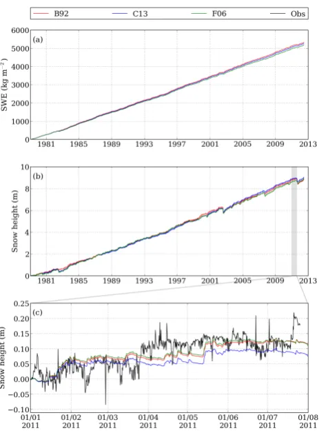
Figure 5 shows the time series of snow height and SWE over the whole simulated period. After about 33 yr of simulations, the different metamorphism formulations (see Sect. 2.3) give similar results, with differences less then 4 % in snow height and less than 3 % in SWE. A comparison with the measured data for the period January–July 2011 (Fig. 5c) shows that the simulated snow height is not always able to capture the observed variability: the general trend is reproduced by the model, but the variations at the daily scale are not. This can be mostly explained by the spatial variability of the snow-pack due to the effect of wind, and in particular to the event-driven deposition of snow, which is frequent in polar regions (Groot Zwaaftink et al., 2013).
Fig. 5: Time evolution of SWE and snow height at Summit. The metamorphism formulations
de-scribed in Sect. 2.3 are represented by different colours: B92 (Brun et al., 1992) in red, C13 (this
work) in blue and F06 (Flanner and Zender, 2006) in green. Observations from AWS are in solid
black. (a) Simulated SWE since 1 February 1979. (b) Simulated snow height since 1 February 1979.
(c) Close up on simulated and measured snow height during our field campaign (all curves are re-set
to zero on 1 January 2011, in order to better compare them).
33
Fig. 5. Time evolution of SWE and snow height at Summit. The metamorphism formulations described in Sect. 2.3 are represented by different colours: B92 (Brun et al., 1992) in red, C13 (this work) in blue and F06 (Flanner and Zender, 2006) in green. Observations from AWS are in solid black. (a) Simulated SWE since 1 February 1979. (b) Simulated snow height since 1 February 1979. (c) Close up on simulated and measured snow height during our field cam-paign (all curves are reset to zero on 1 January 2011, in order to better compare them).
over time within the different layers, which tend to aggregate when their properties become similar. Changing the evolu-tion over time of the optical diameter can in principle have an impact on the simulated density (see Sect. 2.2.1). This im-pact, however, is generally low and all density profiles look similar. In terms of SSA the discrepancies are more impor-tant. In Fig. 7 we show the difference between the SSA pro-files obtained with formulations C13 and F06 and the SSA profile obtained with formulation B92. Since every formu-lation leads to a different snow height and snowpack layer-ing, in order to calculate this difference all SSA profiles were previously interpolated over a 1 mm vertical grid; then, start-ing from the snow surface, SSA values from B92 were sub-tracted from those from C13 and F06 at every 1 mm depth. Results from C13 differ from those from B92 by less than 5 m2kg−1 over the entire profile considered, which is not surprising since C13 is designed after B92. Also, SSA
val-Fig. 6: Simulated density (left column) and SSA (right column) at Summit from 1 April to 31 July
2011. Simulations were run using different metamorphism formulations. From top to bottom: B92
(Brun et al., 1992), C13 (this work) and F06 (Flanner and Zender, 2006).
34
Fig. 6. Simulated density (left column) and SSA (right column) at Summit from 1 April to 31 July 2011. Simulations were run us-ing different metamorphism formulations. From top to bottom: B92 (Brun et al., 1992), C13 (this work) and F06 (Flanner and Zender, 2006).
ues computed with F06 look consistent with those obtained with B92, except for the upper layers. Contrary to the other formulations, in F06 the rate of change of the optical diame-ter also depends on the density and makes light layers evolve more rapidly.
Fig. 7: Comparison in terms of SSA between the metamorphism formulations implemented into
Crocus. In order to compare results obtained using different formulations, all SSA profiles were
interpolated over a 1 mm vertical grid. The plots show the difference between the new formulations
C13 (top) and F06 (bottom) and the original formulation B92, for simulations run at Summit from 1
April to 31 July 2011.
Fig. 7. Comparison in terms of SSA between the metamorphism formulations implemented in Crocus. In order to compare results obtained using different formulations, all SSA profiles were inter-polated over a 1 mm vertical grid. The plots show the difference between the new formulations C13 (top) and F06 (bottom) and the original formulation B92, for simulations run at Summit from 1 April to 31 July 2011.
different simulations are significantly smaller than those be-tween simulations and observations.
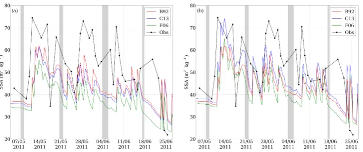
The time evolution of the surface SSA at Summit is pre-sented in Fig. 9. In order to obtain the SSA of the top 1 cm, all simulations were interpolated over a 1 mm vertical grid; then, an exponentially weighted average of the SSA values within the top 1 cm of snow was made (Mary et al., 2013). The general behaviour of the observed SSA is well captured by the simulations. Sometimes, however, the measured SSA in-creased over time, whereas the simulated SSA tended to de-crease. This always occurred in conjunction with strong wind
Fig. 8: Comparison between simulated and measured density (left) and SSA (right) at Summit, on
10 May 2011, 12h00 LT.
36
Fig. 8. Comparison between simulated and measured density (left) and SSA (right) at Summit, on 10 May 2011, 12:00 LT.
events (grey bands represent periods during which the AWS measured wind speed >9 m s−1). These events were only strong enough to reduce the rate of decrease of the simulated SSA but not to make it increase. Observed surface SSA val-ues, on the contrary, show an increase, since measurements were probably performed on wind-drifted snow. Moreover, it is clear that the simulated SSA values underestimate the ob-servations. In the original B92 formulation, indeed, the max-imum allowed SSA value was set to 65 m2kg−1(see Eq. 2). This constitutes a limit for the simulations at Summit, where the surface SSA can easily reach 75 m2kg−1. The new meta-morphism formulations using the optical diameter as a prog-nostic variable allows for reduction of the discrepancies be-tween simulations and observations. In Fig. 9b, for instance, formulations C13 and F06 were run setting the maximum SSA value to 80 m2kg−1and show an improved agreement with the observations. Even in this case, however, the obser-vations are not perfectly reproduced, meaning that our under-standing of the processes involved in the SSA decrease over time is not complete.
4.2.2 Col de Porte
2009/2010 winter season
Figure S2 shows the snow height, SWE and surface broad-band albedo simulated by Crocus over the 2009/2010 winter season. The observed values are reported as well. Model results are generally similar, except during the melting pe-riod, when T07 gives higher height, SWE and albedo values. RMSD between simulations and observations are larger than those between simulations themselves, with values reaching 0.10 m in snow height, 40 kg m−2in SWE and 0.12 in albedo. These results in terms of RMSD are reasonable for this site and consistent with previous studies (Vionnet et al., 2012; Essery et al., 2013; Morin et al., 2013).
The vertical profiles of density and SSA simulated at Col de Porte in 2009/2010 using the four metamorphism formu-lations are presented in Fig. S3. As for Summit, differences
Fig. 9: Time evolution of the SSA of the top 1 cm at Summit. The simulated SSA were obtained
by making a weighted average of the SSA values within the top 1 cm of snow. Grey vertical bands
represent periods of strong wind (wind speed>9 m s−1). Formulations C13 and F06 were run
setting the maximum SSA value to 65 m2kg−1in (a) and to 80 m2kg−1in (b).
37
Fig. 9. Time evolution of the SSA of the top 1 cm at Summit. The simulated SSA were obtained by making a weighted average of the SSA values within the top 1 cm of snow. Grey vertical bands represent periods of strong wind (wind speed>9 m s−1). Formulations C13 and F06 were run setting the maximum SSA value to 65 m2kg−1in (a) and to 80 m2kg−1in (b).
in density are negligible, whereas those in SSA are more sig-nificant. The difference in terms of SSA between results tained with formulations C13, T07 and F06 and results ob-tained with formulation B92 was computed by interpolating all SSA profiles over a 1 cm vertical grid (Fig. S4). Formula-tion C13 gives, as expected, results similar to those obtained with B92, with differences lower than 8 m2kg−1. Right af-ter the snowfall, SSA from T07 are generally lower than the corresponding values from B92; then, within a few days, they become higher (up to 20 m2kg−1) during several weeks and finally match the SSA from B92 after the sharp transition at the beginning of the melt period. It can also be noticed that for the dry and warm conditions that occurred in the middle of March 2010 the surface SSA values obtained using T07 remain larger than the corresponding values simulated using other formulations. This results in higher albedo, which leads in turn to higher snow height and SWE (see Fig. S2). As at Summit, SSA computed with F06 is consistent with that ob-tained with B92, except for the recent upper layers, whose SSA evolves more rapidly using the F06 parameterisation. Regardless of the formulations considered, the smaller dif-ferences are found during the melt period, not only because in this case the SSA values are generally lower, but also be-cause all representations include the same formulation for wet metamorphism (see Table 1).
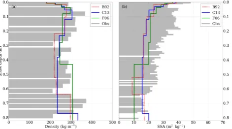
A comparison between simulated and observed density and SSA profiles at Col de Porte on 11 February 2010 is pre-sented in Fig. S5. The total snow height measured that day was 1.04 m, the record for the 2009/2010 winter season. A 1 cm-thick layer of precipitation particles was present at the surface and was sitting on about 35 cm of decomposing and fragmented snow, the rest of the snowpack being made up of melt forms. Even if all formulations underestimate the snow height, the simulated density and SSA values follow the same pattern as the observations. For the density, the simulated val-ues range from 80 kg m−3at the surface to about 350 kg m−3
at the bottom and a quantitative match with the observed val-ues is attained. For the SSA, the range of variations and the vertical layering are not well reproduced.
Figure S6 shows that all formulations perform similarly in terms of snow type and liquid water content. The only significant differences appear when the temperature gradi-ent is between 5 and 15 K m−1. In this case, B92 and C13 make the SSA decrease faster than T07 and F06 in a time pe-riod ranging from about 10 and 60 days since snowfall (see Fig. 3b). This is the main reason why B92 and C13 simulate the presence of faceted crystals between January and Febru-ary, whereas T07 and F06 indicate, for the same period, the presence of decomposing and fragmented snow. Since visual observations between January and February revealed the co-existence, within deep layers, of both faceted and decom-posing crystals, it is not easy to determine which formula-tion matches the observed snow profiles better in terms of snow type. In fact, since the very notion of grain types rep-resents a discontinuous evolution of a continuous process, it is inevitable that thresholds between types vary slightly between formulations, and even different observers would place the limit between types differently. Other comparisons performed at Summit and at Col de Porte during 2011/2012, however, showed that F06 seems to reproduce more accu-rately the observed snow types. The differences during the melt period, as well as those in liquid water content, are neg-ligible, since the laws of metamorphism are the same for all formulations in the case of wet snow.
Winter season 2011/2012
Fig. 10: Snow height (top), SWE (middle) and surface broadband albedo (bottom) at Col de Porte
during winter 2011/2012, simulated using four different metamorphism formulations: B92 (Brun
et al., 1992), C13 (this work), T07 (Taillandier et al., 2007) and F06 (Flanner and Zender, 2006).
The black dots in (a) and (b) represent manual weekly measurements and those in (c) represent
daily-integrated albedo data.
38
Fig. 10. Snow height (top), SWE (middle) and surface broadband albedo (bottom) at Col de Porte during the winter of 2011/2012, simulated using four different metamorphism formulations: B92 (Brun et al., 1992), C13 (this work), T07 (Taillandier et al., 2007) and F06 (Flanner and Zender, 2006). The black dots in (a) and (b) represent manual weekly measurements and those in (c) represent daily integrated albedo data.
melting period. If we consider snow height and SWE, RMSD between simulations and observations are slightly lower than those for 2009/2010 (0.07 m and 30 kg m−2, respectively); for the albedo, instead, RMSD are higher (between 0.14 and 0.15).
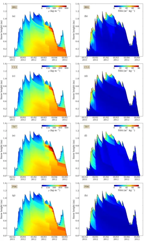
Figures 11–12 present, respectively, the simulated verti-cal profiles of density and SSA and the difference in terms of SSA between results obtained with different metamor-phism formulations. All the considerations we made for the 2009/2010 winter season still apply here. In particular, in
Fig. 11: Simulated density (left column) and SSA (right column) at Col de Porte during winter 2011/2012. Simulations were run using different metamorphism formulations. From top to bottom: B92 (Brun et al., 1992), C13 (this work), T07 (Taillandier et al., 2007) and F06 (Flanner and Zender,
2006). 39
Fig. 11. Simulated density (left column) and SSA (right column) at Col de Porte during the winter of 2011/2012. Simulations were run using different metamorphism formulations. From top to bottom: B92 (Brun et al., 1992), C13 (this work), T07 (Taillandier et al., 2007) and F06 (Flanner and Zender, 2006).
terms of density the discrepancies are negligible and in terms of SSA the results obtained using formulations C13 and B92 are similar. Moreover, SSA values computed with F06, even if generally consistent with those obtained with B92, tend to be lower in the upper layers. Lastly, the fact that during the melt period the snow height, SWE and albedo simulated using T07 remain higher than the other model results (see Fig. 10) can be explained by the large SSA values given by T07 during the dry and warm period between March and April 2012.
Fig. 12: Comparison in terms of SSA between the metamorphism formulations implemented into
Crocus. In order to compare results obtained using different formulations, all SSA profiles were
interpolated over a 1 cm vertical grid. The three plots show the difference between the new
formu-lations C13 (top), T07 (middle) and F06 (bottom) and the original formulation B92, for simuformu-lations
run at Col de Porte during winter 2011/2012. 40
Fig. 12. Comparison in terms of SSA between the metamorphism formulations implemented in Crocus. In order to compare results obtained using different formulations, all SSA profiles were inter-polated over a 1 cm vertical grid. The three plots show the differ-ence between the new formulations C13 (top), T07 (middle) and F06 (bottom) and the original formulation B92, for simulations run at Col de Porte during the winter of 2011/2012.
Fig. 13: Comparison between simulated and measured density (left) and SSA (right) at Col de Porte,
on 6 February 2012, 12h00 LT.
41
Fig. 13. Comparison between simulated and measured density (left) and SSA (right) at Col de Porte, on 6 February 2012, 12:00 LT.
down. All formulations estimate the snow height well and the simulated density values are in agreement with the ob-servations. The simulated SSA profiles are almost flat within the melt form layers and are able to capture the separation, at about 0.9 m above the ground, between older and more re-cent snow layers. However, some differences between model results appear at the surface: in the decomposed form layer SSA values from F06 are lower, whereas in the faceted crys-tal layer SSA values from T07 are higher.
4.3 Quantitative comparison between simulations and observations
The visual comparison between observed and simulated SSA profiles was complemented and consolidated by computing the quantity1SSA (see Sect. 3.5). 1SSA values for Col de Porte were computed with and without stretching vertically the simulated profiles, in order to match the measured snow height (in practice, according to Morin et al. (2013) the thick-ness of each numerical layer was linearly scaled with the ra-tio between observed and simulated total snow height). In the same way, correlation statistics were also performed in terms of optical diameter by computing the quantity1dopt.
Due to the inverse relationship between SSA and optical di-ameter (Eq. 1),1 values computed with one of these two related variables are sensitive to the model performance in a different way. Good predictions for high SSA values, for in-stance, have more impact on1SSAthan on1dopt; in contrast,
statistics expressed in terms of optical diameter will favour the model performances for the lower range of SSA values (Mary et al., 2013; Morin et al., 2013).
The results for1SSA and1dopt are presented in Fig. 14.
F06 give median values of1dopt between 0.09 and 0.12 mm
for Summit, between 0.36 and 0.42 mm for Col de Porte in 2009/2010 and between 0.55 and 0.71 mm for Col de Porte in 2011/2012. Summarising, we can state that, regardless of the formulation chosen, the high SSA are estimated better for the 2011/2012 season at Col de Porte than for the other data sets, whereas the low SSA are better simulated at Summit.
1SSA simulated using formulation T07 are consistent with those of the other formulations and1doptare even lower, with
median values of 0.35 and 0.34 mm for the 2009/2010 and 2011/2012 Col de Porte winter seasons, respectively. Lastly, it could be noticed that the vertical stretching of the simu-lated profiles does not improve significantly the agreement between the measured and observed values of SSA and the optical diameter.
5 Discussion
In the SURFEX/ISBA-Crocus multi-layer snowpack model, the snow metamorphism can now be described in terms of the rate of change of dopt, the optical diameter of snow. This makes Crocus different from any other existing detailed snowpack model. In SNOWPACK (Lehning et al., 2002), for instance, the snow microstructure is characterised by the grain geometric radius, whose growth is driven by the water vapour gradient between ice matrix and pore space, and by the dendricity and sphericity, which follow the same evolution laws used by Crocus; in addition, SNOWPACK also incorporates a representation of bonds between grains. The SMAP model (Niwano et al., 2012) employs the same variables and the same equations as those used in SNOW-PACK. The implementation of the optical diameter as a com-pletely prognostic variable constitutes a different approach compared to that followed in previous works, in which SSA was estimated from other prognostic variables (Jacobi et al., 2010; Morin et al., 2013; Roy et al., 2013b). This enables Crocus initialisations with an observed SSA profile and makes it possible to run the model using various parameteri-sations of SSA decay.
The original Crocus metamorphism formulation (B92), based on empirical evolution laws of grain dendricity, sphericity and size, already led to a satisfactory agreement between simulated and observed SSA values, considering that the accuracy of the SSA measurements is estimated to be about 10 % (Gallet et al., 2009; Arnaud et al., 2011). Using B92, we found median values of 1SSA lower than 10 m2kg−1 both at Summit and at Col de Porte. The new formulation using sphericity and optical diameter (C13), in which the rate of change ofdopt is deduced from the same equations as B92, also leads to maximum1SSAmedian val-ues of less than 10 m2kg−1. The fact that B92 and C13 give quite similar results in terms of SSA means that the opti-cal diameter has been integrated successfully into Crocus as a prognostic variable. In terms of 1SSA, the model
devel-Fig. 14. Comparison between simulations and observations in terms of1SSA(left column) and1dopt (right column). (a, b)1values
computed for Summit. (c, d)1values computed for Col de Porte during the winter of 2009/2010. (e, f)1values computed for Col de Porte during the winter of 2009/2010, in which simulations were stretched vertically in order to match the measured snow height. (g, h) Same as (c, d) for the winter of 2011/2012. (i, j) Same as (e, f) for the winter of 2011/2012.
is consistent with the recent study of Schleef and Loewe (2013), who found that the rate of decrease of the SSA un-der isothermal conditions, computed on micro-tomographic images, was independent of the density. At Col de Porte, the parameterisation proposed by Taillandier et al. (2007) (T07) gives median values of 1SSA that never exceed 8 m2kg−1 and are consistent with those of the other formulations. This means that, regardless of the formulation chosen, high SSA values are simulated well. During melt periods, SSA values from T07 remain relatively higher than those obtained using B92, C13 or F06. This leads to higher snow height, SWE and albedo values and also results in a better agreement between measured and simulated optical diameters.
Apart from some minor differences, formulations B92, C13, T07 and F06 lead to similar results in terms of simu-lated SSA. The statistical agreement between measured and simulated SSA profiles is rather satisfactory and compara-ble to previous studies. Morin et al. (2013), for instance, car-ried out simulations using Crocus and two parameterisations of snow SSA, one determined from density and snow type and the other one simply derived from the internal computa-tion of the optical radius in Crocus. In both cases, comparing simulations with SSA measurements in an Alpine environ-ment, they found RMSD values of 10 m2kg−1. Jacobi et al. (2010) implemented a parameterisation in Crocus in which the SSA was estimated from other snow variables using the equations of Taillandier et al. (2007). Comparing their re-sults against measurements in a dry subarctic snowpack at Fairbanks (Alaska), they observed generally good agreement between simulated and measured SSA, with RMSD ranging from 8 to 11 m2kg−1. These values are close to our findings. Density and optical diameter are not sufficient to charac-terise the snow microstructure uniquely. A notion of shape has to be introduced to account for different degrees of roundness from the entirely angular crystals, such as depth hoar, to the mostly rounded grains, such as melt forms. This need for a third variable to describe the snow microstruc-ture completely can also be made clearer by looking at the two-point correlation function of the microscopic density. In-deed, the first orders of the expansion of this function at the origin are linked not only to the volume fraction and the sur-face area per unit volume, but also to the curvature (Torquato, 2002; Löwe et al., 2011). Moreover, a good characterisation of the crystal shapes in snowpack models has proven to be important for several applications, such as the evaluation of the stability of the snow layers for avalanche forecasting (Du-rand et al., 1999) and the study of the transmission of light through snow (Meirold-Mautner and Lehning, 2004; Libois et al., 2013). For this reason, the notion of sphericity present in the original Crocus formulation still remains in the current version of the model. However, in the same way in which we replaced two semi-empirical quantities (dendricity and size) with the optical diameter, in the future it is desirable to re-place the sphericity with some other fully fledged physical variable easily measurable in the field. A possible candidate
to discriminate between different grain shapes seems to be the ratio of the vertical to the horizontal component of the thermal conductivity. This anisotropy of the thermal conduc-tivity ranges from 0.7 for rounded grains up to 1.5 for faceted crystals (Calonne et al., 2011). Unfortunately, for now this quantity can only be computed by micro-tomography and only a very limited data set is available. Recently, Libois et al. (2013) studied the impact of the grain shape on the macro-scopic optical properties of snow. In their approach, the snow particle shape is fully defined by two quantities, the absorp-tion enhancement parameter, quantifying the enhancement of absorption due to lengthening of the photon paths within the grain, and the geometric diffusion term, accounting for the angular anisotropy in diffused light. These quantities are both independent of the size and the former can be retrieved from reflectance and extinction measurements. They might con-stitute a possible alternative to the sphericity to describe the grain shape. When the sphericity will be replaced by one or more quantities which can be measured readily in the field and linked objectively to other relevant snow properties, then the snow microstructure in Crocus will be characterised in an entirely physical manner.
6 Conclusions
A new approach to describe snow metamorphism has been implemented in the SURFEX/ISBA-Crocus model. The op-tical diameter of snow, so far estimated indirectly from other state variables, has been turned into a prognostic variable and different parameterisations of its rate of change have been tested, by comparing results of simulations to field measure-ments. Characteristics and limits of such parameterisations have been discussed. Results indicate that all metamorphism formulations perform well in terms of simulated SSA, with median values of the RMSD between observed and simulated SSA lower than 10 m2kg−1.
description of the surface hoar formation, may be developed and evaluated with estimates of SSA from remote sensing.
Supplementary material related to this article is
available online at http://www.the-cryosphere.net/8/417/ 2014/tc-8-417-2014-supplement.pdf.
Acknowledgements. CNRM-GAME/CEN and LGGE are part
of Labex OSUG@2020 (ANR10 LABX56). This work was funded by INSU/LEFE project QUASPPER. The Summit field campaign was funded by grant no. 1088 from French Polar Institute (IPEV) to F. Domine and by grant no. 1023227 from National Science Foundation (NSF) to M. Bergin. We thank K. Steffen and N. Bayou for providing the AWS data for Summit, M. Flanner for providing his algorithm describing the evolution of effective radius and J.-M. Willemet for help in programming. We also wish to thank A. Royer, H. Loewe, E. Brun and M. Dumont for useful discussions and M. Lehning and an anonymous referee for helpful and constructive reviews
Edited by: E. Larour
The publication of this article is financed by CNRS-INSU.
References
Albert, M. and Hawley, R.: Seasonal differences in surface en-ergy exchange and accumulation at Summit, Greenland, Ann. Glaciol., 31, 387–390, 2000.
Albert, M. R. and Shultz, E. F.: Snow and firn properties and air-snow transport processes at Summit, Greenland, Atmos. Envi-ron., 36, 2789–2797, 2002.
Arnaud, L., Picard, G., Champollion, N., Domine, F., Gallet, J.-C., Lefebvre, E., Fily, M., and Barnola, J.-M.: Measurement of ver-tical profiles of snow specific surface area with a 1 cm resolution using infrared reflectance: instrument description and validation, J. Glaciol., 57, 17–29, doi:10.3189/002214311795306664, 2011. Barret, M., Domine, F., Houdier, S., Gallet, J.-C., Weibring, P., Walega, J., Fried, A., and Richter, D.: Formaldehyde in the Alaskan Arctic snowpack: partitioning and physical processes involved in air-snow exchanges, J. Geophys. Res., 116, D00R03, doi:10.1029/2011JD016038, 2011.
Brucker, L., Picard, G., Arnaud, L., Barnola, J.-M., Schneebeli, M., Brunjail, H., Lefebvre, E., and Fily, M.: Modeling time series of microwave brightness temperature at Dome C, Antarctica, using vertically resolved snow temperature and microstructure mea-surements, J. Glaciol., 57, 171–182, 2011.
Brun, E.: Investigation on wet-snow metamorphism in respect of liquid-water content, Ann. Glaciol., 13, 22–26, 1989.
Brun, E., Martin, E., Simon, V., Gendre, C., and Coléou, C.: An energy and mass model of snow cover suitable for operational avalanche forecasting, J. Glaciol., 35, 333–342, 1989.
Brun, E., David, P., Sudul, M., and Brunot, G.: A numerical model to simulate snow-cover stratigraphy for operational avalanche forecasting, J. Glaciol., 38, 13–22, 1992.
Brun, E., Martin, E., and Spiridonov, V.: Coupling a multi-layered snow model with a GCM, Ann. Glaciol., 25, 66–72, 1997. Calonne, N., Flin, F., Morin, S., Lesaffre, B., du Roscoat, S. R., and
Geindreau, C.: Numerical and experimental investigations of the effective thermal conductivity of snow, Geophys. Res. Lett., 38, L23501, doi:10.1029/2011GL049234, 2011.
Calonne, N., Flin, F., Geindreau, C., Lesaffre, B., and Rolland du Roscoat, S.: Study of a temperature gradient metamorphism of snow from 3-D images: time evolution of microstructures, phys-ical properties and their associated anisotropy, The Cryosphere Discuss., 8, 1407–1451, doi:10.5194/tcd-8-1407-2014, 2014. Carmagnola, C. M., Domine, F., Dumont, M., Wright, P., Strellis,
B., Bergin, M., Dibb, J., Picard, G., Libois, Q., Arnaud, L., and Morin, S.: Snow spectral albedo at Summit, Greenland: measure-ments and numerical simulations based on physical and chemi-cal properties of the snowpack, The Cryosphere, 7, 1139–1160, doi:10.5194/tc-7-1139-2013, 2013.
Colbeck, S. C.: Ice crystal morphology and growth rates at low su-persaturations and high temperatures, J. Appl. Phys., 54, 2677– 2682, 1983.
Conger, S. M. and McClung, D. M.: Comparison of density cutters for snow profile observations, J. Glaciol, 55, 163–169, 2009. Dee, D. P., Uppala, S. M., Simmons, A. J., Berrisford, P., Poli,
P., Kobayashi, S., Andrae, U., Balmaseda, M. A., Balsamo, G., Bauer, P., Bechtold, P., Beljaars, A. C. M., van de Berg, L., Bid-lot, J., Bormann, N., Delsol, C., Dragani, R., Fuentes, M., Geer, A. J., Haimberger, L., Healy, S. B., Hersbach, H., Hólm, E. V., Isaksen, L., Kålberg, P., Köhler, M., Matricardi, M., McNally, A. P., Monge-Sanz, B. M., Morcrette, J.-J., Park, B.-K., Peubey, C., de Rosnay, P., Tavolato, C., Thépaut, J.-N., and Vitart, F.: The ERA-Interim reanalysis: configuration and performance of the data assimilation system, Q. J. Roy. Meteor. Soc., 137, 553–597, doi:10.1002/qj.828, 2011.
Dominé, F. and Shepson, P. B.: Air-snow interactions and atmo-spheric chemistry, Science, 297, 1506–1510, 2002.
Domine, F., Taillandier, A.-S., and Simpson, W. R.: A parameteri-zation of the specific surface area of seasonal snow for field use and for models of snowpack evolution, J. Geophys. Res., 112, F02031, doi:10.1029/2006JF000512, 2007.
Domine, F., Albert, M., Huthwelker, T., Jacobi, H.-W., Kokhanovsky, A. A., Lehning, M., Picard, G., and Simp-son, W. R.: Snow physics as relevant to snow photochemistry, Atmos. Chem. Phys., 8, 171–208, doi:10.5194/acp-8-171-2008, 2008.
Domine, F., Gallet, J.-C., Bock, J., and Morin, S.: Structure, spe-cific surface area and thermal conductivity of the snowpack around Barrow, Alaska, J. Geophys. Res., 117, D00R14, doi:10.1029/2011JD016647, 2012.