www.the-cryosphere.net/8/1885/2014/ doi:10.5194/tc-8-1885-2014
© Author(s) 2014. CC Attribution 3.0 License.
Glacier area and length changes in Norway from repeat inventories
S. H. Winsvold1,2, L. M. Andreassen2, and C. Kienholz3
1Department of Geosciences, University of Oslo, P.O. Box 1047 Blindern, 0316 Oslo, Norway
2Section for Glaciers, Ice and Snow, Hydrology Department, Norwegian Water Resources and Energy Directorate, P.O. Box 5091 Majorstua, 0301 Oslo, Norway
3Geophysical Institute, University of Alaska Fairbanks, 903 Koyukuk Drive, Fairbanks, AK 99775-7320, USA
Correspondence to: S. H. Winsvold (s.h.winsvold@geo.uio.no)
Received: 7 May 2014 – Published in The Cryosphere Discuss.: 10 June 2014
Revised: 9 September 2014 – Accepted: 15 September 2014 – Published: 20 October 2014
Abstract. In this study, we assess glacier area and length changes in mainland Norway from repeat Land-sat TM/ETM+-derived inventories and digitized topographic maps. The multi-temporal glacier inventory consists of glacier outlines from three time ranges: 1947 to 1985 (GIn50), 1988 to 1997 (GI1990), and 1999 to 2006 (GI2000). For the northernmost regions, we include an additional inventory (GI1900) based on historic maps surveyed between 1895 and 1907. Area and length changes are assessed per glacier unit, 36 subregions, and for three main parts of Norway: south-ern, central, and northern. The results show a decrease in the glacierized area from 2994 km2in GIn50to 2668 km2in GI2000 (total 2722 glacier units), corresponding to an area reduction of−326 km2, or −11 % of the initial GIn50area. The average length change for the full epoch (within GIn50 and GI2000) is−240 m. Overall, the comparison reveals both area and length reductions as general patterns, even though some glaciers have advanced. The three northernmost sub-regions show the highest retreat rates, whereas the central part of Norway shows the lowest change rates. Glacier area and length changes indicate that glaciers in maritime areas in southern Norway have retreated more than glaciers in the interior, and glaciers in the north have retreated more than southern glaciers. These observed spatial trends in glacier change are related to a combination of several factors such as glacier geometry, elevation, and continentality, especially in southern Norway.
1 Introduction
Glaciers are key indicators of climate change, making their monitoring important (e.g., Vaughan et al., 2013). Remote sensing techniques are ideal for measuring glaciers on a large scale, as they cover remote glacierized areas with rela-tively little effort. Optical images provided by the Landsat TM/ETM+, Terra ASTER, or SPOT HRS have proven to be very efficient for mapping glacier extents (e.g., Paul et al., 2002, 2007; Paul and Kääb, 2005; Bolch et al., 2010; Nuth et al., 2013). Glacier outlines are typically obtained from satellite images using thresholded multispectral band ratios (Bayr et al., 1994; Sidjak and Wheate, 1999; Paul and Kääb, 2005; Kargel et al., 2014). An important advantage of the Landsat TM/ETM+ sensors is their large swath width, which is ideal for mapping extensive glacier regions.
Glacier inventory data are used for modeling glacier mass balance (e.g., Marzeion et al., 2012; Radi´c and Hock, 2013), estimating ice volumes (e.g., Huss and Farinotti, 2012; Grinsted, 2013; Andreassen et al., 2014), or predicting global sea level rise (e.g., Leclercq et al., 2011; Gregory et al., 2013).
lack information about the spatial and temporal variations of glacier change.
Previous glacier inventories of Norway from the 1960s to the 1980s lack digital glacier outlines (Østrem and Ziegler, 1969; Østrem et al., 1973, 1988), and glacier area and length assessments are complicated, for example, by unknown ice divides. The most recent satellite-derived glacier inventory of Norway is based on Landsat TM/ETM+ (Andreassen et al., 2012b). It uses a GIS-based approach and is com-piled following the Global Land Ice Measurements from Space (GLIMS) guidelines (Kargel et al., 2005; Racoviteanu et al., 2010). This data set is a highly detailed digital base-line product ideal for glacier area and length change assess-ments (Andreassen et al., 2008; Paul and Andreassen, 2009; Paul et al., 2011). Glacier length measurements are con-sidered one of the most important ways to quantify glacier change in the future (Hoelzle et al., 2003). Historical length change observations can give much information about how glaciers respond to climate (Leclercq et al., 2014). The newly compiled Norwegian glacier inventory is available through the GLIMS database and as a published book (Andreassen et al., 2012b). Globally, areas with multi-temporal glacier outline data sets are rare (Kargel et al., 2014). Because long-term glacier change assessments are crucial for understand-ing glacier response to climate (Hoelzle et al., 2003), there is a need to complete such a multi-temporal glacier inventory.
For the first time, we present multi-temporal data sets de-rived from Landsat TM/ETM+ satellite images and topo-graphic maps for all glacierized areas in Norway. We per-form a glacier area and length change assessment which is based on three data sets from the time ranges of 1947 to 1985 (GIn50), 1988 to 1997 (GI1990), and 1999 to 2006 (GI2000). We compare in situ length change observations with length changes from automatically derived centerlines. We extend the data sets prior to GIn50 using older topographic maps, which allows us to conduct an extended glacier area and length assessment on five ice caps in northern Norway. Con-cerning the multi-spectral band ratio technique, we demon-strate that mapped glacier areas are sensitive to small vari-ations in the chosen ratio thresholds.
2 Study region
Mainland Norway extends from 58 to 71◦N and 5 to 31◦E and covers an area of 385 199 km2(Fig. 1a). The identified 2534 glaciers in the most recent glacier inventory have a total area of 2692±81 km2(using±3 % as uncertainty), covering 0.7 % of the area of Norway (Andreassen et al., 2012b). In the most recent glacier inventory, glacier complexes are divided into individual glacier units. These glacier units share com-mon divides if they are part of a glacier complex; otherwise they correspond to single glaciers without a drainage divide. The number of glacier units in the most recent glacier inven-tory is 3143. We divided the study area into three
geograph-Figure 1. (a) The study area, with Norwegian glaciers shown in blue. (b) Norway is bordered by the Norwegian Sea in the west.
ical parts: northern, central, and southern Norway, which were further split into 36 subregions (map in Fig. 2e).
Coastal regions in Norway have a warm and moist mar-itime climate, while the interior is drier and colder. Climate gradients along a west–east transect are pronounced, espe-cially in southern Norway. This west–east pattern is caused by the westerly winds and the Gulf Stream, together with the shading effect in the eastern parts due to the coastal mountains (Hanssen-Bauer et al., 2009). These climatic fac-tors contribute to warmer conditions in Norway compared to similar latitudes elsewhere in the world. Norway has a lati-tudinal gradient in terms of mean temperature and precipi-tation, which both decrease from south to north. However, along the coast, there is no pronounced variation on climate because of the ice-free Norwegian Sea, although Norwegian glaciers span over∼1500 km from south to north (Fig. 1b). The mean equilibrium-line altitude (ELA) of the glaciers in-creases inland, and dein-creases towards the north due to cli-matic differences (Andreassen et al., 2005).
Figure 2. Spatial representation of the data sets. (a) A subset of five ice caps in northern Norway outlined in the period 1895–1907 (GI1900). The location of the subset is indicated by the black rectangle in (b). (b) GIn50consists of 168 N50-map sheets based on aerial photographs within 1947–1985. (c) GI1990consists of nine Landsat TM4 and TM5 satellite scenes within 1988–1997. Glacier area not covered by suitable scenes is shown in red. (d) GI2000includes 12 Landsat TM5 and ETM+7 satellite scenes from 1999 to 2006. (e) Illustration of the division of northern, central, and southern Norway and the 36 glacier regions.
Glacier inventories of Norway were published in 1973 for northern Norway (Østrem et al., 1973) and 1969 and 1988 for southern Norway (Østrem and Ziegler, 1969; Østrem et al., 1988). The first complete and satellite remote-sensing-based inventory of Norway was published in 2012 (Andreassen et al., 2012b). In this paper, Norway refers to mainland Nor-way only. Area and length changes for Svalbard were re-cently published by Nuth et al. (2013).
3 Data and methods 3.1 Data set background
Our glacier inventory data are compiled using multi-spectral Landsat satellite data for the time periods GI2000and GI1990, topographic maps based on aerial photographs for GIn50, and analogue maps to extend glacier outlines further back in time (GI1900, prior to the GIn50 data set) (Fig. 2). In our analy-sis, we compare the data sets resulting in three epochs: full epoch (GIn50–GI2000), epoch 1 (GIn50–GI1990), and epoch 2 (GI1990–GI2000).
In epoch 1 and epoch 2, some glaciers had less than 10 years between the two data sets compared, corresponding to 12 % of the numbers of glaciers in both GI1990 and GI2000 (Table 1). Ideally, glacier inventories should be retrieved
Table 1. The maximum, minimum, and mean time span in years within each epoch. Note the calculated glacier change is weighted by the time span between two data sets for each single glacier. The mean time span in this table is not weighted, but gives the mean of the time span for all glaciers included in each epoch.
Maximum Minimum Mean
time span time span time span
Full epoch 54 14 32
Epoch 1 41 3 17
Epoch 2 18 6 12
in intervals of a few decades when used in change assess-ments in order to account for the glacier response time (Hae-berli, 2004). However, if a glacier region encounters very fast down-wasting of the glaciers, shorter mapping intervals can be used, which is the case for many Norwegian glaciers.
3.2 GI2000and GI1990– Landsat satellite imagery
The Landsat TM/ETM+satellite images have multiple ad-vantages compared to imagery from ASTER and SPOT due to (1) the larger swath width of Landsat; (2) better availabil-ity of Landsat images, as other optical satellites were not operational during the time periods; and (3) Landsat hav-ing freely available georeferenced and orthorectified satel-lite scenes. The year of satelsatel-lite acquisitions and the spatial coverage for the GI1990 and GI2000 data sets are presented in Fig. 2c and d. GI1990 and GI2000 span over periods of 9 and 7 years, respectively, as it proved impossible to map outlines for all Norwegian glaciers within 1 or a few years using Landsat TM/ETM+. This is due to a lack of cloud-free Landsat TM/ETM+satellite scenes as a result of Nor-way’s pronounced maritime climate. Seasonal snow cover, due to the high precipitation rates throughout all seasons, also makes satellite image interpretation challenging (Andreassen et al., 2008). Due to extensive cloud coverage, and partly also seasonal snow, full coverage for the GI1990 was not possi-ble. No usable scenes were available for Jostedalsbreen, Lo-foten/Hamarøy, and part of inner Troms (see Sect. 3.8 and Fig. 2c).
Prior to the derivation of glacier outlines from the Land-sat scenes, we carried out an accurate orthorectification and quality check of the images using PCI Geomatica©. The Landsat L1T/L1G-products were delivered orthorectified and often used as is after a quality check (Table 2). However, selected satellite images had to be orthorectified prior to the derivation of outlines due to insufficient quality of the L1T/L1G-products, especially in mountainous areas. The root-mean-square error (RMSE) values for both the pur-chased satellite scenes and the orthorectified ones had an accuracy of less than ∼30 m. We calculated the band ra-tios for the Landsat images by including the red band (TM3) and the shortwave infrared band (TM5). We decided to use
TM3
TM5 instead of TM4
TM5 for the glacier delineation following Andreassen et al. (2008) results from glacier outlines in Jo-tunheimen. They show that TM3
TM5 performed better for ice located in shadow- and for debris-covered ice compared to
TM4
TM5. The band ratio method uses threshold values optimized for each satellite scene. We used TM3
TM5 ≥t1, wheret1varied between 1.6 and 2.8. To improve results in shadowed ar-eas, we included an additional threshold on the blue band, TM1≥t2, wheret2is either 35 or 60, with some exceptions (Table 2) (Paul and Kääb, 2005; Paul and Andreassen, 2009). We applied a median filter on the glacier outlines to elim-inate individual glacier pixels. Outlines were further manu-ally corrected in the case of debris cover, glacier–lake inter-faces, clouds, or cast shadow which hampered the automatic mapping. Only very few outlines had to be corrected for de-bris cover since the glaciers in Norway are mostly dede-bris- debris-free. Lakes and seasonal snow misclassified as glaciers were masked out from the glacier outline product. We used
topol-ogy editing in ArcGIS© for the manual corrections and the delineations of ice divides. Topology rules allowed for fea-tures that share the same geometry to be updated simultane-ously. The methods of filtering, human inspection, and edit-ing of the data sets are described in the glacier inventory by Andreassen et al. (2012b).
3.2.1 Band ratio accuracy and threshold sensitivity The accuracy of the band ratio method and the sensitivity of the used threshold values are essential for change as-sessment of glaciers. Orthophotos from the same acquisition year as the satellite images are ideal for determining accu-racy, but are rarely available. In Jotunheimen, a mountain-ous region in southern Norway, glacier outlines were com-pared with orthophotos taken 1 year apart, and an area differ-ence of−2.4 % was found (Andreassen et al., 2008). Fischer et al. (2014) show that Landsat-derived outlines (year 2003; medium spatial resolution: 30 m) compared to orthopho-tos (year 2003; high spatial resolution: 50 cm) for eastern Switzerland show similar results, meaning there is compa-rable accuracy between the medium-resolution and high-resolution source data for glaciers >1 km2. On the other hand, they found for glaciers<1 km2 that the uncertainty of the outlines increased with decreasing glacier size. For debris-free glaciers, the band ratio method is robust and ac-curate (Albert, 2002; Paul et al., 2003) with an accuracy be-tween±2 and 5 % (e.g., Paul et al., 2013). Here, we oper-ate with an accuracy of±3 %, implying that the inventory of Norwegian glaciers has a total accuracy of 2692±81 km2 (Andreassen et al., 2012b) (2668±80 km2 for the glaciers included in GI2000). The automatic band ratio method and manual digitizations give similar results, but the band ratio method often obtains a smaller glacier area as it tends to ex-clude some mixed pixels (Paul et al., 2013).
The mapped glacier area depends strongly on the chosen threshold value. The sensitivity of selected threshold val-ues used on the ratio TM3
TM5 ≥t1and the additional blue band TM1≥t2have been investigated for 57 glacier units in west-ern Finnmark, northwest-ern Norway. A Landsat 5 TM satellite scene with good snow and cloud conditions from the year 2006 was used (Area code 12000 in Table 2). By calculat-ing the difference in number of pixels mapped for selected thresholds, a percentage difference of area relative to the ap-plied threshold is calculated (Fig. 3). We used TM3
TM5 ≥2.4 and TM1≥35 or 60 as reference threshold values (yield-ing a total of 69.3 and 65.6 km2respectively). The TM3
TM5 ra-tio thresholds range from 2.0 to 2.8, with increments of 0.2. There were some outliers strongly affecting the mean values of area change between the thresholds compared, and thus it is more representative to use median values (Fig. 3a).
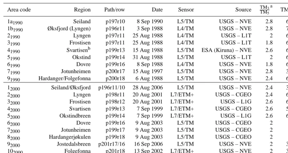
Table 2. Landsat satellite images for the GI1990and GI2000inventories. Dovre, Jotunheimen, and Hardangerjøkulen subregions were the first sites processed in GI2000, and did not include the TM1band (e.g., Andreassen et al., 2008) (L1G: image is from the Global Land Cover Facility (GLCF); L1T: standard terrain correction; NVE: Norwegian Water Resources and Energy Directorate; CGEO: Center for GIS and Earth Observation; ESA (Kiruna): European Space Agency (Kiruna ground station); USGS: US Geological Survey).
Area code Region Path/row Date Sensor Source TM3
TM5 a
TMa1
1a1990 Seiland p197r10 8 Sep 1990 L5/TM USGS – NVE 2.8 60
1b1990 Øksfjord (Lyngen) p196r11 3 Sep 1988 L4/TM USGS – NVE 2.8 70
21990 Lyngen p197r11 25 Aug 1988 L4/TM USGS – L1T 2 60
31990 Frostisen p197r11 25 Aug 1988 L4/TM USGS – L1T 1.8 60
41990 Svartisenb p199r13 15 Aug 1988 L5/TM ESA (Kiruna) – NVE 2.6 60
51990 Okstind p199r14 31 Aug 1988 L5/TM USGS – L1T 2 60
61990 Dovre p199r16 8 Sep 1988 L4/TM USGS – NVE 1.8 60
71990 Jotunheimen p200r17 15 Aug 1997 L5/TM USGS – NVE 2.8 35
91990 Hardanger/Folgefonna p200r18 6 Aug 1988 L5/TM USGS – NVE 2.4 60
12000 Seiland/Øksfjord p196r11/10 28 Aug 2006 L5/TM USGS – NVE 2.4 35
22000 Lyngen p198r11 20 Aug 2001 L7/ETM+ USGS – CGEO 2.4 60
32000 Frostisen p198r12 20 Aug 2001 L7/ETM+ USGS – L1G 2.6 60
42000 Svartisen p199r13 7 Sep 1999 L7/ETM+ USGS – CGEO 2.6 59
52000 Okstindbreen p199r14 7 Sep 1999 L7/ETM+ USGS – L1G 2.6 60
62000 Dovre p199r16 9 Aug 2003 L5/TM USGS – CGEO 2 –
72000 Jotunheimen p199r17 9 Aug 2003 L5/TM USGS – CGEO 2 –
82000 Hardangerjøkulen p199r18 9 Aug 2003 L5/TM USGS – CGEO 2 –
92000 Jostedalsbreen p201r17/16 16 Sep 2006 L5/TM USGS – NVE 2 35
102000 Folgefonna p201r18 13 Sep 2002 L7/ETM+ USGS – NVE 2 35
aValues are larger than or equal to the given treshold.bThe Blåmannsisen subregion used the threshold valuesTM3
TM5≥1.6and TM1≥35due to cirrus clouds.
glaciers in cast shadow). With lower threshold values, more noise was included, i.e., mixed pixels containing snow/ice and rock/debris. Similarly, when comparing TM3
TM5 ≥2.4 and 2.8 and TM1≥35, we find a median decrease in area of
−11 % (−3.1 km2). The higher threshold values used for TM3
TM5 reduce noise but include less glacier area compared to lower threshold values, due to fewer mixed pixels including both ice and terrain features. The TM3
TM5 threshold should be as low as possible so as to include the dirty ice around glacier perimeters (Paul et al., 2013). If TM3
TM5 ≥2.4 was used with TM1≥60, we found less variation when varying the thresh-old values compared to using the TM1≥35. This means a median area decrease of−4 % (−1.2 km2) usingTM3
TM5 ≥2.4 to 2.8 and a median area increase of 3 % using TM3
TM5 ≥2.0 to 2.4.
By applying a threshold of TM1≥35, the area mapped was more sensitive and included more mixed pixels com-pared to TM1≥60 (Fig. 3b and c). Glaciers in cast shadow were most sensitive to variations in the applied threshold, and manual on-screen digitization was necessary on some occa-sions.
3.3 GIn50– topographic maps
The GIn50 data set was derived by digitizing glacier out-lines from 168 first-edition 1:50 000 topographical maps
in the N50 series from the Norwegian Mapping Authority based on aerial photographs acquired between 1947 and 1985 (Fig. 2b). Digital form is required to conduct change analy-sis and to compare glacier drainage basins using the same drainage divides (Andreassen et al., 2008).
The first-edition N50-paper maps were scanned and geo-referenced using ground control points in a reference map (from European datum zone 32, 33, and 34 to WGS 84 UTM zone 33). The glacier outlines were then digitized on-screen. We used a first-order polynomial transformation and ob-tained RMSE values of less than 10 m. The years of the aerial photographs were provided by the Norwegian Mapping Au-thority, and the acquisition years were also checked on every map sheet. Some map sheets (e.g., 1532-2 Altevatnet) have several acquisition years, and thus the exact one is unknown (e.g., between 1947 and 1951). In those cases, the first map-ping year (e.g., 1947) was allocated to the glaciers within the map sheet.
Figure 3. (a) Box plot showing the relative area difference (%) for selected threshold values. The numbers in parentheses are outliers. (b) Visual representation of the threshold sensitivity for a part of Nordmannsjøkelen. The threshold sensitivity is represented in increments of 0.2 using TM3
TM5 ≥2.4 and TM1≥35 as the initial threshold value (black line). The blue frame indicates a glacier located in cast shadow. (c) TM3
TM5 ≥2.4 and TM1≥60 are used for the initial threshold value. Some of the smallest glaciers or possible snow fields are not even mapped when the threshold values are increased.
indicates little variation in the digitizing accuracy between the interpreters and minor effects on the end result. We ex-pect a larger uncertainty for the derivation of the actual out-lines on the maps. However, an uncertainty analysis was not applied to the topographic maps, because the orthorectifica-tion and digitizaorthorectifica-tion of the imagery would be a huge amount of work. Another uncertainty factor was the unknown work-ing methods and mappwork-ing principles of the cartographers of the time.
3.4 GI1900– analogue maps
The applicability of older analogue maps was tested in the two northernmost glacier regions in Norway (Seiland and Øksfjord; see Fig. 2a). A map series named Gradteigskart was used, which consists of quadrangle maps constructed from land surveys (map scale 1:100 000). The surveys of Seiland and Øksfjord were conducted in the period
analysis, the results must be interpreted with care and con-sidered as an estimate rather than an accurate benchmark.
For three composite glaciers in western Finnmark (Langfjordjøkelen, Øksfjordjøkelen, and Svartfjelljøkelen), we tested four transformation methods for georeferencing: (1) spline, (2) adjust, (3) second-order polynomial, and (4) third-order polynomial. We used 25 ground control points in each map sheet with a mean total RMSE of ±50 m. We chose to use the second-order polynomial as the transforma-tion method, as it had the best agreement with real topogra-phy and the other data sets. In total, the area of the second-order polynomial transformation method was 89 km2. Area differences between the tested methods varied up to 1.8 % (1.6 km2) relative to the applied method.
3.5 Digital elevation model (DEM)
A DEM is required for deriving topographic parameters, ice divides, and centerlines. We used GIS analysis to ex-tract glacier parameters from the data sets. Topographic par-ameters were calculated for GI2000, including minimum, maximum, mean, and median elevation; aspect; and slope. The spatial resolution of the DEM provided by the Norwe-gian Mapping Authority was 20 m, and the elevation con-tours, which the DEM was constructed from, were derived from aerial photography. The DEM from the Norwegian Mapping Authority was used for all ice divides, except on the Folgefonna and Hardangerjøkulen ice caps, where DEMs based on LIDAR data acquired in 2007 and 2010 were avail-able (Andreassen et al., 2012b). The national DEM was used to calculate the topographic parameters for all glaciers. Ac-cordingly, the date of the DEM is not always coincident with the date of the outlines. In the case of GI2000, the DEM data are up to∼20 years older than the outlines. Still, unless the elevation changes are very large, the surface changes have only a minor impact on many of the derived parameters due to the extensive number of pixels averaged when calculating slope, mean altitude, and aspect (Frey and Paul, 2012). How-ever, minimum elevation is sensitive to the applied DEM, as the minimum elevation is highly affected by rapid changes in the glacier termini. Ideally, we would have had multi-temporal DEMs, with each set of outlines having its own DEM, but this is not available for our study area. Paul et al. (2011) explored the possibility of using the ASTER global DEM in the Jostedalsbreen glacier region. The study revealed too many artifacts close to the termini of the glaciers, and concluded that the national DEM was a better choice.
3.6 Division of glaciers
To create an inventory of individual units, glaciers were di-vided into glacier units based on ice divides. We used the hydrology tools Flow Accumulation and Flow Direction in ArcGIS©. Flow Accumulation creates a raster of accumu-lated flow into each cell, and Flow direction finds the steepest
down slope neighbor for each cell. Both data sets are created from the national DEM. Additionally, discharge basins from the NVE were used to define ice divides manually. In the GI1900, GIn50, and GI1990, each glacier complex was sepa-rated using the same ice divide as GI2000. The glacier basins were adjusted to include glacier outlines from all three data sets. If GI1900, GIn50, and GI1990extended the GI2000 perime-ter, e.g., due to disintegrating glaciers, the ice divides and glacier basins were adjusted using topology editing and the DEM. In GI2000the 36 glacier regions were arranged from north to south (map in Fig. 2e), and, within the regions, glacier IDs (1–3143) were assigned automatically from north to south based on latitude. The Norwegian glacier inventory book includes maps and tables for all mapped glacier entities covered in GI2000(Andreassen et al., 2012b).
3.7 Deriving centerlines
Glacier length was reported for all glacier units in the pre-vious Norwegian glacier inventories (Østrem and Ziegler, 1969; Østrem et al., 1973, 1988). However, in the latest ventory of Norwegian glaciers, glacier length was not in-cluded (Andreassen et al., 2012b). In this study, we extend the inventory by adding glacier length.
We calculated centerlines by applying a three-step cost-grid–least-cost route approach which requires glacier out-lines and a DEM as input (Kienholz et al., 2014). We ex-cluded glaciers smaller than <1 km2 (from GIn50) to re-duce the noise from seasonal snow cover, which gives rel-atively large errors over smaller areas. Our method for deriv-ing centerlines was reproducible and fast compared to dig-itizing flow lines by hand, which would be very time con-suming. In the first step, the algorithm identifies the lowest glacier points as termini, while using local elevation maxima along the glacier outlines to identify heads for each major glacier branch. In the second step, the algorithm determines the actual centerlines between heads and termini by calculat-ing the least-cost route on a cost grid (Fig. 4). The cost grid is established using the grid cells’ elevations and Euclidean distances to the glacier edge. To allow for plausible center-lines, the lowest cost values are allocated to the glacier center and to lower glacier reaches. In the third step, the algorithm divides the centerlines into individual branches, which are then classified according to a branch order (Kienholz et al., 2014). Each step of the algorithm is implemented indepen-dently so that results can be checked visually and corrected if necessary.
Figure 4. GIn50and GI2000presented with the automatically derived glacier heads, termini, and centerlines at Øksfjordjøkelen.
in the case of glacier advance, or perpendicular shift of the termini relative to the original centerline. In these cases, the centerlines were manually lengthened following contour lines. Manual corrections were particularly important for the data set GI1900 due to often longer glacier lengths than in GIn50. The length change was derived from the length differ-ences of the centerlines. Tests indicated that this procedure yielded more plausible length changes than recalculating the centerlines for each period using the corresponding outlines. The main problem with such recalculation was that glacier recession often leads to the emergence of nunataks. The cen-terlines run around these new nunataks, increasing the glacier lengths, which interferes with the goal of isolating the change of the termini positions only.
In many cases the comparison between the centerlines from the glacier inventories was not feasible, preventing measurements of the length change. For example GI1900did not always align with the other data sets and in the case of Nordmannsjøkelen, only one out of nine glacier units could be used (Table 3).
Cumulative time series of glacier front position measure-ments were available from the NVE database, and we com-pared these in situ length change measurements with our length changes derived from centerlines for the full epoch. We used data from 12 glaciers with corresponding measur-ing periods in both the in situ measurements by the NVE and the cumulative length changes from topographic maps and satellite images derived in this study (Table 4). Additionally, five glaciers were compared for epoch 1, and six glaciers for
epoch 2. Some of the in situ measurements began before or after the GIn50first mapping year, but series were included if the gap was no larger than 5 years. Using an uncertainty of
±1 pixel for satellite images, variations less than 30 m can not be identified (Paul et al., 2011).
3.8 Inclusion, exclusion, and representation of data
Table 3. Glacier change within the whole period (GI1900and GI2000) for western Finnmark. Mean change, decadal mean change, and percentage total change.
Sample Mean Mean decadal Total change
change change (%)
Glacier A(n) L(n) A(km2) L(m) A(km2) L(m) Area Length
Nordmannsjøkelen (N) 9 1 −2.27 −1470 −0.32 −210 −91 −51
Seilandsjøkelen (Se) 6 4 −4.16 −1597 −0.59 −228 −71 −50
Langfjordjøkelen (L) 12 6 −0.95 −1231 −0.14 −187 −62 −43
Svartfjelljøkelen (Sv) 13 3 −0.34 −893 −0.05 −135 −46 −40
Øksfjordjøkelen (Ø) 17 12 −0.62 −795 −0.09 −120 −21 −27
All glaciers 57 26 −1.3 −1063 −0.19 −158 −53 −37
Table 4. Glacier length changes vs. in situ length changes. Engabreen is the only glacier with comparable data from northern Norway. The IDs refer to the glacier IDs in Andreassen et al. (2012b). For Midtdalsbreen (ID 2964), the measurements started in 1982, i.e., only epoch 2 was compared with in situ measurements for this glacier. Rembedalskåka (ID 2968) has discontinuous registrations in epoch 1 and 2. Five outlet glaciers from Jostedalsbreen (IDs: 2289, 2297, 2316, 2327, 2480) were not mapped in the GI1990data set, and for these glaciers, length changes are only calculated for the full epoch. Abbreviations: FE, full epoch; E1, epoch 1; E2, epoch 2; Na, not available.
In situ (m) Maps/satellite (m) Deviation (m)
Name (glacier ID) FE E1 E2 FE E1 E2 FE E1 E2 Pix.a Startb Periodc
Engabreen (1094) 149 19 130 256 147 109 107 128 21 4 1968 1968–1999
Fåbergstålsbreen (2289) −950 Na Na −624 Na Na 326 Na Na 11 1966 1966–2006
Nigardsbreen (2297) −268 Na Na −235 Na Na 33 Na Na 1 1967 1966–2006
Briksdalsbreen (2316) 25 Na Na 44 Na Na 19 Na Na 1 1966 1966–2006
Austerdalsbreen (2327) −197 Na Na −229 Na Na −32 Na Na −1 1966 1966–2006
Stigaholtbreen (2480) −705 Na Na −369 Na Na 336 Na Na 11 1966 1966–2006
Storbreen (2636) −60 −22 −38 −80 −18 −62 −20 4 24 −1 1980 1981–2003
Leirbreen (2638) −146 −92 −54 −143 −65 −78 3 27 24 0 1980 1981–2003
Styggedalsbreen (2680) −78 −64 −14 −66 −54 −12 12 10 −2 0 1981 1981–2003
Hellstugubreen (2786) −269 −222 −47 −228 −171 −57 41 51 10 1 1976 1981–2003
Midtdalsbreen (2964) Na Na −3 Na Na −50 Na Na 47 Na 1988 1988–2003
Rembedalskåka (2968) −55 Na Na −8 Na Na 47 Na Na 2 1971 1973–2003
aNumber of pixels that differs between the ground measured and remotely sensed measurements for the full epoch. The spatial resolution of the sensor pixel is 30 m. bStart year of the in situ data series included in this analysis. As close as possible to the start of the full epoch (topographic maps).
cThe years compared for the full epoch.
lower number of glaciers in the analyses for epoch 1 and 2 compared with the full epoch is insufficient satellite imagery due to cloud cover and seasonal snow for the GI1990 data set (see Sect. 3.2). Figure 2c presents the areas where data were lacking for GI1990. For example, during the Landsat TM 4/5 and ETM+ 7 operation period (1982–2012), the largest ice cap (Jostedalsbreen) in western Norway, where most of the data are missing, had only one Landsat satellite acquisi-tion with preferable mapping condiacquisi-tions (from 16 Septem-ber 2006). The mean area change for glaciers not overlap-ping in all epochs was−0.119 km2(2722 glacier units). In-cluding only glaciers overlapping in all epochs, mean area change was−0.096 km2(1684 glacier units). This variation indicates that Jostedalsbreen and glaciers in western Norway have been retreating.
Table 5. Glacier area change (GAC) for three parts of Norway and the change in the overall glacierized area for the three epochs. GAC(km2) represents the average change for all glacier units included in the analysis. Note: the glacier change is calculated for each individual glacier and its respective unique year difference before calculating the mean change.
Full epoch Epoch 1 Epoch 2
km2 % GAC(km2) km2 % GAC(km2) km2 % GAC(km2)
North −76.4 −16.5 −0.116 −87.4 −19.5 −0.141 17.7 4.7 0.023
Central −31.8 −4.0 −0.048 −83.2 −10.8 −0.145 56.9 8.3 0.092
South −218.0 −12.6 −0.156 −18.8 −3.2 −0.038 −41.8 −7.1 −0.073
Norway −326.1 −10.9 −0.12 −189.4 −10.5 −0.112 32.9 2.0 0.017
Table 6. Glacier length change (GLC) for three parts of Norway and the change in the overall glacierized area for the three epochs. GLC(m)represents the average change for all glacier units included in the analysis. Note: the glacier change is calculated for each indi-vidual glacier and its respective unique year difference before cal-culating the mean change.
Full epoch Epoch 1 Epoch 2
GLC(m) GLC(m) GLC(m)
North −357 −254 −82
Central −204 −221 −22
South −221 −129 −68
Norway −241 −199 −55
4 Results and discussion 4.1 Glacier area changes
The glacierized area in mainland Norway has decreased from 2994 km2 in GIn50 to 2668 km2 in GI2000, an area reduc-tion of−326 km2(−11 %) (Table 5). Although most glaciers were subject to area loss, 20 % of glaciers increased in area during the full epoch (in total 37 km2). For epoch 1, 19 % of glaciers increased in area, corresponding to 7.4 km2. In epoch 2, 63 % of glaciers gained area, corresponding to 98 km2. All in all, we find a clear decrease in glacier area for the full epoch (−10.9 %), as well as for epoch 1 (−10.5 %), but an increase in glacier area for epoch 2 (2 %) (Table 5). However, epoch 2 shows an area gain for the northern (4.7 %) and central parts (8.3 %), whereas the southern region de-creased in area (−7.1 %).
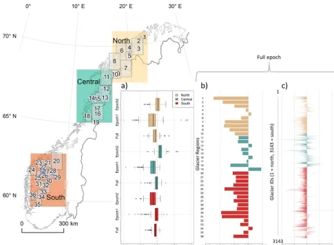
In Fig. 5, we present glacier area change for northern, cen-tral, and southern Norway for the full epoch using normal-ized values (rootGAC(A), whereAis the initial glacier area; Raup et al., 2009). This allows us to compare different groups with-out exaggerating the influence of the small glaciers, as is the case with values given in percentage, or the large glaciers, in the case of area changes given in absolute values (km2) (Raup et al., 2009) (see Sect. 4.5). In Fig. 5b and c, we find less glacier area decrease in the central part of Norway
(glacier regions 13–19) for the full epoch. In the northern-most glacier regions 1–4, we find the strongest retreat pat-tern of the Norwegian glaciers (Fig. 5b). This is in line with in situ observations from the only NVE-monitored ice cap in this area, Langfjordjøkelen (Glacier region 2), which shows a strongly negative mass balance and area reduction over the last few decades (Andreassen et al., 2012a). The trend of re-treating glaciers has also been seen on Svalbard, north of mainland Norway. Svalbard’s glaciers show a total area re-duction of−7 % in the last∼30 years (Nuth et al., 2013).
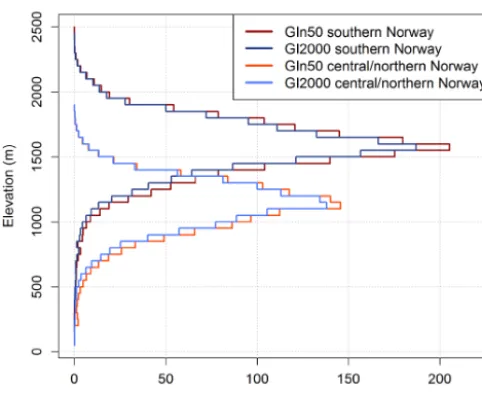
Glaciers in northern Norway are located at lower eleva-tions than glaciers in southern Norway. The distribution of area with elevation is presented in Fig. 6 for northern and southern Norway for the GIn50 and GI2000 data sets, illus-trating glacier area changes with elevation for the full epoch. Northern and central Norway are grouped because they show similar area–elevation distributions. For both southern and northern Norway, area decrease was larger at lower eleva-tions than at high elevaeleva-tions, with area changes observed at all elevations (Fig. 6). In the elevation range between 1000 and 1700 m a.s.l., corresponding to 62 % of the total eleva-tion range, the total absolute area loss is 201 km2. Many of the largest ice caps in both southern and northern Norway are located in this elevation range, and there are only a few glaciers that reach above 1700 m a.s.l.in central and northern Norway.
4.2 Glacier length changes
Figure 5. Glacier area change (GAC) ranging from north to south (a) displayed for Norway, (b) 36 glacier regions, and (c) 1–3143 glacier units. GAC is presented in rootGAC(A)(see Sect. 4.5). (a) Box plot showing the annual rootGAC(A) for three parts in Norway, and for three epochs. Only glaciers>0.5 km2are included in (a). (b) Mean annualrootGAC(A)for 36 glacier regions for the full epoch, and (c)rootGAC(A)for each glacier unit for the full epoch. Glacier regions and glacier units are arranged in a north–south order as defined in Andreassen et al. (2012b).
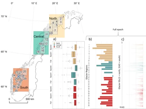
Glacier length changes show strong glacier retreat in all epochs and glacier regions, except for glacier region 19 in the full epoch (Fig. 7b). Overall, the length changes derived in this study show a steady retreat for many of the individ-ual glacier units even though some have advanced (Fig. 7c). It should be emphasized that different numbers of glaciers were compared in the glacier area change and glacier length change assessments because there are significantly less data on the glacier lengths than areas (see Sect. 3.8). This may explain the different patterns of change for epoch 2 (Figs. 5 and 7). Overall, length changes for the three parts of Norway show a retreat of the glaciers for all three epochs (Table 6).
4.2.1 Glacier length changes vs. in situ length changes
Comparison of our glacier length changes with cumulative field data from NVE for 12 selected glaciers shows a mean deviation of 89 m (<4 %) for the full epoch (Table 4), which
indicates that the satellite- and map-derived glacier length changes are in agreement for groups of glaciers, although the deviation can be relatively large for individual glaciers. Eight of the glaciers show good agreement (of±1 to 2 pixels) be-tween the length change methods.
Figure 6. Distribution of glacier area with elevation for GIn50and GI2000for all glaciers in Norway. We only compare glaciers present in both data sets. The clear bimodal distribution with a distinction between 1000 and 1350 m and 1400 and 1700 m illustrates the pdominant location of glaciers in northern and southern Norway, re-spectively (Andreassen et al., 2012b). Note that northern Norway includes the central and northern part presented in Figs. 5 and 7.
in front of the glacier and make it difficult to compare the measurements (Winkler et al., 2009). The determination of glacier terminus in cast shadow is limited by the quality and resolution of the satellite images used, causing uncertainties in the derived length change (Paul et al., 2011). In our case, Fåbergstølsbreen (glacier ID 2289) was actually located in cast shadow at the time of acquisition. The deviation can also be caused by differences in the measurement angle of the interpreter on the ground from a reference point toward the glacier and the path of the centerline used to derive length change from glacier outlines.
4.3 Glacier change since the beginning of the 1900s Using analogue maps from the beginning of the 1900s (GI1900), we extended the glacier area and length change as-sessments further back in time for five ice caps or former ice caps (Fig. 8). This glacier area change analysis included a total of 57 glacier units and 26 centerlines for glacier length analysis, all from these five ice caps (Table 3). One of the challenges in deriving glacier change in this region was dis-integrating glaciers, in particular Nordmannsjøkelen (Fig. 8). The glacier geometry changed extensively, including emerg-ing rock outcrops and ice patches separated from their trib-utaries. Strong thinning and retreat has been revealed for Langfjordjøkelen, one of the five ice caps, over the period 1966–2008 (Andreassen et al., 2012a).
In total, the five ice caps have decreased in area from 139 to 65 km2from the 1900s to 2006 (Fig. 8). The mean area
Table 7. Mean decadal area and length change from the beginning of the 1900s to the 2000s for five ice caps, divided into four epochs. We refer to the change between GI1900and GIn50as epoch 0. The “whole period” refers to the glacier change between GI1900 and GI2000. Note: averages were calculated using the set of decadal change values in each epoch for each glacier separately.
Epoch 0 Epoch 1 Epoch2 Whole period
Decadal
−0.13 −0.04 −0.03 −0.19 area change (km2)
Decadal
−73 −35 −42 −158 length change (m)
change from GI1900to GI2000(whole period) for the five ice caps is 1.3 km2(53 % in total), and the glacier length mea-surements show a mean retreat of 1063 m (37 % in total) (Ta-ble 3). The mean decadal changes for both area and length show the highest retreat rates for epoch 0 between GI1900 and GIn50with−0.13 km2(length change of−73 m). Epoch 1 and 2 show less relative retreat rates of−0.04 km2(length change of−35 m) and−0.03 km2(length change of−42 m), respectively (Table 7). Thus, these glaciers have been disin-tegrating and down-wasting extensively since 1900.
4.4 Spatial and temporal variation of glacier changes 4.4.1 Climate anomalies during the 20th century Our results show that glaciers in Norway have been receding between GIn50and GI2000, consistent with in situ data of in-dividual glaciers (Andreassen et al., 2005; Kjøllmoen et al., 2011). The data also show that maritime glaciers have been oscillating between periods of advance and recession, with recession being the most frequent state (Andreassen et al., 2005). The strong reduction in area and length in epoch 0 (GI1900to GIn50, Table 7) includes the warm period starting in the 1930s (Hanssen-Bauer, 2005), causing strong glacier retreat (Østrem and Haakensen, 1993; Andreassen et al., 2005; Andreassen et al., 2008).
Figure 7. Glacier length change (GLC) ranging from north to south (a) displayed for Norway, (b) 36 glacier regions, and (c) 1–3143 glacier units. (a) Box plot showing the annual GLC (m) for three parts of Norway, and for three epochs, and (b) mean annual GLC (m) for 36 glacier regions for the full epoch. Note that glacier regions 16, 18, and 30 do not include any glacier length data. (c) GLC (m) for each glacier unit for the full epoch. Glacier regions and the glacier units are arranged in a north–south order as defined in Andreassen et al. (2012b).
was observed between the mass gain and the related length change during the 1990s (Winkler et al., 2009).
4.4.2 Elevation
We did not find a significant relationship between average slope over each glacier unit and glacier length or area change for our data sets, although the data show a trend for less glacier change with increasing slope, as previously shown by Leclercq et al. (2014). Our results show that ice caps in northern Norway are particularly vulnerable to glacier area and length changes. Maritime glaciers are in general sensi-tive in Norway and retreat, but the glaciers in northern Nor-way retreat more because of less precipitation, warmer tem-peratures, and, for many glaciers, a location at lower eleva-tions (Figs. 6 and 8). These considerable changes are partly attributable to the glacier geometries: ice caps in Norway are relatively flat, and a high fraction of their surface re-mains close to the modern equilibrium line, which makes
them highly sensitive to climatic change (e.g., Nesje et al., 2008), whereas the steep glaciers are less sensitive. If the equilibrium line rises on ice caps, large parts of the accumu-lation area are transferred to the abaccumu-lation area, and the mass balance becomes strongly negative.
4.4.3 Climatic transects
Figure 8. Glacier area and length change for five ice caps in western Finnmark. The numbers after the mean percentage area and length change are the number of included glacier units (area) or centerlines (length). N: Nordmannsjøkelen; Se: Seilandsjøkelen; L: Langfjordjøkelen; Sv: Svartfjelljøkelen; and Ø: Øksfjordjøkelen.
“shadow” of the mountains in the east have less variation in glacier area and length change (Fig. 9). The mean winter balance on Gråsubreen is about 0.8 m water equivalent (w.e.), only∼20 % of the winter balance on Ålfotbreen (3.7 m w.e.) (Andreassen et al., 2005). Representing glacier area changes along a climatic transect illustrates the regional variation of glacier response to climate (Paul et al., 2007). Maritime glaciers have a high mass balance gradient compared to con-tinental glaciers. Due to global warming, glacier retreat will continue, and glaciers in maritime climates are expected to be more sensitive and respond more quickly than glaciers lo-cated in continental areas (Hoelzle et al., 2003). The drier continental glaciers are dependent on summer temperatures, while maritime glaciers are more sensitive to spring/fall tem-peratures (Oerlemans and Reichert, 2000).
Our analysis shows that glacier area and length changes are most pronounced for the northernmost glaciers (Figs. 5 and 7 and Tables 5 and 6). This agrees with geodetic and direct mass balance observations over the last decades. For example, the ice cap Langfjordjøkelen shows a stronger thin-ning and retreat than any other observed glacier in mainland Norway. Often the glacier has no accumulation area left at
the end of the mass balance year, and the accumulation-area ratio (AAR) was 0 % for many years during the 2000s (An-dreassen et al., 2012a). The ice cap simply does not have enough area at high altitude for the present climate.
Much of the annual variation in Norwegian climate is in-fluenced by the North Atlantic Oscillation (NAO) (Hurrell, 1995). Glaciers in Norway span a transect of ∼1500 km from south to north. Previous studies have shown that the NAO influences the winter and annual surface mass balance, but its effect is reduced towards more continental glaciers, as well as glaciers located at high latitudes (Nesje et al., 2000).
Figure 9. (a) Map of the west–east transect of glaciers in southern Norway. Å: Ålfotbreen; N: Nigardsbreen; and G: Gråsubreen. (b) Mean glacier change every 20 km from the coast for the full epoch is presented in box plots for yearly glacier area change (units of lengthrootGAC(A)). (c) Glacier length change (m). All glaciers are included for GAC, and glaciers>1 km2are included for GLC.
glacier, and the change signal of the small glacier is ampli-fied (Fig. 10b). When glacier change is expressed in terms of square-kilometer change, the opposite occurs. A large glacier losing the same area in terms of square kilometers as a small glacier with the same energy input will be overestimated in terms of the change signal, and the signal of small glaciers can be lost (Fig. 10a). Our solution for this was to express glacier area change in a length-scale dimension called units of length. This can be done by normalizing by the square root of the initial area, rootGAC(A), where GAC is glacier area change and A is the initial glacier area (Raup et al., 2009). With this normalization, we removed the systematic trend that depends on initial glacier size (Fig. 10c). By comparing this change
signal with glacier length change measurements derived from glacier centerlines, one obtains a similar distribution of the two change signals (Fig. 10d).
is not ideal for many Norwegian glaciers because of the many ice caps and cirque glaciers with often less distinct glacier termini.
5 Conclusions
We present a glacier area and length change analysis includ-ing multi-temporal data sets coverinclud-ing a larger area and higher temporal resolution than earlier studies. The glacierized areas in Norway are mapped from three glacier inventories within the period from 1947 to 2006. Overall, glacier area in main-land Norway decreased by−326 km2from GIn50to GI2000, corresponding to−11 %. The average glacier length change between GIn50and GI2000is−240 m. Glacier area and length changes indicate that glaciers in western Norway have re-treated more than in eastern parts, and northern glaciers have retreated more than southern glaciers. A combination of sev-eral factors like glacier geometry and elevation, as well as climatic aspects such as continentality, are related to the ob-served spatial trends in the glacier change analysis.
The change assessment based on historical maps going back to the 1900s in western Finnmark revealed a reduction in glacier area from a total of 139 to 65 km2, corresponding to a mean area and length change from GI1900to GI2000of
−53 % and−37 %, respectively.
Glacier outlines derived from topographic and historical maps have considerable uncertainties due to challenges re-lated to the seasonal snow cover. Therefore, the results show the upper bound of glacier changes in Norway. The results differ regionally, but clearly exhibit a main trend of retreat-ing glaciers between GIn50 and GI2000, even though some individual glaciers have advanced.
The increased availability of automatically derived and reproducible centerlines makes it easier to retrieve glacier length changes when multi-temporal glacier inventory data are available. Glacier length change derived from center-lines might be a more correct way to express glacier change signals due to reduced dependency on glacier geometries. Sensors with higher spatial and temporal resolution (e.g., the Sentinel-2 satellite) open new possibilities for observing glaciers in the future.
Author contributions. The design and data for the three inventories were created by L. M. Andreassen and S. H. Winsvold. L. M. An-dreassen and S. H. Winsvold developed the concepts of the study. C. Kienholz processed the centerlines for the multi-temporal data set. S. H. Winsvold prepared the final data and wrote the original manuscript with contribution from L. M. Andreassen.
SVALI. This publication is contribution number 43 of the Nordic Centre of Excellence SVALI, “Stability and Variations of Arctic Land Ice”, funded by the Nordic Top-level Research Initiative (TRI).
Acknowledgements. The study was supported by a PRODEX project of the European Space Agency (ESA) called CryoClim, supported by the Norwegian Space Agency. The study is also partly founded by the SVALI project. The authors would like to thank Holger Frey and the two anonymous reviewers for their thoughtful and detailed comments, which improved the paper significantly. We are very grateful to A. Kääb for guidance and suggestions to the work. Many thanks to C. Nuth (UIO) for input and feedbacks on the change analysis in general. Thanks to A. Voksø (NVE) for the design of the geodatabases and rules for topology editing of glacier outlines. Thanks to S. Engh for the manual digitization of the glacier outlines from the topographical maps in his summer job at NVE 2012. The main author appreciated the e-mail correspondence with Bruce Raup (NSIDC) regarding the discussion on alternative ways to represent glacier area change. And many thanks to Martin Hoelzle and Mauro Fischer from University of Fribourg for helpful comments. Thanks to Anna Sinisalo and John Burkhart from UIO for help with structure and language. Finally, thanks to all colleagues at UIO and NVE for helpful discussions.
Edited by: S. M. Noe
References
Albert, T. H.: Evaluation of remote sensing techniques for ice-area classification applied to the Tropical Quelccaya Ice Cap, Peru, Polar Geogr., 26, 210–226, 2002.
Andreassen, L. M., Elvehøy, H., Kjøllmoen, B., Engeset, R. V., and Haakensen, N.: Glacier mass-balance and length variation in Norway, Ann. Glaciol., 42, 317–325, 2005.
Andreassen, L. M., Paul, F., Kääb, A., and Hausberg, J. E.: Landsat-derived glacier inventory for Jotunheimen, Norway, and deduced glacier changes since the 1930s, The Cryosphere, 2, 131–145, doi:10.5194/tc-2-131-2008, 2008.
Andreassen, L. M., Kjøllmoen, B., Rasmussen, A., Melvold, K., and Nordli, Ø.: Langfjordjøkelen, a rapidly shrinking glacier in northern Norway, J. Glaciol., 58, 581–593, 2012a.
Andreassen, L. M., Winsvold, S. H., Paul, F., and Hausberg, J. E.: Inventory of Norwegian Glaciers, NVE report 38, 2012b. Andreassen, L. M., Huss, M., Melvold, K., Elvehøy, H., and
Winsvold, S. H.: Ice thickness measurements and volume esti-mates for glaciers in Norway, submitted, 2014.
Bayr, K. J., Hall, D. K., and Kovalick, W. M.: Observations on glaciers in the eastern Austrian Alps using satellite data, Int. J. Remote Sens., 15, 1733–1742, 1994.
Bolch, T., Menounos, B., and Wheate, R.: Landsat-based inventory of glaciers in western Canada, 1985–2005, Remote Sens. Envi-ron., 114, 127–137, 2010.
Cullen, N. J., Sirguey, P., Mölg, T., Kaser, G., Winkler, M., and Fitzsimons, S. J.: A century of ice retreat on Kilimanjaro: the mapping reloaded, The Cryosphere, 7, 419–431, doi:10.5194/tc-7-419-2013, 2013.
Frey, H. and Paul, F.: On the suitability of the SRTM DEM and ASTER GDEM for the compilation of topographic parameters in glacier inventories, Int. J. Appl. Earth Obs., 18, 480–490, 2012. GCOS: The Second Report on the Adequacy of the Global
Observ-ing Systems for Climate in Support of the UNFCCC, GCOS-82, World Meteorological Organisation, Geneva (WMO/TD No.1143), available at: http://www.wmo.int/pages/prog/gcos/ Publications/gcos-82_2AR.pdf (last access: 5 June 2014), 2003 GTN-G: The Global Terrestrial Network for Glaciers, available
at: http://www.gtn-g.org/about_gtng.html (last access: 6 August 2014), 2009
Gregory, J. M., White, N. J., Church, J. A., Bierkens, M. F. P., Box, J. E., van den Broeke, M. R., Cogley, J. G., Fettweis, X., Hanna, E., Huybrechts, P., Konikow, L. F., Leclercq, P. W., Marzeion, B., Oerlemans, J., Tamisiea, M. E., Wada, Y., Wake, L. M., and van de Wal, R. S. W.: Twentieth-century global-mean sea level rise: is the whole greater than the sum of the parts?, J. Climate, 26, 295–306, 2013.
Grinsted, A.: An estimate of global glacier volume, The Cryosphere, 7, 141–151, doi:10.5194/tc-7-141-2013, 2013. Haeberli, W.: Glaciers and ice caps: historical background and
strategies of worldwide monitoring, in: Mass Balance of the Cryosphere – Observations and Modelling of Contemporary and Future Changes, edited by: Bamber, J. L. and Payne, A. J., Cam-bridge University Press, CamCam-bridge, 559–578, 2004.
Hanssen-Bauer, I.: Regional temperature and precipitation series for Norway: analyses of time series updated to 2004, Met.no, Rep. 15/2005, 34 pp., 2005.
Hanssen-Bauer, I., Drange, H., Førland, E. J., Roald, L. A., Bør-sheim, K. Y., Hisdal, H., Lawrence, D., Nesje, A., Sandven, S., Sorteberg, A., Sundby, S., Vasskog, K., and Ådlandsvik, B.: Klima i Norge 2100, Bakgrunnsmateriale til NOU Klimatilplass-ing, Norsk klimasenter, September, 148 pp., 2009.
Hoel, A. and Werenskiold, W.: Glaciers and snowfields in Norway, Norsk Polarinstitutt Skrifter, Oslo, Norway, 114, 1962.
Hoelzle, M., Haeberli, W., Dischl, M., and Peschke, W.: Secular glacier mass balances derived from cumulative glacier length changes, Global Planet. Change, 36, 295–306, 2003.
Hurrell, J.: Decadal trends in the North Atlantic oscillation, Science, 269, 676–679, doi:10.1126/science.269.5224.676, 1995. Huss, M. and Farinotti, D.: Distributed ice thickness and volume
of all glaciers around the globe, J. Geophys. Res.-Earth, 117, F04010, doi:10.1029/2012JF002523, 2012.
Kargel, J. S., Abrams, M. J., Bishop, M. P., Bush, A., Hamilton, G., Jiskoot, H., Kääb, A., Kieffer, H. H., Lee, E. M., Paul, F., Rau, F., Raup, B., Shroder, J. F., Soltesz, D., Stainforth, D., Stearns, L., and Wessels, R.: Multispectral imaging contributions to global land ice measurements from space, Remote Sens. Environ., 99, 187–219, 2005.
Kargel, J. S., Leonard, G. J., Bishop, M. P., Kääb, A., and Raup, B.: Global Land Ice Measurements from Space, Series: Geophysical Sciences, Springer-Verlag, Berlin, Heidelberg, 810 pp., 2014. Kienholz, C., Rich, J. L., Arendt, A. A., and Hock, R.: A new
method for deriving glacier centerlines applied to glaciers in Alaska and northwest Canada, The Cryosphere, 8, 503–519, doi:10.5194/tc-8-503-2014, 2014.
Kjøllmoen, B. (Ed.), Andreassen, L., Elvehøy, H., Jackson, M, and Giesen, R. H.: Glaciological investigations in Norway in 2010, NVE report 3, 2011.
Leclercq, P. W., Oerlemans, J., and Cogley, J. G.: Estimating the glacier contribution to sea-level rise for the period 1800–2005, Surv. Geophys., 32, 519–535, 2011.
Leclercq, P. W., Oerlemans, J., Basagic, H. J., Bushueva, I., Cook, A. J., and Le Bris, R.: A data set of worldwide glacier length fluctuations, The Cryosphere, 8, 659–672, doi:10.5194/tc-8-659-2014, 2014.
Marzeion, B., Jarosch, A. H., and Hofer, M.: Past and future sea-level change from the surface mass balance of glaciers, The Cryosphere, 6, 1295–1322, doi:10.5194/tc-6-1295-2012, 2012. Moon, T. and Joughin, I.: Changes in ice front position on
Green-land’s outlet glaciers from 1992 to 2007, J. Geophys. Res.-Earth, 113, F02022, doi:10.1029/2007JF000927, 2008.
Nesje, A.: Briksdalsbreen in western Norway: AD 1900–2004 frontal fluctuations as a combined effect of variations in win-ter precipitation and summer temperature, Holocene, 15, 1245– 1252, 2005.
Nesje, A., Lie, Ø., and Dahl, S. O.: Is the North Atlantic Oscilla-tion reflected in Scandinavian glacier mass balance records?, J. Quaternary Sci., 15, 587–601, 2000.
Nesje, A., Bakke, J., Dahl, S. O., Lie, Ø., and Matthews, J. A.: Nor-wegian mountain glaciers in the past, present and future, Global Planet. Change, 60, 10–27, 2008.
Nuth, C., Kohler, J., König, M., von Deschwanden, A., Hagen, J. O., Kääb, A., Moholdt, G., and Pettersson, R.: Decadal changes from a multi-temporal glacier inventory of Svalbard, The Cryosphere, 7, 1603–1621, doi:10.5194/tc-7-1603-2013, 2013.
Oerlemans, J. and Reichert, B. K.: Relating glacier mass balance to meteorological data by using a seasonal sensitivity characteristic, J. Glaciol., 46, 1–6, 2000.
Østrem, G. and Haakensen, N.: Glaciers of Norway, in: Satellite image atlas of glaciers of the world, edited by: Williams, R. S. and Ferrigno, J. G., US Geological Survey, Professional Paper, 1386-E-3, 53 pp., 1993.
Østrem, G. and Ziegler, T.: Atlas over breer i Sør-Norge (Atlas of glaciers in South Norway), Hydrologisk avdeling, Norges Vassdrags- og Elektrisitetsvesen, Meddelelse, Oslo, Norway, 20, 207 pp., 1969.
Østrem, G., Haakensen, N., and Melander, O.: Atlas over breer i Nord-Skandinavia (Glacier atlas of Northern Scandinavia), Hydrologisk avdeling, Norges Vassdrags- og Energiverk, Med-delelse, Oslo, Norway, 22, 315 pp., 1973.
Østrem, G., Selvig, K. D., and Tandberg, K.: Atlas over breer i Sør-Norge (Atlas of glaciers in South Norway), Hydrologisk avdel-ing, Norges Vassdrags- og Energiverk, Meddelelse, Oslo, Nor-way, 61, 180 pp., 1988.
Paul, F. and Andreassen, L. M.: A new glacier inventory for the Svartisen region, Norway, from Landsat ETM+ data: challenges and change assessment, J. Glaciol., 55, 607–618, 2009. Paul, F. and Kääb, A.: Perspectives on the production of a glacier
in-ventory from multispectral satellite data in Arctic Canada: Cum-berland Peninsula, Baffin Island, Ann. Glaciol., 42, 59–66, 2005. Paul, F., Kääb, A., Maisch, M., Kellenberger, T., and Haeberli, W.: The new remote-sensing-derived Swiss glacier inventory: I. Methods, Ann. Glaciol., 34, 355–361, 2002.
Paul, F., Kääb, A., and Haeberli, W.: Recent glacier changes in the Alps observed by satellite: consequences for future monitoring strategies, Global Planet. Change, 56, 111–122, 2007.
Paul, F., Barry, R., Cogley, J. G., Frey, H., Haeberli, W., Ohmura, A., Ommanney, C. S. L., Raup, B., Rivera, A., and Zemp, M.: Rec-ommendations for the compilation of glacier inventory data from digital sources, Ann. Glaciol., 50, 119–126, 2009.
Paul, F., Andreassen, L. M., and Winsvold, S. H.: A new glacier inventory for the Jostedalsbreen region, Norway, from Landsat TM scenes of 2006 and changes since 1966, Ann. Glaciol., 52, 153–162, 2011.
Paul, F., Barrand, N. E., Baumann, S., Berthier, E., Bolch, T., Casey, K., Frey, H., Joshi, S. P., Konovalov, V., Bris, R. L., Molg, N., Nosenko, G., Nuth, C., Pope, A., Racoviteanu, A., Rastner, P., Raup, B., Scharrer, K., Steffen, S., and Winsvold, S.: On the accuracy of glacier outlines derived from remote-sensing data, Ann. Glaciol., 54, 171–182, 2013.
Racoviteanu, A. E., Paul, F., Raup, B., Khalsa, S. J. S., and Arm-strong, R.: Challenges and recommendations in mapping of glacier parameters from space: results of the 2008 Global Land Ice Measurements from Space (GLIMS) workshop, Boulder, Colorado, USA, Ann. Glaciol., 50, 53–69, 2010.
Radi´c, V., and Hock, R.: Glaciers in the Earth’s hydrological cycle: assessments of glacier mass and runoff changes on global and re-gional scales, Surv. Geophys., 35, 813–837, doi:10.1007/s10712-013-9262-y, 2013.
Rasmussen, L.: Spatial extent of influence on glacier mass balance of North Atlantic circulation indices, Terra Glacial., 11, 43–58, 2007.
Raup, B., Khalsa, S. J. S., Armstrong, R., and Racoviteanu, A.: The GLIMS Glacier Database: Status and Summary Analysis, MOCA09 – Our Warming Planet, IAMAS, IAPSO and IACS 2009 Joint Assembly, 2009.
Sidjak, R. W. and Wheate, R. D.: Glacier mapping of the Illecille-waet icefield, British Columbia, Canada, using Landsat TM and digital elevation data, Int. J. Remote Sens., 20, 273–284, 1999. Vaughan, D. G., Comiso, J. C., Allison, I., Carrasco, J., Kaser,
G., Kwok, R., Mote, P., Murray, T., Paul, F., Ren, J., Rig-not, E., Solomina, O., Steffen, K., and Zhang, T.: Observations: Cryosphere. In: Climate Change 2013: The Physical Science Ba-sis. Contribution of Working Group I to the Fifth Assessment Re-port of the Intergovernmental Panel on Climate Change, edited by: Stocker, T. F., Qin, D., Plattner, G. K., Tignor, M., Allen, S. K., Boschung, J., Nauels, A., Xia, Y., Bex, V., and Midgley, P. M., Cambridge University Press, Cambridge, United Kingdom and New York, NY, USA, http://www.climatechange2013.org/ images/report/WG1AR5_Chapter04_FINAL.pdf (last access: 31 July 2014), 2013.