https://doi.org/10.5194/amt-10-4639-2017 © Author(s) 2017. This work is distributed under the Creative Commons Attribution 3.0 License.
Using depolarization to quantify ice nucleating particle
concentrations: a new method
Jake Zenker1, Kristen N. Collier1, Guanglang Xu1, Ping Yang1, Ezra J. T. Levin2, Kaitlyn J. Suski2,a, Paul J. DeMott2, and Sarah D. Brooks1
1Department of Atmospheric Science, Texas A&M University, College Station, TX 77843, USA 2Department of Atmospheric Science, Colorado State University, Fort Collins, CO 80526, USA anow at: Pacific Northwest National Laboratory, Richland, WA 99352, USA
Correspondence to:Sarah D. Brooks ([email protected]) Received: 23 May 2017 – Discussion started: 12 July 2017
Revised: 5 October 2017 – Accepted: 8 October 2017 – Published: 1 December 2017
Abstract. We have developed a new method to determine ice nucleating particle (INP) concentrations observed by the Texas A&M University continuous flow diffusion chamber (CFDC) under a wide range of operating conditions. In this study, we evaluate differences in particle optical properties detected by the Cloud and Aerosol Spectrometer with PO-Larization (CASPOL) to differentiate between ice crystals, droplets, and aerosols. The depolarization signal from the CASPOL instrument is used to determine the occurrence of water droplet breakthrough (WDBT) conditions in the CFDC. The standard procedure for determining INP con-centration is to count all particles that have grown beyond a nominal size cutoff as ice crystals. During WDBT this procedure overestimates INP concentration, because large droplets are miscounted as ice crystals. Here we design a new analysis method based on depolarization ratio that can extend the range of operating conditions of the CFDC. The method agrees reasonably well with the traditional method under non-WDBT conditions with a mean percent error of ±32.1 %. Additionally, a comparison with the Colorado State University CFDC shows that the new analysis method can be used reliably during WDBT conditions.
1 Introduction
Ice clouds cover approximately 40 % of the Earth’s atmo-sphere (Wylie and Menzel, 1999). Because of their compli-cated microphysical properties, ice and mixed-phase clouds pose challenges in understanding our global radiative budget
and precipitation (Wendisch et al., 2005; Pinto, 1998; Yang et al., 2015; Korolev, 2007). Despite several decades of ef-fort by the atmospheric community to study ice clouds, there are still large gaps in our understanding of the impacts they have on our climate (Boucher et al., 2013). While experi-mental chambers have been used to study ice nucleation pro-cesses and ice nucleating particle (INP) concentrations for more than 30 years, INP measurement techniques are still under development.
Ice nucleation measurements are challenging for several reasons. The concentration of effective INPs is typically 0.1 to 1000 L−1or∼10−6to 10−4of the total aerosol concentra-tion (DeMott et al., 2003, 2015; Jiang et al., 2014; Mason et al., 2016; Cziczo et al., 2017). Secondly, differentiating be-tween ice crystals and droplets using particle discrimination methods is experimentally challenging. Thirdly, ice crystals can nucleate via several mechanisms (Vali, 1985; Vali et al., 2015), and accurate measurements must account for ice crys-tals initiated by each of these mechanisms.
al., 2011; Murray et al., 2012). In addition, when an aerosol forms a solution droplet below the melting point, condensa-tional freezing may occur. Finally, contact freezing occurs when an aerosol in contact with a water droplet surface initi-ates freezing. While the exact mechanism of contact freezing remains unresolved, it has been shown that the presence of an INP positioned at a droplet surface facilitates freezing at temperatures several degrees warmer than immersion freez-ing with identical INPs (Fornea et al., 2009; Brooks et al., 2014; Durant and Shaw, 2005). Knowledge of each of these mechanisms is important for understanding the formation of ice in mixed-phase clouds (containing droplets and ice crys-tals) and for developing robust parameterizations for global climate models (Tan et al., 2016; Pithan et al., 2014).
Composition, surface structure, and size are important fac-tors in determining the ice nucleating ability of an aerosol particle (Zolles et al., 2015; Niemand et al., 2012; Hoose and Möhler, 2012). Measurements suggest that K-feldspar, a common component of soil dust aerosol, may account for a large fraction of Earth’s INPs (Atkinson et al., 2013; Yakobi-Hancock et al., 2013). Recent investigations of other aerosols have identified aromatic pollutant aerosols, secondary or-ganic aerosols, marine aerosols, and aerosols produced from biomass burning as effective INPs (Brooks et al., 2014; De-Mott et al., 2016; McCluskey et al., 2014, 2016; Levin et al., 2016; Collier and Brooks, 2016).
Optical techniques have been used to detect and charac-terize ambient ice crystals (Mishchenko and Sassen, 1998; Yoshida et al., 2010; Noel and Sassen, 2005). For example, lidar observations use the depolarization ratio to distinguish cloud particle type (i.e., ice crystals or water droplets). In traditional lidar applications, the depolarization ratio is cal-culated using Eq. (1):
δLidar=B⊥ Bk
, (1)
where B⊥ andBk are the perpendicular and parallel
com-ponents of the lidar signal retrieved from the ambient at-mosphere or clouds. Under single scattering conditions, the depolarization ratio associated with an ensemble of water droplets is essentially zero while the counterpart for ice crys-tals is nonzero with a specific value depending on particle habit and orientation. Ice crystal depolarization ability is at-tributed to the high irregularities in the shapes and surfaces of ice crystals (Bohren and Huffman, 1983). The number of INPs present in a cloud can dictate its optical properties throughout the ice nucleation process (Hoose and Möhler, 2012; Murray et al., 2012).
Several previous studies have designed new analysis meth-ods for ice chambers that utilize the depolarization ratio mea-sured by optical particle counters (OPCs) (Glen and Brooks, 2014; Nicolet et al., 2010; Clauss et al., 2013; Garimella et al., 2016). Nicolet et al. (2010) accurately quantified ice crys-tals in the presence of water droplets in a chamber by using the peak intensity of the depolarization ratio to discriminate
between ice crystals and droplets with the Ice Optical DE-tector (IODE). Rather than using the peak intensity of the depolarization signal, Clauss et al. (2013) used the width of the pulse detected in the depolarization channel of the Thermo-stabilized Optical Particle Spectrometer for the de-tection of Ice (TOPS-ice) for phase discrimination. Alterna-tively, Garimella et al. (2016) used a machine learning tech-nique with scattering signals, including linear depolarization signals detected by an OPC installed in the SPectrometer for Ice Nuclei (SPIN, Droplet Measurement Technologies, Inc.) to determine INP concentration.
A continuous flow diffusion chamber (CFDC) designed to measure ice nucleation was originally developed by Rogers (1988) at the University of Wyoming and was later modified and rebuilt at Colorado State University (CSU). Several other ice nucleation chambers have been developed since then including the CFDC at Texas A&M University (TAMU) used in this study. Many enhancements have been made to ice nucleation chambers (e.g., Rogers et al., 2001; Creamean et al., 2013; DeMott et al., 2015; Prenni et al., 2013; Coluzza et al., 2017; Kanji et al., 2017), including replacement of the TAMU CFDC’s standard optical detec-tor (CLIMET, model no. CI-3100), which uses particle size to distinguish ice crystals from water droplets and aerosols, with the Cloud and Aerosol Spectrometer with POLariza-tion (CASPOL, Droplet Measurement Technologies, Inc.). The CASPOL detects forward scattering, backward scatter-ing, and depolarization on a single particle basis. In addi-tion, the CASPOL has been used to differentiate between ice crystals and various types of dust and soil particles based on backward scattering and depolarization signals (Glen and Brooks, 2013, 2014).
In this study, we demonstrate how differences in parti-cle optical properties can be used to differentiate between ice crystals, droplets, and aerosols detected by the CASPOL. In addition, we present a new method to quantify INP con-centrations detected by the TAMU CFDC using depolariza-tion ratio. Finally, INP concentradepolariza-tions obtained using the new method are compared with results obtained through the tra-ditional analysis method that primarily uses particle size to identify INP as well as INP concentrations reported by an-other ice nucleation chamber, the CSU CFDC.
2 Experimental
2.1 The TAMU CFDC and CASPOL
and Brooks, 2013, 2014; Glen, 2014). Hereafter, CFDC refers to the TAMU CFDC unless otherwise stated.
During operation, sample aerosols pass through a diffusion dryer to remove moisture from the air and before they enter the CFDC. Typically, aerosol flow is directed through a BGI Sharp Cut Cyclone impactor (model 0.732) prior to entering the CFDC in order to remove aerosols with a diameter greater than∼1.75 µm from the sample flow. However, the data pre-sented here were collected by the TAMU CFDC-CASPOL during the second phase of the Fifth International Ice Nu-cleation Workshop campaign (FIN-02) and no impactor was used during the campaign. Reasons for this choice were that the objective of FIN-02 was intercomparison with other in-struments that did not have impactors available, aerosol size distributions were well characterized, and supermicron parti-cle numbers were small.
Next, aerosols enter the CFDC processing chamber where temperature and supersaturation are controlled. The process-ing chamber consists of two concentric cylindrical walls coated with ice. Separate refrigeration units on each wall can be controlled to create a temperature gradient in the chamber that imposes a region of supersaturation with respect to ice (SSi)in the CFDC. The CFDC chamber is 75 cm long. The bottom 25 cm of the walls is coated with hydrophobic Teflon to prevent water from freezing to the wall in this region. This section of the chamber is referred to as the evaporation re-gion because it remains subsaturated with respect to water and partially or completely evaporates any water droplets that nucleate in the CFDC. The separate wall temperatures are manually controlled and monitored through a LabVIEW pro-gram. The temperature and supersaturation conditions at the position of the sheath air surrounded aerosol lamina are cal-culated using analytical equations reported in Rogers (1988). Before measurements can be taken with the CFDC, the processing chamber must be prepared. First, a vacuum pump is used to evacuate the chamber for approximately 30 min in order to eliminate ambient aerosols that may have infiltrated the chamber and to remove moisture that may cause the walls to accumulate an uneven coating of ice or allow ice to accu-mulate in other sensitive regions. The walls are then cooled to a temperature of−25◦C and the CFDC walls are iced by pumping Nanopure water into the chamber from the base. Excess water is drained out of the instrument for approxi-mately a minute after icing is complete. Then, the chamber is evacuated and refilled with N2gas once more before sam-pling is initiated.
At the base of the processing chamber, particles pass through a detector to determine INP concentration. In pre-vious TAMU CFDC studies, either an OPC (Climet, Inc.) or the CASPOL were employed (Glen and Brooks, 2014; McFarquhar et al., 2011). During FIN-02, the CASPOL was the chosen detector. Two mass flow controllers downstream of the CASPOL are used to set the total flow and recircu-lating sheath flow through the CFDC-CASPOL. The differ-ence between the total and sheath flows determines the
sam-ple flow. For this campaign, the total flow was set to values ranging from 6 to 9 L min−1and the sheath flow was set to values ranging from 4 to 7 L min−1, resulting in a sample flow that was typically∼2±0.5 L min−1. During operation, the CFDC made scans from low to high supersaturation at a constant aerosol lamina temperature (±1.5◦C). This is ac-complished by increasing wall temperature difference in a manner that retains the desired temperature at the position of the aerosol lamina.
The CASPOL (Droplet Measurement Technologies, Inc.) is a prototype particle-by-particle counter. Laser light (680 nm) is scattered by single particles entering the CASPOL and detected by three detectors that give informa-tion about the optical properties: a forward scatter detector, a backward scatter detector with a parallel polarized filter, and a backward scatter detector with a perpendicular polar-ized filter. Particles are spolar-ized according to the intensity of light, which reaches the CASPOL’s forward scatter detector, as in a traditional OPC. The forward scattering detector of the CASPOL registers particles on an individual basis and sorts those particles into a series of size bins ranging from 0.6 to 50 µm optical diameter. In addition, the instrument has a fourth detector that determines whether a particle is prop-erly aligned in the laser beam and should thus be recorded.
The depolarization ratio derived from CASPOL measure-ments is defined as follows (Glen and Brooks, 2014): δCAS=
B⊥,CAS B⊥,CAS+Bk,CAS
, (2)
where B⊥,CAS and Bk,CAS denote the signals from the CASPOL’s perpendicular and parallel backward scattering detector, respectively. This definition differs somewhat from the conventional depolarization ratio used in remote sensing based on lidar observations. The main difference is that the CASPOL detects light at the back scattering angles of 168 to 176◦rather than precisely 180◦in the case of lidar. Also, the
CASPOL occasionally detects a particle for which the paral-lel backscatter signal is below the limit of detection and thus is registered as zero, while the same particle has a nonzero perpendicular signal. In such cases, the calculated lidar de-polarization ratio of such particles is of spurious singularity. In contrast, the value of depolarization ratio calculated by Eq. (2) in the aforementioned case yields a value of unity, making the depolarization ratio of these particles quantita-tively meaningful. Likewise, in cases where the perpendicu-lar backscatter is below the limit of detection, the reported depolarization ratio is also unity.
2.2 Data collection during FIN-02
campaign: the Aerosols Interaction and Dynamics in the At-mosphere (AIDA) chamber and the Aerosol Preparation and Characterization (APC) chamber. The AIDA chamber can be used to simulate atmospheric conditions that give rise to cloud particle formation and growth and has been used in many previous campaigns and instrument intercompar-isons to examine the ice nucleating ability of various aerosols (Amato et al., 2015; Schnaiter et al., 2016; Wagner et al., 2015; DeMott et al., 2011). The AIDA chamber is a three-story, 84 m3 volume chamber that uses adiabatic expansion to simulate the atmospheric conditions required for ice nu-cleation to occur. During FIN-02, aerosols were drawn from the AIDA chamber by the various ice nucleation instruments prior to expansion. Following the aerosol sampling period, an AIDA expansion was performed so that INP concentra-tion determined by AIDA could be compared to results from the various visiting instruments. The second chamber, the APC, is a 3.7 m3volume chamber in which aerosols of a se-lected composition are produced by atomization and solid aerosol generation methods, suspended in dry synthetic air, uniformly distributed with a mixing fan, and maintained at constant temperature and pressure (Linke et al., 2006). While the APC lacks the adiabatic expansion capabilities of AIDA, the APC was used during FIN02 to provide a uniformly high concentration of aerosols of various compositions. Samples were subsequently distributed to the participating ice nucle-ation instruments.
During the campaign groups from 22 institutions sampled both the AIDA and APC chambers using a variety of online and offline ice nucleation measurement techniques. For ver-ification of the TAMU CFDC-CASPOL measurements and new analysis method, we compare our results to the mea-surements of the CSU CFDC. In order to test the CASPOL detector response to ice and non-ice particles, auxiliary mea-surements of olive oil droplets, ambient aerosols, and homo-geneously frozen ice crystals are also evaluated and com-pared to the TAMU CFDC-CASPOL heterogeneous nucle-ation data collected during FIN-02.
2.3 CFDC-CASPOL data analysis
CFDC-CASPOL data are sorted into 1 min segments in or-der to achieve a sufficient sample volume detected by the CASPOL. Temperature, pressure, sample, and sheath flows are used to determine a standard temperature and pressure (273 K, 1013.5 mb) sample volume, which is used to convert the raw count of particles in each 1 min segment to a concen-tration. Occasionally ice particles may detach from the ice-coated walls. To account for this, a filter is placed upstream of the sample inlet in order to determine background signal of the CFDC chamber. The background period that is clos-est to a given 1 min sample period is applied by subtracting that background concentration from the total concentration measured by the CASPOL at the sample time.
The traditional analysis method counts INPs based on a nominal size cut of 2 µm in diameter in order to discriminate between unactivated aerosols and ice crystals. The approx-imate size cuts has been determined by modeling calcula-tions indicate that ice nucleating in the CFDC will grow be-yond this size diameter (Rogers, 1988). During FIN-02, data collected by the CASPOL’s forward scattering detector were used for the traditional analysis. The CASPOL forward scat-tering signal is accurately calibrated for spherical particles. For nonspherical ice crystals, the particle size-scattering re-lationship is less certain.
2.4 Limitations of the traditional analysis method There are several limitations to the traditional analysis method used to process CFDC data, which relies on size alone to differentiate ice from water particles (as described in Sect. 2.3). As previously mentioned, supercooled water droplets may form in the chamber in conditions supersat-urated with respect to water (SSw). At high SSw, water droplets may pass through the evaporation region without fully evaporating. Any droplets that remain larger than the nominal size cut and reach the detector will be miscounted as ice crystals. This phenomenon is referred to as water droplet breakthrough (WDBT).
WDBT is a common issue in continuous flow ice nucle-ation instruments, although the point at which WDBT oc-curs varies between instruments of differing dimensions and even as a function of operating conditions (especially tem-perature) within a single instrument (Rogers et al., 2001; De-Mott et al., 2015; Garimella et al., 2016). CFDCs in use today are custom-built instruments which vary in physical dimen-sions and choice of detector, although all operate under the same basic principles. Due to the combination of different chamber dimensions, flow rates, operating conditions (tem-perature and supersaturation) in the growth and evaporation regions within the instrument, and the choice of detector and size cutoff, WDBT varies from instrument to instrument. In some cases, it can be difficult to determine when WDBT is occurring; if the instrument is unintentionally operated at su-persaturations above WDBT, droplets will be miscounted as ice crystals. Even within a single instrument, specific condi-tions of WDBT vary with operating temperature, the ambient humidity, the hygroscopicity and the size of sample aerosols, and the sample flow, which determines the residence time in the instrument. Typically, in the TAMU CFDC the onset of WDBT occurs at 3 to 4 % SSwbut has been observed as low as 1 % SSwand as high as 8 % SSw. A new analysis method would be valuable for overcoming the challenges presented by WDBT.
signal. A new analysis method that differentiates between large aerosols and ice crystals is needed since it would re-move the need to limit the size of particles allowed into the instrument in the first place.
2.5 Auxiliary CASPOL measurements
Measurements were taken with the CASPOL independent of the CFDC to provide instrument response to various types of particles, which may coincidently reach the detector during CFDC-CASPOL operation.
One population of interest is water droplets. The Vibrat-ing Orifice Aerosol Generator (VOAG) (TSI, Inc., model 3450) was used with olive oil solutions to produce monodis-perse spherical droplets of chosen sizes as a proxy for water droplets that form in the CFDC. Though the index of refrac-tion of olive oil (1.44 to 1.47) is slightly higher than water (1.33) (Hecht and Zajac, 2002), these droplets are a reason-able approximation for the depolarization ratio signal of wa-ter droplets because they are uniform spheres. As reported in Glen and Brooks (2013), the uncertainty in sizing due to dif-ferences in the complex refractive indices of oil and water are up to 30 % based on a comparison of VOAG oil droplet cal-ibrations of CASPOL to water-based calcal-ibrations performed by the manufacturer. For this project, droplets were gen-erated with the diameters of 2±0.6, 6±1.8, 8±2.4, and 10±1.5 µm.
For VOAG droplet generation, a separate olive oil and 2-propanol solution is prepared for each desired size. The VOAG’s vibration frequency and dispersion and dilution flows are set according to computed specifications as detailed in the VOAG manual and as previously performed (Glen and Brooks, 2013, 2014). Downstream of the VOAG, the sam-ple drosam-plets travels through a charge neutralizer (Aerosol Neutralizer 3054A, TSI Inc.) to prevent particle loss since charged particles tend to be attracted to the walls of sam-ple tubing. Following the neutralizer, samsam-ple flow is split be-tween flow to the CASPOL, controlled by a mass flow con-troller and a Gast air pump on the downstream side, and a dump line which allows for excess flow generated from the VOAG to be expelled from the system. For each size, data are collected for roughly 15 min during which approximately 10 000 droplets are sampled. It was observed that a mode of small (submicron diameter) residual 2-propanol do not evap-orate but remain in the sample flow and are detected by the CASPOL. For this reason, all particles less than 1 µm are re-moved from the dataset during processing.
The CASPOL’s response to a second population of inter-est, ambient aerosol, was also evaluated for the new analysis method. Aerosol was sampled at the Storm Peak Laboratory (SPL) in Steamboat Springs, CO during the third phase of FIN-03 in September 2015. The use of a diverse aerosol pop-ulation is necessary to ensure that the new analysis method be successful at discriminating ice crystals in the CFDC from a wide range of aerosols. SPL is an ideal sampling location
because the aerosol population comes from many sources in-cluding mineral dust, organics from deciduous and conifer-ous forests, biomass burning aerosols that have been trans-ported from forest fires in the western United States, and sul-fates that are produced by two coal burning power plants that are located approximately 50 and 100 km from the labora-tory. Ambient aerosol sampling at SPL was accomplished by connecting the CASPOL directly to an ambient sample inlet in the laboratory for a total time of 92 h over a 7-day period. Thirdly, a population of ice crystals was needed for the new method. CFDC-CASPOL measurements were taken un-der conditions that approached those needed for homoge-neous freezing, thus generating higher concentrations of ice crystals in the absence of activated liquid droplets. These measurements are detailed in Glen and Brooks (2014). For these measurements, the sample flow was conditioned with a pre-cooler, which was set to −10◦C to remove excess
moisture and the CFDC was operated at−55±0.2◦C and
51±2.3 % SSi(−11±1.5 % SSw). Under these conditions, we can ensure that all particles larger than the 2 µm size cut were frozen, which is the goal of this experiment.
For clarity, the CASPOL measurements of the VOAG droplets, ambient aerosols collected at SPL, and ice crys-tals generated in homogeneous conditions are referred to as droplet, aerosol, and ice crystal training datasets, respec-tively.
3 Results
3.1 Discriminating water droplets, aerosols, and ice crystals with optical signatures
This analysis used optical differences between ice crystals, droplets, and aerosols in order to identify and quantify ice crystals that form in the CFDC. The CASPOL has been used previously to discriminate between different aerosol popula-tions using an empirical tool known as an optical signature (Glen and Brooks, 2013). In an analogous method, optical signatures produced from CALIPSO satellite backscatter and depolarization data have been used to identify cloud phase (Hu et al., 2009).
Figure 1.Optical signatures of training data populations: ice crystals(a, d), droplets(b, e), and aerosol(c, f). The CASPOL signals used to generate these signatures are parallel back scatter (B||CAS), perpendicular back scatter (B⊥,CAS), and forward scatter (FCAS). The shading scales indicate the fraction of the training dataset that populates a grid cell.
have both a high depolarization ratio and high backscatter signal.
In Fig. 1d–f, optical signatures normalized with respect to forward scatter, F, are displayed. Here the total backscat-ter ratio of signal to forward scatbackscat-ter signal is plotted against the back-perpendicular ratio of signal to forward signal. The back-perpendicular-to-forward ratio is a measure of depo-larizing ability normalized by size (which is determined by the forward signal, F ). In Fig. 1d–f, we see that very few aerosols and droplets achieve a back perpendicular to for-ward ratio larger than 0.05. In contrast, many of the ice crys-tal training dataset particles exceed that value.
Consistent with the findings of Glen and Brooks (2013), CASPOL optical signatures can be used as an empirical tool to detect differences in the bulk optical properties of different particle populations. However, in order to design a new anal-ysis method, it is necessary to gain a quantitative understand-ing of how the CASPOL detects sunderstand-ingle particles as opposed to bulk populations of particles.
3.2 Modeling the depolarization ratio of water droplets, aerosols, and ice crystals
Model calculations can provide insight on how particles de-polarize light in the CASPOL. To perform model calcula-tions, we first must define the relation between the CASPOL depolarization ratio (Eq. 2) and the scattering phase matrix. The CASPOL laser emits an incident beam that propagates along thezdirection in the form
Ei=
Eki
E⊥i
ei(kz−ωt )=
Eki
0
ei(kz−ωt ), (3) whereEiis the incident electric field,EkiandE⊥i(=0) are
the parallel and perpendicular components with respect to the scattering plane,kis wave number,ωis frequency, andt is
time. The scattering plane is defined as a plane through the zaxis and the line linking the particle and detection point. The scattered light at a sufficiently large distance (i.e., in the far-field zone) is related to the incident light in the form
Es= eik(r−z)
−ikr
S2 S3 S4 S1
Eki
0
=e ik(r−z)
−ikr
S2 S4
Eki, (4)
whereris the distance between the particle and detector and Si (i=1, 2, 3, 4) are elements of the amplitude matrix. The
model depolarization ratio,δModel, can be expressed as fol-lows:
δModel(θ )= B⊥,Model(θ ) B⊥,Model(θ )+Bk,Model(θ )
= |S4(θ )| 2
|S4(θ )|2+ |S2(θ )|2, (5) whereθis the detection angle, andB||,ModelandB⊥,Modelare the modeled parallel and perpendicular backscattered inten-sities. Using the following relations between the elements of scattering phase matrix,Pij (i, j=1, 2, 3, 4), and the
ele-ments of amplitude matrix,Si (i=1, 2, 3, 4),
δModel 168◦:176◦
=
R176◦
168◦(P11(θ )+P12(θ )−P21(θ )−P22(θ ))sin(θ )dθ
2R176◦
168◦(P11(θ )+P12(θ ))sin(θ )dθ
(8) To compute the scattering phase matrices of these mod-els with specific sizes at CASPOL wavelength, we apply so-called improved geometric optics method (IGOM) for par-ticle with relatively large size and the invariant imbedding T-matrix method (II-TM) for particles with relatively small sizes (Yang and Liou, 1996; Bi et al., 2013; Bi and Yang, 2014; Johnson, 1988). The combination of these two meth-ods is chosen because of the different size parameters of the aerosol and ice crystal populations. The T-matrix method is a highly accurate method for calculating scattering properties of atmospheric particles (Koepke et al., 2015; Brooks et al., 2004). However, it becomes impractical for large particles due to its excessive demands on the computational power. In contrast, the IGOM is accurate over the range of particle sizes over which the particle size to be much larger than the incident wavelength (Xu et al, 2017).
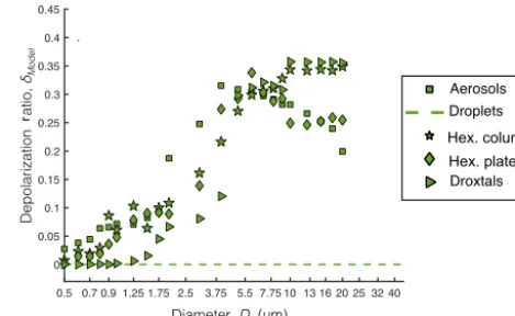
Three idealized ice crystal habits were modeled: a hexag-onal column, a hexaghexag-onal plate, and a droxtal. These shapes represent generalizations of common ice crystal habits (Bai-ley and Hallett, 2009). An idealized dust-like particle with fractal facets was used to model aerosols (Liu et al., 2013). These particles are nonspherical and thus will yield differ-ent measured depolarization ratios depending on their ori-entation in the CASPOL. The model provides the mean de-polarization ratio over all orientations with respect to the laser beam. In contrast, the theoretical depolarization of wa-ter droplets is zero at all sizes.
Figure 2 shows the depolarization ratios as a function of size for the three ice crystal habits, dust-like aerosol, and wa-ter droplets. For hexagonal columns, hexagonal plates, and droxtals, the depolarization ratio increases from less than 0.05 to as high as 0.35 as the optical diameter increases from 0.5 to 8 µm diameter. Above 8 µm, the depolarization ratio for droxtals and columns continue to rise, while the values for plates decrease to∼0.25. The droxtal depolarization ra-tios are quite low. Thus, while columns and plates could be distinguished from water droplets based on depolarization ra-tio alone, droxtals could not be distinctly identified. It is not known which of these habits best represents individual ice crystals nucleated and grown in the CFDC. Fortunately, if it is assumed that only particles of 2 µm diameter or larger are ice crystals in the CFDC, these theoretical results show that discrimination between water droplets and any of the three habits of ice crystals is possible. Thus, consideration of de-polarization ratio should provide a large improvement in par-ticle discrimination.
Similar to ice crystals, depolarization ratios of the mod-eled dust aerosols increase with particle diameter. At most sizes, the aerosol data fall within the range of
depolariza-Hex. columns Hex. plates
r
Figure 2.Depolarization ratio vs. diameter for modeled particles: droplets, aerosols, hexagonal column ice crystals, hexagonal plate ice crystals, and droxtals.
tions ratios reported for the three ice crystal shapes. This in-dicates that the use of depolarization ratios will not make an improvement in differentiating between aerosols and ice crystals. Fortunately, the traditional CFDC method incorpo-rates the use of an impactor to physically remove aerosols greater than 1.75 µm from the sample flow prior to enter-ing the chamber, coupled with the analysis strategy, which only counts particles that are larger than the nominal size cutoff (at least 2 µm diameter) as ice crystals. Thus, the tradi-tional method is already sufficient for differentiating between aerosols and ice crystals.
3.3 Determination of optical properties of aerosols, droplets, and ice crystals
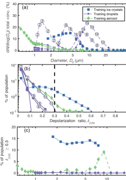
In this section, we empirically test the assertion that the CASPOL depolarization ratio can be used to discriminate ice crystals from aerosols and water droplets. To accomplish this, the training datasets of droplets, aerosols, and ice crys-tals shown above (Fig. 1) are examined further. The lognor-mal size distributions (shown as a percent of population) ob-served by the CASPOL for the droplet, aerosol, and ice crys-tal training data are shown in Fig. 3a. Each VOAG size in the droplet training dataset is treated as a separate popula-tion and plotted as a separate line in the figure. As seen in Fig. 1a, the size distributions of droplets, aerosols, and ice crystals overlap. This demonstrates the primary disadvantage to using particle diameter as the sole criteria to identify ice crystals.
Figure 3. (a)Percent lognormal size distribution,(b)frequency dis-tribution of depolarization ratios, and(c)the percentage of the parti-cles with depolarization ratios above the threshold of 0.3 are shown for training data droplets, aerosols, and ice crystals as detected by the CASPOL. In panel(b), the depolarization ratio threshold value of 0.3 is indicated by the dashed line. In panel (a, b), the num-bers displayed in circles provide the diameter in micrometers of the VOAG data represented by that line.
have depolarizations greater than this threshold. However, since aerosols with sizes above 1.75 µm diameter are physi-cally removed from the sample upstream of the CFDC cham-ber, the combined consideration of size and depolarization may prove a robust strategy for avoiding the miscounting of aerosols as INP as further discussed below.
In Fig. 3c, the percent of particles that achieve a depolar-ization ratio≥0.3 (the nominal selection criteria for depolar-izing ice crystals) as a function of particle diameter is shown. In Fig. 3c, the droplet training data collected for all sizes of olive oil droplets are combined and displayed as one line for simplicity. In contrast to the size distributions (Fig. 3a), in which the training datasets cannot be discriminated, the de-polarization ratio distributions show notable differences be-tween droplets, aerosols, and ice crystals. Figure 3b and c reveal that only 0.3 % of droplets and 1.6 % of aerosol parti-cles achieve a depolarization ratio ≥0.3. The exception to this is aerosols with diameters of 5 to 10 µm. In this size range, 3.9 % of aerosols achieve a depolarization ratio of 0.3.
However, 5 to 10 µm particles are not abundant in nature, cannot easily be sampled by real-time instruments with the inlet complexity of a CFDC, and only represent 0.3 % of the aerosol training dataset. Furthermore, particles in this size range were not generated during the FIN-02 campaign. In contrast, 13.5 % of particles in the ice crystal training dataset achieve a depolarization ratio of at least 0.3. This natural break in the depolarization ratio distributions can be consid-ered as a threshold for which particles above the threshold are ice. Below the threshold, the identity of particles is unknown since the majority of all three populations have depolariza-tion ratios between 0 and 0.3.
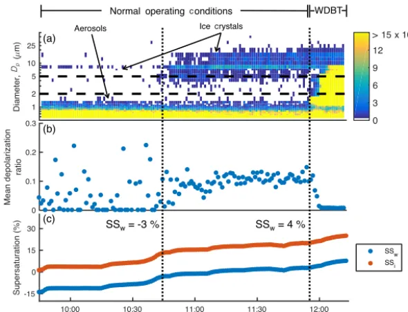
Figure 4. (a)The normalized size distribution,(b)mean depolarization ratio of particles in CFDC with diameter>2 µm, and(c) supersatu-ration conditions with respect to ice (SSi)and water (SSw)for a Snomax®scan on 27 March at−15◦C±1.5◦C (case no. 27 in Table 1). The dashed lines in the figure denote the onset of abundant ice nucleation (10:45) and the onset of WDBT (11:55).
to approximately zero, consistent with the theoretical depo-larization ratio of water droplets. This is similar to the low mean depolarization ratio of training dataset droplets. Taken together, these results show that the mean depolarization ra-tio of particles larger than 2 µm has a strong dependence on whether or not WDBT is occurring in the CFDC. This makes the mean depolarization ratio a useful tool for confirmation of the onset of water droplet breakthrough.
3.5 Optical properties of particles present in the CFDC In this section, the frequency distribution of depolarization ratios of particle populations present in the CFDC are inves-tigated for comparison to the training datasets. First, all data from the FIN-02 campaign were classified as WDBT condi-tions or normal operating condicondi-tions. Then particle diame-ters were used to determine the particle type. Aerosol par-ticles during the FIN-02 campaign were generally smaller than 2 µm in size. Since water droplets can bias this popu-lation during WDBT conditions, only those particles smaller than 2 µm in diameter during normal operating conditions are defined as aerosols. Particles≥2 µm in diameter during nor-mal operating conditions are identified as ice crystals. A third population is defined as “WDBT particles” and consists of particles≥2 µm in diameter during WDBT conditions. This population typically consists of mostly water droplets but can also include ice crystals. These three populations are referred to as “CFDC populations” in this paper.
Figure 5 shows the depolarization ratio distributions of the CFDC populations interpreted to be ice crystals, water
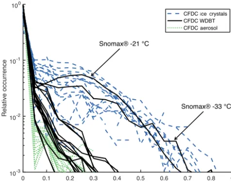
droplets, and aerosols. For the analysis completed to pro-duce Fig. 5, 19 normal operating condition periods and 17 WDBT periods with variable time lengths were classified. Ice crystals achieve higher depolarization ratios than water droplets and aerosol; 13.5 % of ice crystals in the CFDC achieve a depolarization ratio larger than 0.3, compared to 1.5 % percent of water droplets and 0.3 % of aerosols. These values are very similar to the percentages of training data particles that achieve a depolarization ratio greater than 0.3. Ice crystals achieve depolarization ratios larger than 0.3 more than 10 times more frequently than aerosol or water droplets. One interesting feature in the CFDC observations are the two Snomax®cases (cases 13 and 14 in Table 1 at−33 and −21◦C, respectively) in Fig. 5. More particles with high de-polarization ratios were observed than during the other 15 WDBT cases. These particles are most likely ice crystals. Since Snomax®bacteria are a particularly active INP it is not surprising that ice crystals dominate the population of parti-cles in the CFDC even during WDBT (Wex et al., 2015), particularly for runs with lower temperatures.
3.6 Comparing CASPOL observations to model calculations
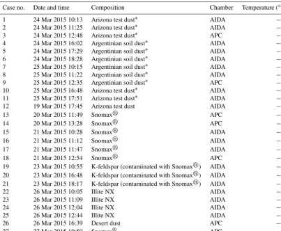
Table 1.Date and time (CET), the composition of aerosol sampled, and the CFDC operating temperature (±1.5◦C).
Case no. Date and time Composition Chamber Temperature (◦C)
1 24 Mar 2015 10:13 Arizona test dust∗ AIDA −25
2 24 Mar 2015 11:25 Arizona test dust∗ AIDA −20
3 24 Mar 2015 12:48 Arizona test dust∗ APC −19
4 24 Mar 2015 16:02 Argentinian soil dust∗ AIDA −19
5 24 Mar 2015 17:29 Argentinian soil dust∗ AIDA −18
6 24 Mar 2015 18:28 Argentinian soil dust∗ AIDA −24
7 25 Mar 2015 10:15 Argentinian soil dust∗ AIDA −25
8 25 Mar 2015 11:22 Argentinian soil dust∗ AIDA −28
9 25 Mar 2015 12:35 Argentinian soil dust∗ APC −28
10 25 Mar 2015 16:48 Arizona test dust∗ AIDA −25
11 25 Mar 2015 17:51 Arizona test dust∗ AIDA −28
12 19 Mar 2015 17:45 Arizona test dust AIDA −34
13 20 Mar 2015 11:49 Snomaxr APC −33
14 20 Mar 2015 13:28 Snomaxr APC −21
15 21 Mar 2015 10:28 Snomaxr AIDA −16
16 21 Mar 2015 11:12 Snomaxr AIDA −19
17 21 Mar 2015 11:47 Snomaxr AIDA −20
18 21 Mar 2015 12:54 Snomaxr APC −15
19 23 Mar 2015 10:55 K-feldspar (contaminated with Snomaxr) AIDA −30
20 23 Mar 2015 16:48 K-feldspar (contaminated with Snomaxr) AIDA −25
21 23 Mar 2015 18:17 K-feldspar (contaminated with Snomaxr) AIDA −21
22 26 Mar 2015 10:05 Illite NX AIDA −25
23 26 Mar 2015 11:09 Illite NX AIDA −25
24 26 Mar 2015 12:04 Illite NX AIDA −28
25 26 Mar 2015 12:44 Illite NX AIDA −30
26 26 Mar 2015 16:39 Desert dust APC −29
27 27 Mar 2015 10:59 Snomax® APC −16
∗Data collected during “blind tests”. Sample composition was provided by the referees after the experiment was completed.
shapes) ice crystals (pentagrams), aerosols (squares), and droplets/WDBT particles (circles). Observed values are ac-companied by error bars representing the standard deviation of depolarization ratios of particles at the respective diame-ters plotted. The CFDC populations presented here include particles sampled from all FIN-02 experiments, and not only those discussed in Sect. 3.5 above. The same conventions are used here to process these particles: CFDC ice crystals are those larger than 2 µm sampled under normal operating con-ditions; CFDC aerosols are those smaller than 2 µm sampled under normal operating conditions; and CFDC WDBT parti-cles are those larger than 2 µm sampled under WDBT condi-tions.
In Fig. 6, both the model calculations and the observed results indicate that ice crystals have higher mean depolar-ization ratios than water droplets and aerosols on average at diameters above 5 µm. However, error bars show that the standard deviations of depolarization ratios at these sizes are very large and that differences in the mean depolarization ra-tios of the observed particles displayed are not statistically significant. This represents a major challenge in designing a
new analysis method that uses depolarization ratio to quan-tify INP.
In Sect. 3.5, the complex WDBT population was dis-cussed. WDBT particles consist of both water droplets and ice crystals. Diffusional growth theory dictates that ice crys-tals will grow to larger sizes in the CFDC than water droplets (Pruppacher and Klett, 2010). Figure 6 shows an increase in the depolarization ratio from ∼0 to 0.25 in the CFDC WDBT population starting at∼6 µm. At diameters greater than 10 µm the mean depolarization ratio of WDBT parti-cles is greater than or equal to the depolarization of CFDC ice crystals and training dataset ice crystals, suggesting that these large particles are mostly or all ice crystals. It is in-ferred that particles in the 6 to 10 µm range are a mixture of water droplets and ice crystals.
Figure 5.Frequency distribution of depolarization ratios for CFDC populations: ice crystal periods (19 periods classified), WDBT pe-riods (17 pepe-riods classified), and aerosol pepe-riods (19 pepe-riods clas-sified). Mean temperatures of periods included range from−15 to −35◦C.
One possible reason for the discrepancies between the model and observations is that the CASPOL depolarization detec-tor underestimates the depolarization of particles due to the weak depolarization of particles and relatively high detection limit of the CASPOL perpendicularly polarized detector. In general, particles scatter relatively little perpendicularly po-larized light in the backward 1 raw count, which translates roughly to a scattering cross section of ∼1×10⁻¹³cm2. This limit results in the CASPOL registering a perpendicular signal below CASPOL’s detection limit for 45 % of training ice crystals, 76 % of training aerosols, and 57 % of training droplets. In the training datasets, all particles with undetected perpendicularly polarized detector were assigned depolariza-tion ratio of zero. Another possibility is that the idealized model particles do not accurately depict the shape, composi-tion, or other microphysical properties of the observed par-ticles. Smith et al. (2016) found that after an ice crystal has nucleated, the geometry of the ice crystal can be modified leading to drastic differences in the observed depolarization ratio. To investigate this, Smith et al. (2016) operated the Manchester Ice Cloud Chamber at different temperatures and supersaturations to produce an assortment of ice crystal mor-phologies including solid and hollow columns, plates, sec-tored plates, and dendrites. During that study, they also com-pared observed and modeled depolarization ratio results and found that on average the difference between modeled and observed depolarization ratios was∼120 %. The CFDC re-sults reported in Fig. 6 include data from all of the runs sam-pled during FIN-02. The dataset of the campaign represents ice nucleation events over a broad range of temperature (−15 to−35◦C) and supersaturation (0 to 40 % SSi)conditions.
Thus, many different habits of ice crystals likely formed in the CFDC, in part, contributing to the wide range of depolar-ization ratios reported in Fig. 6. Nicolet et al. (2007) reported modeling results of single particles that confirm that a wide range of depolarization ratios can be detected for a single shape depending on the orientation. Non-preferential orien-tation of particles in the CFDC is likely to contribute to the breadth of depolarization ratios detected.
The observations are qualitatively consistent with the model in that ice crystals depolarize more light than water droplets and aerosols. However, the discrepancies between the observed and modeled mean depolarization ratios and the wide distributions of observed depolarization ratios dictate that we cannot rely on a mean modeled depolarization ratio to identify and quantify ice crystals in the CFDC. Rather than designing a theoretical model based on model calculations, we move forward by designing an empirical model based on the CASPOL observed signals.
3.7 Designing an empirical model to quantify INP with depolarization ratio
The results above show that counting ice crystals in the CFDC using depolarization ratio can be challenging since only∼13.5 % of ice crystals achieve a depolarization ratio greater than 0.3 (Fig. 3). A depolarization ratio threshold of 0.3 is a favorable criterion to detect ice crystals because less than 2 % of the water droplets and aerosols achieve this de-polarization ratio. However, when there are extreme concen-trations of water droplets, such as those experienced during water droplet breakthrough conditions, the water droplet con-centration may be 103times greater than the ice crystal con-centration in the CFDC, effectively reducing the signal (ice crystals) to noise (water droplets withδ≥0.3) ratio∼1 : 1 or worse. Therefore, an INP concentration cannot be deter-mined by simply applying a depolarization ratio criterion to detect ice crystals with the CFDC-CASPOL.
To obtain a more accurate INP concentration, we used a linear regression model to fit the number of particles with depolarization ratios above the threshold (0.3) to the num-ber of ice crystals in the CFDC. Linear regressions are fre-quently used to interpret the signal(s) of new instrumentation or new techniques by validating the signal with a “ground truth” measurement (e.g., Li et al., 2016; Zimmerman et al., 2017; Brunner et al., 2016; Choi et al., 2016).
Figure 6. Mean depolarization ratios vs. particle diameter for modeled and observed particles. Observed error bars provide a standard deviation on the depolarization ratios of particles at each reported size. No error bars are reported for model calculations.
crystal, and droplet training datasets are randomized in time before particles are selected from each population to cre-ate the simulcre-ated datasets. (This analysis is possible because the data point for each individual particle detected by the CASPOL includes forward scattering, backward scattering, and depolarization).
In total 50 simulated datasets are generated. Table S1 in the Supplement 50 the concentration of ice crystals, water droplets, and aerosols in each dataset. Each simulated dataset is divided into 120 segments, containing a number of ice crystals ranging from 0 to 350. The number of water droplets and aerosols are constant throughout all segments in a single dataset. All 50 datasets contain segments with the same num-ber of randomly selected ice crystals. The upper range ofM values here represents an extreme sampling condition where there are many aerosols and many cloud condensation nuclei that will form cloud droplets, but few INP. Given the rela-tively high number of aerosols and droplets, this would rep-resent the most challenging sampling scenario for proposed new method.
The quantity of aerosols and water droplets in each dataset is determined by a multiplication factorM, such that the number of water droplets=100M and the number of aerosols =300M. For example, the first simulated dataset (M=1) contains 100 water droplets and 300 aerosols. For each iteration,Mis increased by 1. In summary, 50 datasets were generated, containing 100 to 5000 water droplets and 300 to 15 000 aerosol particles.
As discussed above, particles in the INP datasets smaller than the CFDC size cut of 2 µm diameter were removed. Next, for each of the 120 segments in the simulated dataset, the number of particles with a depolarization ratio greater than or equal to a selected depolarization ratio threshold (ranging from 0 to 0.75 in increments of 0.05) is determined. A linear fit is determined for the relationship between the known ice crystal concentration and the number of
parti-0.1 0.2 0.3 0.4 0.5 0.6 0.7 Depolarization ratio threshold 5
10 15 20 25 30 35 40 45 50
R
el
at
iv
e
ae
ro
so
l/d
ro
pl
et
c
on
c.
, M
0.1 0.2 0.3 0.4 0.5 0.6 0.7 0.8 0.9
R
2
al
ue
M
M
ul
tip
lic
at
io
n
fa
ct
or
,
M
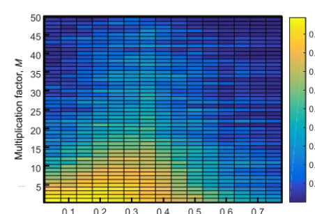
v
Figure 7.R2values for linear regression fit as a function of depolar-ization ratio threshold for optimizing ice crystal differentiation and water droplet and/or aerosol concentration multiplication factor,M.
cles detected greater than or equal to the depolarization ratio threshold for the first dataset (M=1). The linear regression fit is applied to all of the simulated datasets over the entire range ofM. Only one fit is determined for each threshold be-cause we cannot feasibly design a model that adapts to water droplet and aerosol concentration in the CFDC AnR2value is determined to assess the goodness of the linear regression fit over all of the simulated datasets.
de-Figure 8.Application of depolarization ratio method on three CFDC runs. Aerosol composition and temperature are labeled in the title.
(a)Time series of supersaturation with respect to water.(b)INP concentrations under normal (blue) and WDBT (red) conditions are shown for the traditional (circle) and new (asterisk) analysis methods. (c)The normalized number distributions of all particles detected by the CASPOL. Time is reported in local time (CET).
creases. This is especially true for lower depolarization ratio thresholds that are more sensitive to increases in droplets and aerosols. An optimal choice for depolarization ratio thresh-old is defined as a threshthresh-old that retains highR2values across the entire range of M. The threshold should be sufficiently high that it is not sensitive to water droplets and aerosols that may be highly depolarizing and sufficiently low that parti-cles are still detected. Figure 7 shows that a threshold value of 0.35 out performs all other thresholds whenM is larger than 20, including our initial visually chosen threshold value of 0.3. The meanR2value for the 0.35 threshold is 0.46. The next best performing threshold is 0.3 with a meanR2value of 0.44. However, aerosol and water droplet concentrations in CFDC experiments are typically in the range of 1< M <20. The meanR2 value in this range ofMfor the 0.3 and 0.35 thresholds 0.71 and 0.7, respectively. While the performance of these thresholds perform comparably over this range, we selected the 0.3 threshold because it will slightly outperform the 0.35 threshold, especially when detecting lower INP con-centrations.
The linear regression for the 0.3 threshold is provided in Eq. (9):
NINP=6.11Nδ+22.20, (9)
whereNδis the number of particles that have a depolarization
ratio greater than 0.3 and NINP is the derived INP number. Next, Eq. (9) is applied to all CFDC-CASPOL data collected during the FIN-02 campaign and the accuracy of this model is assessed.
104 106 108
Concentration (L-1)
27 26 25 24 23 22 21 20 19 18 17 16 15 14 13 12 11
109
8 7 6 5 4 3 2 1
Ice period (traditional) Ice period (new) WDBT (traditional) WDBT (new)
3.8 Application of the new analysis method to CFDC data collected during FIN-02
INP concentrations were obtained using both the depolar-ization ratio method (Eq. 9) and the traditional method on CFDC data collected during the FIN-02 campaign. Three representative CFDC runs of Snomax® at −15◦C and at −20◦C and Arizona test dust at−25◦C are shown in Fig. 8. Each humidity scan starts in subsaturated conditions with respect to water. Supersaturation is gradually increased un-til ice nucleation initiates and then further increased unun-til WDBT occurs (represented by the red symbols in Fig. 8). The reported concentrations reveal that the traditional (cir-cles) and depolarization ratio (*) methods generally agree during “ice-only” periods (blue symbols in Fig. 8). In most cases there is clear disagreement between concentrations in WDBT periods, for example in the cases of Snomax® at −15◦C and Arizona test dust at−25◦C. This is expected
since the traditional concentration is sensitive to an increase in water droplets that grow larger than the size cut applied in WDBT conditions, where INP concentrations are usually not reported. An exception to this can be seen in Fig. 8b, the Snomax® at −20◦C. The concentrations from the two methods remain in good agreement as the supersaturation is increased into the WDBT period. In this case, the ice crystal concentration is dominating the population in WDBT. The evidence for this is the high concentration of ice crystals that from 13:15 CET as observed in the size distribution time se-ries in center panel Fig. 8b.
Figure 9 summarizes the mean concentrations obtained through the traditional and new method for all periods when the CFDC was operational during FIN-02. In total, 27 ice-only periods and WDBT cases are included. A description of the date and time, aerosol composition, and temperature of each case is detailed in Table 1. In cases 24, 25, and 26 WDBT did not occur, so no data are reported. The error bars report the CFDC-CASPOL uncertainty in INP concentration, which is 39 % based on combined instrumental uncertainties (Glen and Brooks, 2014, 2013), Fig. 9 shows that in all but 4 cases out of 27 (cases 2, 7, 9, and 23), the mean concen-tration of the new analysis method is in agreement with tra-ditional analysis method for the ice-only periods. Figure 9 also shows that only 9 out of 24 WDBT cases have statistical agreement between the new and traditional analysis method. At the onset of WDBT, the impact of water droplets on the INP concentration determined by the 2 µm size cut may not be very large and the concentration may closely resemble the true INP concentration, but as the SSwis increased more wa-ter droplets will be incorrectly counted in the traditional INP concentration. This phenomenon gives rise to the large error bars reported in some of the WDBT cases. In general, the ob-servations reported in Fig. 9 are consistent with the assertion that the traditional method and new method are in agreement during the ice-only periods and that during WDBT the tradi-tional method is elevated in response to large water droplets
Figure 10.Traditional INP concentration vs. new INP concentra-tion with 1 : 1 line for “ice-only” periods.
miscounted as INP while the depolarization ratio method re-mains accurate.
To summarize the comparison between our new method and the traditional method during the ice-only periods, the INP concentrations determined using the traditional method vs. new method are plotted in Fig. 10. Each point on the plot represents data for a 1 min segment. The black line in Fig. 10 is a 1 : 1 line. Since the analysis used to generate Fig. 10 only uses data collected under normal operating conditions (not WDBT), the traditional concentration can be considered ground truth. The data closely follow the 1 : 1 line, confirm-ing that the depolarization ratio can be used to reliably re-trieve an INP concentration when no or few water droplets and/or aerosols are larger than 2 µm. To assess the perfor-mance of the new method we use mean percent error (MPE) defined here as
MPE=new concentration−traditonal concentration
traditional concentration ×100 %. (10)
The MPE of the method is dependent on the INP concen-tration. Due to the high detection limit of concentration for the CASPOL, the MPE of the new method is±500 % when the traditional concentration is between 0 and 50 000 L−1. However, at higher concentrations the MPE is typically ±50 % or less. Additionally, Fig. 10 shows that at concentra-tions in the range of 0 to 3×10⁶L−1, the new method typ-ically undercounts INPs but overcounts INPs at higher con-centrations (greater than 3×10⁶L−1). The MPE for the new method for all concentrations is±32.1 %.
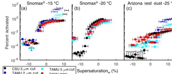
Figure 11.TAMU CFDC versus CSU CFDC comparison:(a)Snomax®at−15◦C,(b)Snomax®at−20◦C, and(c)Arizona test dust at −25◦C. Small symbols indicate that those points were sampled in WDBT. TAMU 2 µm cut and 5 µm cut traditional activated INP fraction are shown in blue and cyan, respectively. The TAMU new analysis method activated INP fraction is shown in red. The CSU 3 µm INP fraction activated is shown in black.
100 L−1(e.g., Mason et al., 2016; Jiang et al., 2014; DeMott et al., 2003; Kanji et al., 2017). Nonetheless, the new method is considered an improvement for use during water droplet breakthrough, when the traditional method cannot be used.
As a final test of the new method during water droplet breakthrough periods, a reliable measure of INP at higher supersaturation conditions (when the TAMU CFDC is ex-periencing WDBT) is needed. Due to design and flow rate differences, the CSU CFDC does not experience the onset of WDBT until higher supersaturations than the TAMU CFDC, up to 108 % or higher depending on temperature (DeMott et al., 2015). Thus, inclusion of the CSU data provides a test of the new method at higher relative humidities under condi-tions when data obtained through the TAMU CFDC’s tradi-tional method is spurious due to water droplet breakthrough. Figure 11 shows the comparison of the TAMU CFDC’s tra-ditional (2 µm size cut) and new method INP concentrations and the CSU CFDC INP concentration, collected during the FIN-02 campaign. Because CASPOL sizing of nonspherical ice crystals nucleated and grown in the chamber is uncer-tain, the data were also analyzed using a 5 µm size cut to provide an estimate of the lower limit of INP concentration. As discussed above, the CSU CFDC has a longer chamber, a different evaporation region design, a different detector, and a chosen size cut of 3 µm. Results of INP percent activated are reported from three CFDC runs discussed earlier includ-ing Snomax® at−15 and −20◦C and Arizona test dust at −25◦C. Concentrations used to calculate the percent activa-tion are average concentraactiva-tions of samples in a 1 % range of SSw conditions in the CFDC. Large symbols show data collected under normal operating conditions. Small symbols show data collected during WDBT conditions in the TAMU CFDC. The CSU CFDC did not experience WDBT in the data reported in Fig. 11. The traditional concentration from TAMU and CSU and the new method concentration all are in reasonable agreement during ice-only conditions for all three cases. During WDBT, the TAMU traditional
concen-trations increase in response to the water droplets that grow larger than the size criteria (2 or 5 µm). Fortunately, the new method remains in agreement with the CSU concentration. Figure 11b shows the special case of high activation of INP shown in Fig. 8b. This case involves a highly active INP, Snomax®at−20◦C, a significantly colder temperature than required for the Snomax®to activate as INP. Since most par-ticles activated prior to the onset of WDBT, there is negligi-ble difference in the concentrations reported during ice-only and WDBT periods. In conclusion, the new method accu-rately determines the INP concentration in the presence of water droplets and can thus extend the range of operating conditions of the TAMU CFDC.
4 Conclusions
For this reason, the new CASPOL depolarization method is recommended for CFDC laboratory experiments only. A comparison between the CSU CFDC INP concentration and TAMU CFDC INP concentration derived from the new anal-ysis method show agreement even under conditions in which the TAMU CFDC experiences WDBT and CSU does not experience WDBT. We conclude that the new method can be used to extend the range of operating conditions in the CFDC. However, under conditions encountered in field stud-ies, the traditional method is still preferred analysis method for counting ice nucleating crystals with the TAMU CFDC.
Data availability. The data used in this study will be made
avail-able in a future publication (DeMott et al., 2017).
The Supplement related to this article is available online at https://doi.org/10.5194/amt-10-4639-2017-supplement.
Competing interests. The authors declare that they have no conflict
of interest.
Acknowledgements. The authors acknowledge primary support
from the National Science Foundation, grant no. ECS-1309854. Ezra J. T. Levin, Kaitlyn J. Suski, and Paul J. DeMott acknowledge support from NSF grant no. AGS-1358495. The FIN-02 and FIN-03 campaigns were supported by NSF grant no. AGS-1339264 and by the US Department of Energy’s Atmospheric System Research, an Office of Science, Office of Biological and Environmental Research program, under grant no. DE-SC0014487. Special thanks to Daniel Cziczo and Ottmar Möhler for their roles in coordinating the FIN-02 and FIN-03 studies and to all research teams involved in making those studies possible.
Edited by: Mingjin Tang
Reviewed by: four anonymous referees
References
Amato, P., Joly, M., Schaupp, C., Attard, E., Möhler, O., Morris, C. E., Brunet, Y., and Delort, A.-M.: Survival and ice nucleation activity of bacteria as aerosols in a cloud simulation chamber, At-mos. Chem. Phys., 15, 6455–6465, https://doi.org/10.5194/acp-15-6455-2015, 2015.
Atkinson, J. D., Murray, B. J., Woodhouse, M. T., Whale, T. F., Baustian, K. J., Carslaw K. S., Dobbie S., O’Sullivan, D., and Malkin, T. L.: The importance of feldspar for ice nucleation by mineral dust in mixed-phase clouds, Nature, 498, 355–358, 2013. Bailey, M. P. and Hallett, J.: A comprehensive habit diagram for at-mospheric ice crystals: Confirmation from the laboratory, AIRS II, and other field studies, J. Atmos. Sci., 66, 2888–2899, 2009.
Bi, L. and Yang, P.: Accurate simulation of the optical properties of atmospheric ice crystals with the invariant imbedding T-matrix method, J. Quant. Spectrosc. Ra., 138, 17–35, 2014.
Bi, L., Yang, P., Kattawar, G. W., and Mishchenko, M. I.: Efficient implementation of the invariant imbedding T-matrix method and the separation of variables method applied to large nonspheri-cal inhomogeneous particles, J. Quant. Spectrosc. Ra., 116, 169– 183, 2013.
Bohren, C. F. and Huffman, D. R.: Absorption and Scattering of Light by Small Particles, Wiley-VCH, Weinheim, Germany, 1983.
Boucher, O., Randall, D., Artaxo, P., Bretherton, C., Feingold, G., Forster, P., Kerminen, V. M., Kondo, Y., Liao, H., Lohmann, U., and Rasch, P.: Clouds and Aerosols, in: Climate Change: The Physical Science Basis. Contribution of Working Group I to the Fifth Assessment Report of the Intergovernmental Panel on Cli-mate Change, Cambridge University Press, Cambridge, UK and New York, NY, USA, 571–657, 2013.
Brooks, S. D., Toon, O. B., Tolbert, M. A., Baumgardner, D., Gan-drud B. W., Browell E. V., Flentje, H., and Wilson, J. C.:, Polar stratospheric clouds during SOLVE/THESEO: Comparison of li-dar observations with in situ measurements, J. Geophys. Res.-Atmos., 109, D02212, https://doi.org/10.1029/2003JD003463, 2004.
Brooks, S. D., Suter, K., and Olivarez, L.: Effects of chemical aging on the ice nucleation activity of soot and polycyclic aromatic hy-drocarbon aerosols, J. Phys. Chem. A, 118, 10036–10047, 2014. Brunner, J., Pierce, R. B., and Lenzen, A.: Development and validation of satellite-based estimates of surface visibility, At-mos. Meas. Tech., 9, 409–422, https://doi.org/10.5194/amt-9-409-2016, 2016.
Choi, M., Kim, J., Lee, J., Kim, M., Park, Y.-J., Jeong, U., Kim, W., Hong, H., Holben, B., Eck, T. F., Song, C. H., Lim, J.-H., and Song, C.-K.: GOCI Yonsei Aerosol Retrieval (YAER) algorithm and validation during the DRAGON-NE Asia 2012 campaign, Atmos. Meas. Tech., 9, 1377–1398, https://doi.org/10.5194/amt-9-1377-2016, 2016.
Clauss, T., Kiselev, A., Hartmann, S., Augustin, S., Pfeifer, S., Nie-dermeier, D., Wex, H., and Stratmann, F.: Application of lin-ear polarized light for the discrimination of frozen and liquid droplets in ice nucleation experiments, Atmos. Meas. Tech., 6, 1041–1052, https://doi.org/10.5194/amt-6-1041-2013, 2013. Collier, K. N. and Brooks, S. D.: Role of organic hydrocarbons in
atmospheric ice formation via contact freezing, J. Phys. Chem. A, 120, 10169–10180, 2016.
Coluzza, I., Creamean, J., Rossi, M. J., Wex, H., Alpert, P. A., Bianco, V., Boose, Y., Dellago, C., Felgitsch, L., Fröhlich-Nowoisky, J., Herrmann, H., Jungblut, S., Kanji, Z. A., Menzl, G., Moffett, B., Moritz, C., Mutzel, A., Pöschl, U., Schau-perl, M., Scheel, J., Stopelli, E., Stratmann, F., Grothe, H., and Schmale III, D.: Perspectives on the Future of Ice Nucleation Research: Research Needs and Unanswered Questions Identi-fied from Two International Workshops, Atmosphere, 8, 138, https://doi.org/10.3390/atmos8080138, 2017.
Cziczo, D. J., Ladino, L., Boose, Y., Kanji, Z. A., Kupiszewski, P., Lance, S., Mertes, S., and Wex, H.: Measurements of Ice Nu-cleating Particles and Ice Residuals, Meteor. Mon., 58, 8.1–8.13, 2017.
De Boer, G., Morrison, H., Shupe, M., and Hildner, R.: Evidence of liquid dependent ice nucleation in high-latitude stratiform clouds from surface remote sensors, Geophys. Res. Lett., 38, L01803, https://doi.org/10.1029/2010GL046016, 2011.
DeMott, P. J., Sassen, K., Poellot, M.R., Baumgardner, D., Rogers, D. C., Brooks, S. D., Prenni, A. J., and Kreidenweis, S. M.: African dust aerosols as atmospheric ice nuclei, Geophys. Res. Lett., 30, 1732, https://doi.org/10.1029/2003GL017410, 2003. DeMott, P. J., Möhler, O., Stetzer, O., Vali, G., Levin, Z.,
Pet-ters, M. D., Murakam, M., Leisner, T., Bundke, U., Klein, H., Kanji, Z., Cotton, R., Jones, H., Petters, M., Prenni, A., Benz, S., Brinkmann, M., Rzesanke, D., Saathoff, H., Nicolet, M., Gallavardin, S., Saito, A., Nillius, B., Bingemer, H., Abbatt, J., Ardon, K., Ganor, E., Georgakopoulos, D. G., and Saunders, C.: Resurgence in ice nucleation research, B. Am. Meteorol. Soc., 92, 1623–1635, 2011.
DeMott, P. J., Prenni, A. J., McMeeking, G. R., Sullivan, R. C., Petters, M. D., Tobo, Y., Niemand, M., Möhler, O., Snider, J. R., Wang, Z., and Kreidenweis, S. M.: Integrating laboratory and field data to quantify the immersion freezing ice nucleation activ-ity of mineral dust particles, Atmos. Chem. Phys., 15, 393–409, https://doi.org/10.5194/acp-15-393-2015, 2015.
DeMott, P. J., Hill, T. C., McCluskey, C. S., Prather, K. A., Collins, D. B., Sullivan, R. C., Ruppel, M. J., Mason, R. H., Irish, V. E., and Lee, T.: Sea spray aerosol as a unique source of ice nucleat-ing particles, P. Natl. Acad. Sci. USA, 113, 5797–5803, 2016. DeMott, P. J., et al.: Overview of results from the Fifth
Interna-tional Workshop on Ice Nucleation, Part 2 (FIN-02): Laboratory intercomparisons of ice nucleation measurements, Atmos. Chem. Phys. Discuss., in preparation, 2017.
Durant, A. J. and Shaw, R. A.: Evaporation freezing by con-tact nucleation inside-out, Geophys. Res. Lett., 32, L20814, https://doi.org/10.1029/2005GL024175, 2005.
Fornea, A. P., Brooks, S. D., Dooley, J. B., and Saha, A.: Het-erogeneous freezing of ice on atmospheric aerosols contain-ing ash, soot, and soil, J. Geophys. Res.-Atmos., 114, D13201, https://doi.org/10.1029/2009JD011958, 2009.
Garimella, S., Kristensen, T. B., Ignatius, K., Welti, A., Voigtlän-der, J., Kulkarni, G. R., Sagan, F., Kok, G. L., Dorsey, J., Nich-man, L., Rothenberg, D. A., Rösch, M., Kirchgäßner, A. C. R., Ladkin, R., Wex, H., Wilson, T. W., Ladino, L. A., Abbatt, J. P. D., Stetzer, O., Lohmann, U., Stratmann, F., and Cziczo, D. J.: The SPectrometer for Ice Nuclei (SPIN): an instrument to investigate ice nucleation, Atmos. Meas. Tech., 9, 2781–2795, https://doi.org/10.5194/amt-9-2781-2016, 2016.
Glen, A.: The development of measurement techniques to identify and characterize dusts and ice nuclei in the atmosphere, Diss., Texas A&M University, 2014.
Glen, A. and Brooks, S. D.: A new method for measur-ing optical scattermeasur-ing properties of atmospherically relevant dusts using the Cloud and Aerosol Spectrometer with Po-larization (CASPOL), Atmos. Chem. Phys., 13, 1345–1356, https://doi.org/10.5194/acp-13-1345-2013, 2013.
Glen, A. and Brooks, S. D.: Single particle measurements of the optical properties of small ice crystals and heterogeneous ice nu-clei, Aerosol Sci. Tech., 48, 1123–1132, 2014.
Hecht, E. and Zajac, A.: Optics 4th (International) edition, Addison Wesley Publishing Company, 2002.
Hoose, C. and Möhler, O.: Heterogeneous ice nucleation on atmospheric aerosols: a review of results from labo-ratory experiments, Atmos. Chem. Phys., 12, 9817–9854, https://doi.org/10.5194/acp-12-9817-2012, 2012.
Hu, Y., Winker, D., Vaughan, M., Lin, B., Omar, A., Trepte, C., Flittner, D., Yang, P., Nasiri, S. L., and Baum, B.: CALIPSO/CALIOP cloud phase discrimination algorithm, J. At-mos. Ocean Tech., 26, 2293–2309, 2009.
Jiang, H., Yin, Y., Yang, L., Yang, S., Su, H., and Chen, K.: The characteristics of atmospheric ice nuclei measured at different altitudes in the Huangshan Mountains in Southeast China, Adv. Atmos. Sci., 31, 396–406, 2014.
Johnson, B. R.: Invariant imbedding T matrix approach to electro-magnetic scattering, Appl. Optics, 27, 4861–4873, 1988. Kanji, Z. A., Ladino, L., Wex, H., Boose, Y., Burkert-Kohn, M.,
Cziczo, D. J., and Krämer, M.: Overview of Ice Nucleating Par-ticles, Meteor. Mon., 58, 1.1–1.33, 2017.
Koepke, P., Gasteiger, J., and Hess, M.: Technical Note: Optical properties of desert aerosol with non-spherical mineral parti-cles: data incorporated to OPAC, Atmos. Chem. Phys., 15, 5947– 5956, https://doi.org/10.5194/acp-15-5947-2015, 2015. Korolev, A.: Limitations of the Wegener–Bergeron–Findeisen
mechanism in the evolution of mixed-phase clouds, J. Atmos. Sci., 64, 3372–3375, 2007.
Levin, E., McMeeking, G., DeMott, P., McCluskey, C., Carrico, C., Nakao, S., Jayarathne, T., Stone, E., Stockwell, C., and Yokelson, R.: Ice-nucleating particle emissions from biomass combustion and the potential importance of soot aerosol, J. Geophys. Res.-Atmos., 121, 5888–5903, 2016.
Li, S., Joseph, E., and Min, Q.: Remote sensing of ground-level PM2.5combining AOD and backscattering profile, Remote Sens. Environ., 183, 120–128, 2016.
Linke, C., Möhler, O., Veres, A., Mohácsi, Á., Bozóki, Z., Sz-abó, G., and Schnaiter, M.: Optical properties and miner-alogical composition of different Saharan mineral dust sam-ples: a laboratory study, Atmos. Chem. Phys., 6, 3315–3323, https://doi.org/10.5194/acp-6-3315-2006, 2006.
Liu, C., Panetta, R. L., Yang, P., Macke, A., and Baran, A. J.: Mod-eling the scattering properties of mineral aerosols using concave fractal polyhedra, Appl. Optics, 52, 640–652, 2013.
Mason, R. H., Si, M., Chou, C., Irish, V. E., Dickie, R., Elizondo, P., Wong, R., Brintnell, M., Elsasser, M., Lassar, W. M., Pierce, K. M., Leaitch, W. R., MacDonald, A. M., Platt, A., Toom-Sauntry, D., Sarda-Estève, R., Schiller, C. L., Suski, K. J., Hill, T. C. J., Abbatt, J. P. D., Huffman, J. A., DeMott, P. J., and Bertram, A. K.: Size-resolved measurements of ice-nucleating particles at six locations in North America and one in Europe, At-mos. Chem. Phys., 16, 1637–1651, https://doi.org/10.5194/acp-16-1637-2016, 2016.