Non-adiabatic effects
A. V. Artemyev1,2, A. I. Neishtadt1,3, and L. M. Zelenyi1
1Space Research Institute RAS, Profsouznaya st., 84/32, GSP-7, 117997 Moscow, Russia
2Laboratoire de physique et chimie de l’environnement et de l’Espace (LPC2E), UMR7328, CNRS – University of Orleans,
Orleans, France
3Department of Mathematical Sciences, Loughborough University, Loughborough LE11 3TU, UK
Correspondence to: A. V. Artemyev ([email protected])
Received: 4 July 2013 – Revised: 12 September 2013 – Accepted: 20 September 2013 – Published: 31 October 2013
Abstract. We investigate dynamics of charged particles in current sheets with the sheared magnetic field. In our pre-vious paper (Artemyev et al., 2013) we studied the particle motion in such magnetic field configurations on the basis of the adiabatic theory and conservation of the quasi-adiabatic invariant. In this paper we concentrate on violation of the adiabaticity due to jumps of this invariant and the cor-responding effects of stochastization of a particle motion. We compare effects of geometrical and dynamical jumps, which occur due to the presence of the separatrix in the phase plane of charged particle motion. We show that due to the presence of the magnetic field shear, the average value of dynamical jumps is not equal to zero. This effect results in the decrease of the time interval necessary for stochastization of trapped particle motion. We investigate also the effect of the mag-netic field shear on transient trajectories, which cross the cur-rent sheet boundaries. Presence of the magnetic field shear leads to the asymmetry of reflection and transition of parti-cles in the current sheet. We discuss the possible influence of single-particle effects revealed in this paper on the current sheet structure and dynamics.
1 Introduction
Current sheets (CSs) represent one of the most important and intriguing plasma objects in space plasmas. CSs have been studied and observed in planetary magnetospheres (Baumjo-hann et al., 2007; Artemyev and Zelenyi, 2013) and the solar corona (see Syrovatskii, 1979; Parker, 1994, and references therein). Theory of formation and stability of CSs is based
on the detailed description of a charged particle motion (see Whipple et al., 1984; Sitnov et al., 2000; Zelenyi et al., 2000, 2011). The motion of charged particles in inhomogeneous magnetic fields of CSs can be described analytically in two different classes of systems. When a spatial scale of the mag-netic field inhomogeneity is much larger than a particle’s Lar-mor radius, the classical theory of the guiding-centre motion can be applied (Northrop, 1963; Sivukhin, 1965). Another class contains systems where a spatial scale of the magnetic field inhomogeneity is much smaller than a particle’s Larmor radius. In this case the so-called theory of the quasi-adiabatic motion is used (Büchner and Zelenyi, 1986; Büchner and Zelenyi, 1989; Chen, 1992; Vainchtein et al., 2005; Zelenyi et al., 2013).
of adiabaticity results in stochastization of particle motion (Chen and Palmadesso, 1986; Büchner and Zelenyi, 1989; Burkhart and Chen, 1991; Büchner, 1991; Burkhart et al., 1995). These effects are important for particle acceleration in the CSs of the solar corona (Litvinenko, 2003; Anas-tasiadis et al., 2008) and in planetary magnetotails (Büchner and Zelenyi, 1990; Ashour-Abdalla et al., 1992; Cheng and Decker, 1992; Ashour-Abdalla et al., 1994; Delcourt et al., 2003; Grigorenko et al., 2011; Zhou et al., 2012; Zelenyi et al., 2013). Isotropization of particle velocity distribution due to stochastization of particle motion influences the CS configuration in the vicinity of the reconnection region (Le et al., 2013). Moreover, the same effect of the destruction of quasi-adiabatic invariants can play a significant role in parti-cle transport in radiation belts (see Ukhorskiy et al., 2011, and references therein) and in dynamics of the laboratory plasma (e.g. Chirikov, 1979; Carati et al., 2012).
For the simple model of CS without a shear component of the magnetic field,By (here and in the following we use
the GSM coordinate system), the theory of jumps of the quasi-adiabatic invariant is described in details by Büchner and Zelenyi (1989). However, the By component is often
present in the Earth’s magnetotail (see Petrukovich, 2011, and references therein) and in CSs of the solar corona (e.g. Masuda et al., 2001; Schrijver, 2009). This component can affect particle acceleration (Litvinenko, 1996), CS struc-ture (Whipple et al., 1984; Roth et al., 1996; Artemyev, 2011; Malova et al., 2012) and CS dynamics (Galeev et al., 1986; Kuznetsova and Roth, 1995; Silin and Büchner, 2003; Karimabadi et al., 2005; Artemyev and Zimovets, 2012). The influence ofByon particle motion has been studied in several
papers with the help of numerical modelling of test trajecto-ries (Karimabadi et al., 1990; Büchner and Zelenyi, 1991; Zhu and Parks, 1993; Baek et al., 1995; Chapman and Row-lands, 1998; Delcourt et al., 2000). It was noticed thatBy
dramatically influences particle scattering due to jumps of the quasi-adiabatic invariant (Büchner and Zelenyi, 1991; Kauf-mann et al., 1994; Holland et al., 1996). However, no analyt-ical theory of this scattering has been developed so far.
In our previous paper we presented the analytical theory of the quasi-adiabatic particle motion in the CS with an arbi-trary value ofBy(Artemyev et al., 2013). It was shown that
dynamics of particles in the CS withBy6=0 are substantially
more complicated than particle dynamics in non-sheared
tosphere (see review by Paschmann et al., 2002).
The first part of the present paper is devoted toBy
influ-ence on particle interaction with the CS. We consider reflec-tion and transireflec-tion of particles coming to the CS from the CS boundaries. The influence ofBy on particle scattering in
the CS and corresponding stochastization of particle motion is studied in the second part of the present paper, where we concentrate on the investigation of the violation of the adia-baticity.
2 General equations
We study dynamics of particles in the plasma configuration with the sheared magnetic field reversal. This configuration can be represented by the system with the magnetic field
B=Bx(z)ex+Byey+Bzez, whereBz>0 andBy>0 are
constant. Such a model allows also for the CS boundaries to be taken into account:Bx=B0(z/L)at|z/L|<1 andBx= ±B0at|z/L|>1. In the CS central region (where|z/L|<1) the vector potential isA=Byzex+(Bzx−B0z2/2L)ey. The
system is homogeneous along theyaxis, and the correspond-ing canonical momentum, py, is conserved. Thus, we can
shift the coordinate system alongx to set py=0. Due to
stationarity of the magnetic field the energy of each particle is conserved,h=const. The Hamiltonian of a particle with massmand chargeqin this system has the form
H=1
2p
2
z+
1
2(px−sz)
2+1
2(κx− 1 2z
2)2, (1)
where we use dimensionless variables and parameters:H→
H /2h, p→p/
√
2hm, r→r/√ρ0L, dimensionless time
t→t√2h/(ρ0Lm), and parameters κ=(Bz/B0) √
L/ρ0
ands=(By/B0) √
L/ρ0 (ρ0= √
2hmc/(qB0)is a Larmor radius). This normalization corresponds to particle motion in the 3-D energy level H (z, pz, κx, px)=1/2 of 4-D phase
space (z, pz, κx, px). We assume that the parameter κ is
small (κ∈ [0.01,0.1] for energetic and thermal ions in the Earth’s magnetotail CS (see review by Zelenyi et al., 2011, and references therein)). Therefore, variables(κx, px)could
be considered as slow ones, and variables(z, pz)as fast. In
this paper we consider only systems with s > (π−1ln 2)κ
when effects of non-zeroByare well distinguished. For
the plane(κx, px)the particle oscillates in the effective
po-tentialU (z)=1
2(px−sz)2+12(κx− 1
2z2)2at the energy level H=1/2 (see details in Artemyev et al., 2013). The corre-sponding trajectory in the plane(z, pz)can be located inside
the separatrix loops (e.g. Fig. 1a) or outside the separatrix loops (e.g. Fig. 1e). Motion inside the separatrix loops cor-responds to particle oscillations in one of the two small po-tential wells described by popo-tentialU (z). Motion outside the separatrix loops corresponds to either (1) merging of the two small potential wells into a single well, and particle oscil-lations within this newly formed well; or to (2) osciloscil-lations above the two small wells in the potentialU (z)(see details in Artemyev et al., 2013). When the particle crosses the sep-aratrix in the plane(z, pz), it crosses the uncertainty curve
(Wisdom, 1985) in the plane(κx, px)(this curve is shown as
a black solid curve in Fig. 1, top-right panel).
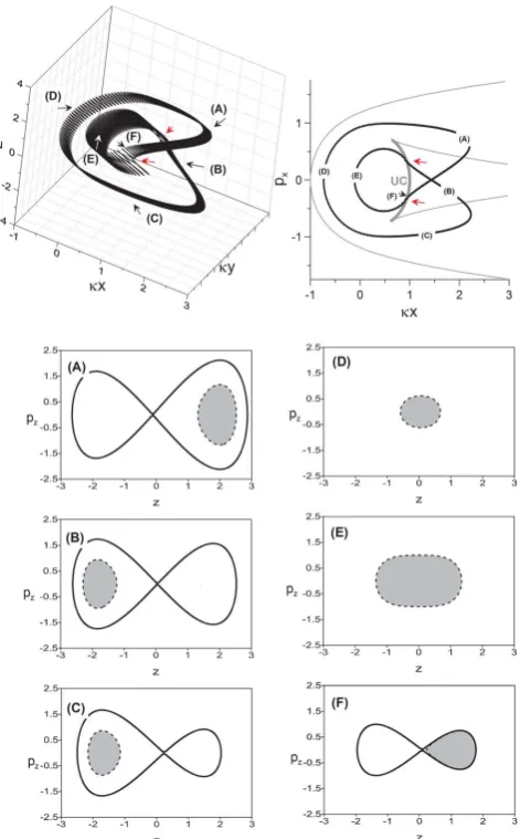
We start the description of the particle trajectory at the point (A). At this point the particle oscillates inside the right potential well far from the separatrix (Fig. 1a) and moves along the field line towards the neutral planez=0. At the point (F) the particle trajectory in the(z, pz)plane
approaches the separatrix (Fig. 1f). Then the particle crosses the separatrix and comes to the point (E). At this point the particle oscillates across the neutral plane, i.e. the trajectory in the(z, pz)plane crossesz=0 (Fig. 1e). Then the
parti-cle crosses the separatrix again and becomes trapped in the left potential well (Fig. 1b and c). Inside this well the particle approaches the neutral plane without crossing of the uncer-tainty curve (Fig. 1d). We emphasize that the particle turns over the uncertainty curve and comes to the neutral plane without crossing of the separatrix. Comparison of panels (d) and (e) shows the difference of two fragments of the particle trajectory. If the particle crosses the separatrix, it starts oscil-lating across the neutral plane with about double amplitude of z. If the particle comes to the neutral plane z=0 with-out crossing the separatrix, it continues oscillating across the field line, which crosses the neutral plane. As a result, am-plitude of particle oscillations is approximately two times smaller in the second case (compare panels (e) and (d)).
At fixed values(κx, px)the trajectory in the(z, pz)plane
is closed, i.e. motion in the plane (z, pz) is periodic (see
Fig. 1a–f). Thus, we can introduce the invariant of motion
Iz=(1/2π )
H
pzdz(Landau and Lifshitz, 1960). This
invari-ant is often called quasi-adiabatic, in contrast to the classi-cal adiabatic invariant represented by the magnetic moment
Fig. 1. The particle trajectory in 3-D space and its projection onto the plane(κx, px)are shown in top panels. Red arrows show
po-sitions of the uncertainty curve (UC) crossings. The corresponding fragments of the particle trajectory in the plane(z, pz)are presented
in the bottom panels. The solid curve is the separatrix, while the dashed curve is the trajectory. Grey colour indicates the area, which is equal to 2π Iz.
(Büchner and Zelenyi, 1986; Büchner and Zelenyi, 1989). Conservation of this invariant is provided by the separation of timescales of evolution ofzandκx. For constant energy (H=1/2) the equation Iz(κx, px)=const describes
parti-cle trajectories in the plane(κx, px)(Büchner and Zelenyi,
1986). However, this equation can be violated when particle trajectories cross the separatrix in the plane(z, pz)
is well defined by the equationIz(κx, px)=const, while a
position of crossing of the separatrix in the plane(z, pz)can
be considered as random because the oscillations of(z, pz)
are fast (i.e. even a small∼κchange of initial coordinates in the plane(z, pz)can change the position of separatrix
cross-ing and the value of the dynamical jump very substantially). Thus, the dynamical jump is assumed to be a quasi-random variable. The geometrical jump does not depend onκ, and is well prescribed (it depends only on position of crossing of the uncertainty curve in the plane(κx, px)). Particle
dynam-ics with effects of the geometrical jumps were considered by Artemyev et al. (2013). In the present paper (in Sect. 4) we describe effects of dynamical jumps and corresponding vio-lation of the adiabaticity of particle motion.
In the previous paper (Artemyev et al., 2013) we consid-ered the system with Hamiltonian (1). However, the presence of the CS boundaries was not taken into account. It is appro-priate as particle trajectories do not cross the planesz= ±λ, whereλ=√L/ρ0. In the present paper (in Sect. 3) we con-sider effects of the boundaries on the particle motion.
It was shown in Artemyev et al. (2013) that, ifs6=0, the particle trajectories can have two options for possible prolon-gations in the plane(κx, px)after crossing of the uncertainty
curve. Thus, there is a splitting of the adiabatic (Iz=const)
trajectories with certain probabilities of various prolonga-tions. We describe details of this effect in Sect. 5.
3 The boundaries of the current sheet
The CS boundaries are located at z= ±L (in the dimen-sionless variablesz= ±λ, whereλ=√L/ρ0). Beyond these boundaries (|z|> λ) the value of theBx component of the
magnetic field is constant,Bx= ±B0. Thus, once particles
reach these boundaries, they escape from the CS. In this section we describe particle motion in the CS including the boundaries. We assume that the crossing of the bound-aries|z| =λoccurs when a particle moving from the region
|z|< λcrosses them. A particle crosses the boundaries when its trajectory (calculated at fixed(κx, px)) in the(z, pz)plane
is located at the space domain|z|> λentirely. Thus, we do not take into account situations when only a fragment of a trajectory is located in the domain|z|> λ. In this considera-tion we also neglect small random (dynamical) jumps ofIz,
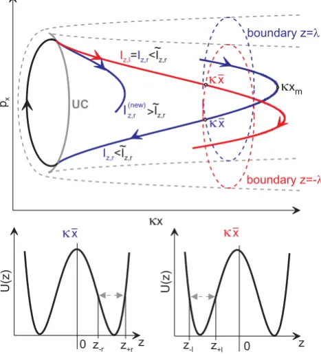
reflected from the CS and reach the opposite boundaryz=λ. The third scenario corresponds to particles initially trapped in the CS. We show how the positions of reflection points of these particles can be changed due to geometrical jumps of
Iz, resulting in escape of particles from the CS. These are
three typical scenarios, i.e. each complex particle trajectory can be considered as a combination of trajectories described by these scenarios.
All these scenarios are characteristic for trajectories in the system withs <0.35. Fors∈(0.35,1)the reflection from the CS is impossible: all particles from the upper boundary
z=λ pass through the CS (with or without a half-rotation aroundBz) and all particles from the bottom boundary z= −λcross the CS without making turns aroundBz (see
de-scription of such trajectories in Artemyev et al., 2013). The general description of particle motion in the system without dynamical jumps ofIzis based on consideration of
adiabatic trajectories in the plane(κx, px). These
trajecto-ries are determined by the equationIz(κx, px)=const. Due
to conservation of the particle energy, each point in the plane
(κx, px) corresponds to a certain closed trajectory in the
plane (z, pz). As a result, if we know all possible particle
positions in the plane(κx, px)for a given value of Iz, we
can predict whether this particle crosses the boundaries. 3.1 The first scenario
We consider a particle that approaches the neutral plane be-ing within the right one of the two small potential wells. We can introduce two quasi-adiabatic invariants (calculated for the right and the left wells):
Iz,r,l=π−1 z+r,l
R
z−r,l
r
2H−(px−sz)2−
κx−1
2z2
2 dz px−sz±r,l
2
+κx−1
2z 2
±r,l
2
=2H
.
Here one can take into account thatH=1/2 due to the normalization used. The CS boundariesz= ±λcorrespond to the certain values(κx,¯ p¯x)of slow variables
(
2H=(p¯x−sλ)2+
κx¯−1
2λ 22 Iz,r=Iz,r(κx,¯ p¯x)
Fig. 2. Schematic view of particle trajectories before and after the neutral plane crossing. The uncertainty curve (UC) is shown by the grey solid line. Bottom panels show profiles of potential energy U (z)and particle positions for two points in the plane(κx, px).
For positive and negative values of±λ this system can have four, three, two and one solutions, or can even have no solutions. The existence of four solutions means that the cor-responding particle crosses the boundaries withpz=0 two
times during the motion away from the CS (with the increase ofz), and crosses the boundaries withpz=0 two times
dur-ing the motion towards the neutral plane. In the first case the particle should leave the CS, because its trajectory in the plane (z, pz)is above one of the boundaries |z| =λ.
Exis-tence of two, three and one solutions of system (2) corre-sponds to particles “partially” crossing (or touching) of the boundaries in the plane (z, pz). In these cases we assume
that particles remain in the CS. When the system (2) does not have solutions, the corresponding particle does not cross the boundaries (its reflection points are located in the region within the boundaries).
For a given value ofIzwe introduceκxmas the most
dis-tant point in the plane(κx, px)that can be approached by the
corresponding trajectory. Comparison ofκxmandκx¯shows
whether the particle crosses the boundaries (κxm> κx¯) or
not (κxm< κx¯). In the plane(κx, px)a smaller value ofIz
corresponds to a larger value ofκxm. Thus, there is a certain
value ofIzcorresponding toκx¯=κxm(we denote this value
asI˜z). All particles withIz<I˜zcross the boundaries, while
particles withIz>I˜zcannot cross the boundaries. The
equa-tion for the most distant pointκxmat a given value ofIzcan
Fig. 3. Left panel: the dependence ofκxmonIzfor various values
ofs. Right panel:Izas a function ofκx¯ from the left panel and
corresponding dependencies for variousλ.
be written as
∂Iz
∂px =
H (pxm−sz)dz
r
2H−(pxm−sz)2−
κxm−12z2
2
=0
Iz,r=Iz,r(κxm, pxm)
.
In the case withs=0 we havepxm=0 (as it was obtained
by Büchner and Zelenyi, 1989). The solution of this system is shown in Fig. 3 (left panel). One can see thatκxmdepends on
sonly slightly. The general form of this dependence is close to the one obtained from the asymptote ofIz: (Iz∼1/
√
κx
forκx1; see Büchner and Zelenyi, 1990). Thus, we can combine the dependence ofκxmonIzand the dependence of
κx¯onIzto obtainI˜zas a solution of the equationκx¯=κxm
(Fig. 3, right panel). One can see that for eachλwe have two values ofI˜
z. Furthermore we use the largerI˜z.
All particles withIz<I˜z penetrate into the CS from the
boundaries. These particles approach the uncertainty curve, cross it, and accomplish the half-turn aroundBzfield. Then
the particles can be captured in the left potential well (in this case the particles reach the same coordinateκxm, but already
withz <0) or can be captured in the right potential well (in this case the particles increase their invariantIzand the new
value ofκxmbecomes smaller). In the first case we deal with
transition of the particles from one boundary of the CSz=λ
to another boundaryz= −λ(see the trajectory in Fig. 4a). In the second case the particles can become trapped in the CS (if the new value ofκxmis smaller thanκx¯; see Fig. 4b) or
can reach the same boundaryz=λand be reflected from the CS (if the new value ofκxmis larger thanκx¯, Fig. 4c).
A double crossing of the uncertainty curve (i.e. a double separatrix crossing) in the symmetric system withs=0 re-sults only in a small variation ∼κ of Iz. Thus, trajectories
(transient and reflected) return to approximately the same co-ordinateκxm: if particles come from the CS boundaries, then
they return to these boundaries. Hence, particles can transit through the CS or can be reflected from it. In an asymmet-ric system withs6=0 there exist also geometrical jumps of
Iz. As a result, after a double separatrix crossing,Izremains
Fig. 4. Four types of trajectories and their projections onto the(κx, px)plane.
the right potential well (z=λ) and are captured in the left potential well (i.e. reach the boundaryz= −λ). For reflected particles (which become captured in the right potential well), the value ofIz increases. Thus, such particles already
can-not reach the initial coordinateκxm. Therefore, the particles
starting from the boundaryz=λare more likely to cross the CS than be reflected from it.
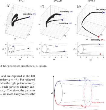
3.2 The second scenario
We consider now particles starting from the boundaryz= −λ. In this case the particles approach the neutral plane with-out crossing the uncertainty curve due to the shrinking of the uncertainty curve fors6=0 (see scheme in Fig. 5). Such par-ticles do not accomplish a half-turn aroundBz, but oscillate
around field lines. An example of such a trajectory is shown in Fig. 4d. This type of motion resembles the classical gy-rocentre motion without the demagnetization in the neutral plane. Therefore, particles starting atz= −λcannot be re-flected from the CS and transit through it. This scenario is realized for realistic position of boundaries (λ≥1) and not very smallBy(s > (π−1ln 2)κ).
3.3 The third scenario
This scenario concerns particles trapped within the CS. For these particles the coordinates of mirror points κxm are
smaller than the corresponding coordinate of the boundary
κx¯. There are two possible subscenarios of motion for such particles.
Due to geometrical jumps ofIz the particles can change
Izvalue at the uncertainty curve, and thus change the
corre-sponding mirror pointsκxm. However, for each trajectory the
number of such jumps with changing the value ofIzis finite,
Fig. 5. Schematic view of particle trajectory.
i.e. the number of possible values ofIzis finite. This number
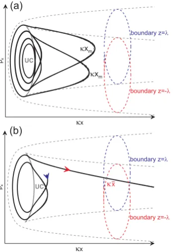
depends only on thesparameter (see Artemyev et al., 2013). Therefore, there are particles with all possible values ofκxm
smaller thanκx¯ (see the scheme in Fig. 6a). These particles cannot escape from the CS, and only quasi-random dynami-cal jumps ofIz may change this situation (see the next
sec-tion). An example of such a trajectory is shown in Fig. 7a. In the absence of dynamical jumps ofIz, these particles would
have been trapped inside the CS forever.
The second subscenario corresponds to particles withIz
decreasing due to geometrical jumps so substantially that the new mirror points appear at κxm> κx¯ (see the scheme in
Fig. 6b). These particles can make a half-turn aroundBzand
Fig. 6. Schematic view of particles’ trajectories.
Fig. 7. Particles’ trajectories and corresponding projections onto the (κx, px)plane.
4 Destruction of the quasi-adiabatic invariant
The quasi-adiabatic invariantIzis an approximate invariant
of motion. Far from the separatrix,Izis conserved with the
accuracy∼κ (see Arnold et al., 2006). One can introduce the improved quasi-adiabatic invariant J=Iz+κu where
u(z, pz, κx, px), is defined at each point of the phase space
Fig. 8. Trajectories of two particles in the system withκ=0.01.
(z, pz, κx, px)for fixed energyH=1/2 (ucannot be
deter-mined only at the separatrix). Far from the separatrix,J is conserved with the accuracy∼κ2. Functionuis defined in Appendix A2.
As a result of separatrix crossings, the invariantJ expe-riences a jump1J=1Jgeom+1Jdyn, where the geomet-rical jump 1Jgeom is defined by the system geometry, and the dynamical jump 1Jdyn∼κlnκ depends on a variable
ξ∈(0,1), which characterizes the precise position of a sepa-ratrix crossing in the plane(z, pz), and can be considered as a
quasi-random variable (see Appendix A). Thus, values of dy-namical jumps can be treated as random. Dydy-namical jumps result in destruction of the quasi-adiabatic invariant, i.e. par-ticles slightly change their trajectories in the plane(κx, px)
at every crossing of the uncertainty curve. Examples of par-ticle trajectories calculated on a long-time interval are shown in Fig. 8 for two values ofs. One can see that both particle trajectories acquire the spread over the plane(κx, px). For a
sufficiently long time interval the particle trajectory should fill a substantial part of the plane(κx, px)(the area of this
covered part does not depend onκ) .
To demonstrate the effect of1Jdynwe calculate the par-ticle trajectory on a long time period and show distributions ofIzvalues measured at the moment of particle crossing of
the neutral planez=0 withpx=0 (see Fig. 9). For the
sys-tems withs6=0 and a very small value ofκ we have sev-eral values ofIz. This is the effect of trajectory splitting due
Fig. 9. Distributions ofIzat various values ofsandκ. Each
distri-bution contains 103values.
(but having a finite width) distributions around these max-ima. This is the effect of Iz destruction due to dynamical
jumps. For the system withs=0 we observe the same result, but with the single peak value ofIz. An increase ofκresults
in the increase of the width ofIzdistribution due to
intensi-fication of the destruction ofIzbecause of dynamical jumps.
The spreading of theIzdistribution around the initial value
(this value corresponds to the maximum of the distribution at
s=0) is similar for systems withs=0 ands6=0. However, due to splitting of trajectories caused by geometrical jumps (the appearance of several maxima in theIz distribution for
systems withs6=0), the whole range of accessible values of
Izis wider for systems withs6=0. In the case ofκ=0.1,
dy-namical jumps become comparable with geometrical jumps. As a result, there is a strong stochastization of particle mo-tion.
5 Statistical aspects of particle motion
In this section we describe the probabilistic nature of parti-cle captures in the potential wells at the uncertainty curve. When particles leave the neutral plane and cross the uncer-tainty curve, they can enter one of the two small potential wells. Capture in the left well corresponds to motion towards the bottom boundaryz= −λ, while capture in the right well corresponds to motion towards the top boundaryz=λ. For each trajectory this choice is determined by the coordinates of the separatrix crossing in the plane(z, pz). Because
vari-ables(z, pz)evolve fast and periodically, even a small
vari-ation of initial coordinates can result in a different choice of the potential well. Thus, the choice of the left or right potential wells can be considered as a probabilistic process
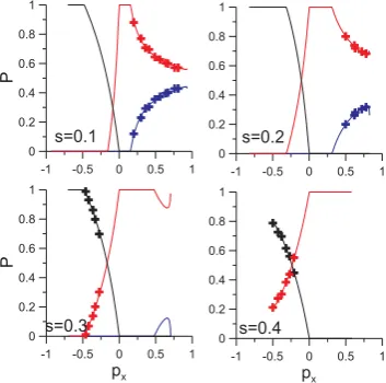
Fig. 10. Analytical profiles of probabilities as functions ofpxalong
the uncertainty curve. Crosses show numerical results. Black colour is used forP, red forPl, and blue forPr.
with certain probabilitiesPl≥0,Pr≥0. When particles
ap-proach the uncertainty curve being within one of the two possible potential wells, there is also a certain probability of capture in the single wellP =1−Pr−Pl. Analytical
expres-sions for these probabilities were derived in Artemyev et al. (2013). ProbabilitiesPl,r,Pdepend on coordinates of the un-certainty curve crossing in the plane(κx, px). Probabilities
Pl,r are positive if areas surrounded by corresponding sepa-ratrix loops (see Fig. 1) are growing. If areas decrease, then the corresponding probabilities are equal to zero.
Fors=0 we have the symmetric system withPl=Pr=
0.5 forpx>0 andP =1 forpx<0. For four values ofs >0
we plotPr,landP as functions ofpx along the uncertainty
curve (see Fig. 10). With the increase ofsthe probabilityPr
decreases, and fors >0.35 we havePr=0. Thus, for s >
0.35, particles cannot be captured in the right potential well at the uncertainty curve. Also fors6=0 we havePl>0 for px<0. Thus, when particles approach the uncertainty curve
while inside the right small well, they can be captured either in the single well or in the small left well.
To check the analytical expressions for the probabilities, we use two simulations with ensembles of particles. In the first simulation we takes=0.1 ands=0.2. We run 104 par-ticles with the same quasi-adiabatic invariant, the same en-ergy, and the uniform distribution of initial coordinates along the trajectory in the plane (z, pz), i.e. a number of
parti-cles in a small trajectory fragment centred at a certain value of pz is inverse proportional to pz value. All the particles
are initially located inside the single potential well (px=0,
crosses in Fig. 10 fors=0.3,s=0.4). One can see that nu-merical results agree with analytical expressions quite well.
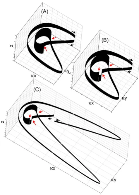
To illustrate the probabilistic nature of a choice of potential wells (where particles are captured), we present three real-izations of one particle trajectory. All these realreal-izations start from the same point in the plane(κx, px)(see Fig. 11). The
black arrows show the start and finish points of trajectories. Red arrows indicate points where the particle changes the potential wells. Corresponding projections of particle trajec-tories in the plane(κx, px)are shown in Fig. 12.
Let us describe the trajectories in Figs. 11 and 12. First, the particle starts moving inside the right potential well. Then the particle approaches the uncertainty curve atpx≈ −0.4.
At this point the particle should leave the right well, because the corresponding area decreases (see detailed description of area and probability distributions along the uncertainty curve in Artemyev et al., 2013). Areas of the left well and the single well are increasing, and thus there are certain possibilities to be captured in the single well with the probabilityP and in the left well with the probabilityPl,1. In the first case the
particle accomplishes a half-turn aroundBzand approaches
the uncertainty curve while within the single well withpx≈
0.4. At this point the particle can be captured only in the left well (as the area of the right well decreases). This is the realization (A) in Fig. 11.
In the second case the particle is reflected from the un-certainty curve inside the left well withpx≈ −0.4, and
ap-proaches this curve again withpx≈ −0.6. At this point the
areas of both small potential wells decrease and the parti-cle can be captured only in the single well. Then the partiparti-cle makes a half-turn aroundBzand approaches the uncertainty
curve inside the single potential well withpx≈0.6. At this
point the areas of both small potential wells increase and the particle can be captured in the right well with the probability
Pr,2and in the left well with the probabilityPl,2. In the first
case we have the realization (B), and the second case corre-sponds to the realization (C) in Fig. 11. Such splittings of the single trajectory into three realizations are possible only for the non-symmetric system withs6=0 when the two areas of small potential wells evolve asynchronously.
Fig. 11. Three realizations of particle trajectories starting from one point in the plane(κx, px).
6 Discussion
Trapped and transient particles play different roles in the CS. Trapped particles with reflection points below the CS bound-aries|z| =λ accomplish their oscillation motion inside the CS (their adiabatic trajectories withIz=const are closed in
the(κx, px)plane). As a result, the total electric current
Fig. 12. Three panels show projections of trajectories from Fig.11 to the plane(κx, px). Probabilities of all trajectories corresponds to
combination of probabilities at the uncertainty curve.
particle detrapping, the CS lifetime is limited by the time of total stochastization of particle motion (Zelenyi et al., 2002a, 2003). We obtain an important result for dynami-cal jumps in the CS with By6=0: in contrast to the
sym-metric system, whereh1Jdyni =0, in asymmetric systems we have h1Jdyni 6=0 (see Appendix A). This effect dras-tically changes the characteristic time of stochastization of particle motion.Izof each particle changes by a value ∼κ
(here for simplicity we omit lnκ) in the course of one cross-ing of the uncertainty curve (one crosscross-ing of the separatrix). During one period of motion in the(κx, px)plane (the
pe-riod is∼κ−1) particles are crossing the uncertainty curve twice. Ifh1Jdyni =0 (s=0 case), then the averaged jump is equal to zero, buth(1Jdyn)2i ∼κ2is finite. Thus, we need time∼κ−3to change the invariant value substantially (the situation is different in the special case of when an initial value ofIzis comparable withκ; see Vainshtein et al., 1999;
Vainchtein et al., 2005). In the case of non-zero average value
h1Jdyni 6=0 (s6=0 case) there is a drift in the space of the invariants. This drift results in effective evolution ofIz, and
as a result, the time required for the substantial change ofIz
is aboutκ−2. For parameters of the Earth’s magnetotail this effect results in the decrease of the stochastization time for one order of magnitude. Previous estimates gave the time of the CS destruction due to stochastization around tens of min-utes forκ≤0.1 (Zelenyi et al., 2002a, 2003). In the case of finiteBy (for By≥Bz) the time of stochastization of
parti-cle motion (and corresponding CS destruction) becomes of the order of a few minutes. This is a rather small time in-terval for the Earth’s magnetotail. Thus, the existence of the CS with small but finiteBy ((π−1ln 2)κ < s <0.35) seems
to be impossible without a certain mechanism of particle de-trapping. The role of this mechanism can be played by the earthward convection, when trapped particles get a chance to escape from the CS region due to the earthward drift motion. In addition, any (even weak) gradient ofBzalong thexaxis
results in the drift of trapped particles in they direction. In this case trapped particles can already contribute to the total
cross-tail current, and thus help support the CS configuration (see discussion in Artemyev and Zelenyi, 2013).
Increase of the stochastization rate of particle motion with the increase ofBy(untils <0.35) is also important due to the
additional role played by the trapped population. The trans-verse electric field exists in the Earth’s magnetotail (see Kan, 1990; Angelopoulos et al., 1993) and in reconnected CSs of the solar corona (e.g. Litvinenko, 1996). Thus, stochastic motion of trapped particles can contribute to the transverse collisionless conductivity in the CS (Horton and Tajima, 1990). The magnitude of such conductivity strongly depends on the level of stochasticity of particle motion (Holland and Chen, 1992; Greco et al., 2000; Numata and Yoshida, 2002). Thus, enhancement of stochastization should result in an in-crease of collisionless conductivity and support the develop-ment of various resistive instabilities in the CS (see review by Horton, 1997, and references therein).
Although we obtain non-zeroh1Jdyni(averaging overξ; see Appendix A), we should also take into account the con-servation of phase volume in the system. This requirement can be written as a kinetic equation df/dt=0 for the dis-tribution function of particles f, where d/dt is the total derivative (Pitaevskii and Lifshitz, 1981). Absence of par-ticle collisions results in the conservation of the phase vol-ume, and forbids directed drifts of particles in the invari-ant space (Sinitsyn et al., 2011), i.e. the double averaged
hh1JdyniiI
z (the second averaging is performed over
adia-batic invariants) should be equal to zero. Therefore, we ob-tain that for eachIzan averaged valueh1Jdyniis non-zero,
but for all population of particles we have only redistribution of invariants without the appearance of any particle fluxes in the phase space. However, we should mention that the presence of the boundaries z= ±λ can result in non-zero-averaged jumpshh1JdyniiI
z6=0 with corresponding particle
drift in the phase space (Zelenyi et al., 2003).
The effect of asymmetry of particle reflection/transition in the CS withBy6=0 has been mentioned by many authors
with decrease of the distance between the neutral plane and positions of corresponding reflection points. A decrease in the length of the uncertainty curve with the increase ofBy
results in the absence of the uncertainty curve crossings for particles from the Southern Hemisphere (from the boundary
z= −λ). These particles cannot be reflected from the CS and even cannot be scattered in the CS. Their trajectories cross the neutral plane without a half-rotation around Bz. Thus,
such particles come directly to the boundaryz=λ(normally gyrating around field lines). Roughly speaking, in systems withBy6=0, the probability of particle reflection from the
CS to the initial hemisphere decreases with the increase of
By. For large enoughBy> B0
√
L/ρ0, the scattering of
par-ticles is absent (see Artemyev et al., 2013). Thus, all parti-cles cross the neutral plane moving along trajectories, which can be described by the guiding-centre theory. This effect of asymmetry of the CS interaction with particles can play an important role in the Earth’s magnetotail, where By is
provided by penetration of the interplanetary magnetic field (Cowley, 1981; Wing et al., 1995), by deformation of the neutral plane (Petrukovich, 2009) or by local currents (Arte-myev, 2011; Rong et al., 2012). Particles usually come to the CS of the Earth’s magnetotail from the sources in the South-ern and NorthSouth-ern Hemisphere. If these sources have different intensities, butBy=0, then symmetric reflection/transition
results in symmetric field-aligned flows of particles in both hemispheres. However, even smallBy6=0 results in
asym-metric reflection and asymasym-metric flows of ions from the mag-netotail towards the ionosphere. Auroral phenomena in the ionosphere are often considered as projections of particle flows from the magnetotail (see, e.g. Østgaard and Laundal, 2012, and references therein). Thus, the asymmetry of au-roral phenomena in the case ofBy6=0 (Liou and Newell,
2010; Lukianova et al., 2012) can be partially explained by asymmetry of CS interaction with ions and corresponding asymmetry of compensation of electron currents.
One of the most beautiful manifestations of the nonlinear particle dynamics in the CS is the so-called resonant interac-tion: particles with a certain value of energy (i.e. the certain value ofκ) are not scattered in the CS (Chen and Palmadesso, 1986; Burkhart and Chen, 1991; Büchner, 1991). This res-onant effect is responsible for the formation of beamlets – coherent beams of accelerated particles (Ashour-Abdalla et al., 1992; Grigorenko et al., 2005, 2011). Resonant inter-action can be explained by a compensation of two successive
shown that fors > (π−1ln 2)κand fixedκ, the simultaneous compensation of two successive dynamical jumps is possi-ble only for relatively small group of particles with a certain value of the quasi-adiabatic invariant. The population of res-onant particles for fixedκ decreases with the increase ofs. As a result, the effect of resonant interaction with the CS can-not be seen for a large population of particles in systems with
s > (π−1ln 2)κ.
7 Conclusions
In this paper we have described effects of the magnetic field shear on non-adiabatic behaviour of charged particles. The main conclusions are listed below:
1. The presence ofBy6=0 results in asymmetry of
par-ticle reflection from (and transition through) the CS. ForBy>0, particles from the Southern Hemisphere
(z >0) are more likely to cross the CS. The probability of the CS crossing for these particle increases with the growth ofByand forBy>0.35B0
√
L/ρ0all particles
from the Southern Hemisphere are crossing the CS. Particles from the Northern Hemisphere are crossing the CS without scattering already fors > (π−1ln 2)κ
(i.e.By> (π−1ln 2)Bz). These particles cannot be
re-flected from the CS in the case ofBy>0. The situation
is mirror symmetric forBy<0 (Southern Hemisphere ←→Northern Hemisphere).
2. In systems with By6=0 the intensification of
parti-cle scattering (and corresponding chaotization of mo-tion) occurs. Average values of dynamical jumps of the quasi-adiabatic invariant are not equal to zero. The presence of geometrical jumps due to the emerging ef-fective asymmetry of the system withBy6=0 helps to
destroy the adiabaticity.
3. Finite By> (π−1ln 2)Bz destroys the resonances in
the CS. In systems with large enoughBythe resonant
(2013):
Sl,r= −As±2π zc(g2c+z2c)
As= −4zc(gc2+zc2)arctan
zc
gc
−4z2cgc−83g3c
2l,r=2Azc(2A2±π s)
A2=sarctan
zc
gc
−zc
sgc,
wheregc=g(zc)and
g(z)=
q
Azc−s2−
1 4(z+zc)
2, A
zc=
1+zc2
s
−1/2
We also introduce the asymptotic expression for the period of particle fast oscillations Tl,r=bl,r−aln|E|, where E=
H−hc and hc is the energy at the saddle point zc of the
separatrix (see Fig. A4):
hc=
1
2(px−szc)
2+1
2
κx−1
2z
2
c
2
.
Coefficientsbl,randaare derived in Sect. A1.
To evaluate jumps of the quasi-adiabatic invariant we have to introduce the improved invariantJ=Iz+κu, where the
expression foruis derived in Sect. A2. Finally, we use the relation between the valueJ−of the improved invariant be-fore crossing of the uncertainty curve and its valueJ+after crossing. This relation can take several forms corresponding to different transitions. Here we write the general expression for relation betweenJ− andJ+ (see Neishtadt, 1987) and then reduce it to the form corresponding to the Hamiltonian system (1).
For the transition from the single well to one of two small wells, when areas of both small wells grow, we have 2π J−=(Sl+Sr)+κu,J+=Jl,r. Here areasSl,rare defined
at points where adiabatic trajectories (corresponding to the initial value of the invariantIzfar from the uncertainty curve)
cross the uncertainty curve. The relation betweenJ−andJ+
can be written as (Neishtadt, 1987)
2π Jl,r=Sl,r+2π θl,rκu˜+κ dl,r−θl,r(dr+dl)
+κa2l,r
ξ−1
2
ln(κ2l,r)−2θl,rln(κ2)
+κa2l,rln 0(ξ )0 θl,r(1−ξ )0(1−θl,rξ )/(2π )3/2
−κ2l,rξ−1
2
bl,r−θl,r(br+bl)
−κθl,rξ−1
2
Sl,r, S +O(κ3/2lnκ),
(A1)
describes the transitions from the left small well to the single well (with the same relations 2π J−=(Sl+Sr)+κu,J+=
Jl,r) when the area of the right well increases. In this case we have2r>0,2l<0,2 <0 andξ∈(0,1− |2l/2r|).
Here we should mention that Eq. (A1) also contains a term
O(κ3/2(1−ξ )−1)(see Neishtadt, 1987). Below, we omit this term and assume thatξ is far from 1 (i.e. 1−ξκ).
For the transition between small wells (when2r<0 and 2l>0) we have (see Neishtadt, 1987)
2π Jl=Sl+2πθ˜−1κu˜r+κ
dl− ˜θ dr
+κa (1−ξ ) (2rln(κ2l)−2lln|κ2r|)
−κa2l
ln
2π(1−ξ )
q
| ˜θ|
−ln0(ξ )0(1+ ˜θ− ˜θ ξ )
+κ (1−ξ ) (2lbr−2rbl)
−κ (1−ξ ){Sl, Sr} +O(κ3/2lnκ),
(A2) wheredl,r=ul,r/2π=0 (see Sect. A2),u˜r=Jr−Sr/2π6=0
andθ˜=2r/2l<0. Hereξ ∈(0,1)for2 >0 andξ∈(1−
|2l/2r|,1)for2 <0.
Terms{Sl,r, S} = {Sl, Sr}and{Sl, Sr}in Eqs. (A1) and (A2) are defined in Sect. A3. In Sect. A1 we show thatblis equal tobr (we introduce b=bl,r). Then we have bl,r−θl,r(bl+
br)=b(1−2θl,r). Finally, for the transition between the sin-gle well and small wells we have
1J =Jl,r+−J−=1Jl,rgeom+1Jl,rdyn+O(κ3/2lnκ) 1Jl,rgeom= 1
2π(Sl,r−S)= −
1 2πSr,l
1Jl,rdyn=κa2l,r
ξ−1
2
ln(κ2l,r)−2θl,rln(κ2)
−κa2l,rln
(2π )3/2
0(ξ )0 θl,r(1−ξ )0(1−θl,rξ )
−κ2l,rb
ξ−1
2
1−2θl,r+κθl,ru˜
−κθl,r
ξ−1
2
{Sl,r, S}, (A3)
−κ(1−ξ ){Sl, Sr}. (A4)
Here we define the geometrical jump in Eqs. (A3) and (A4) as the difference of unperturbed areas surrounded by the separatrix loops before and after the separatrix crossing.
For the system with the symmetric phase portrait (s=0) we haveSl=Sr=S/2,2l=2r=2/2. Then the transition between two small wells is impossible. For the transition be-tween the single well and one small well we have
1Jl,rgeom= −1
4πS= −
1 2J
−
1Jl,rdyn= − 1
2πκa2
ξ−1
2
ln 2
− 1
2πκa2l,rln
(2π )3/2 0(ξ )012(1−ξ )0(1−1
2ξ )
= − 1
2πaκ2l,r
ξ−1
2
ln 2
− 1
2πκa2l,rln(2 3
2−ξsinπ ξ )
= − 1
2πκa2l,rln(2 sinπ ξ ),
where we use Euler’s reflection formula and Legendre’s du-plication formula for gamma functions (see Gradshteyn and Ryzhik, 2007):
0(ξ )012−1
2ξ
0(1−1
2ξ )
=0(ξ )012−1
2ξ
0(12−1
2ξ+ 1 2)
=21−2(12− 1 2ξ )
√
π 0(ξ )0(1−ξ )=2ξπ3/2/sinπ ξ.
Thus, for the symmetric system (s=0), the geometri-cal jump 1Jl,rgeom is equal to half of J in the single po-tential well. As a result, we can renormalize J to cancel
1Jl,rgeom: we defineJ as a half-value of the corresponding variable (i.e. J→J /2) when particles oscillate in the sin-gle well. Section A1 givesa=1/gc, while2l,r=4AzcA2=
4(Azczc/s)gc= −4pxgc. Thus, fors=0 we obtain the
well-known expression for the dynamical jump (Timofeev, 1978; Neishtadt, 1986; Cary et al., 1986; Neishtadt, 1987; Büchner and Zelenyi, 1989),
1Jdyn= −2
πκpxln(2 sinπ ξ ).
Fig. A1. Geometrical jumps for systems with variouss.
For asymmetric systems (s6=0) we plot1Jgeomas func-tions of the coordinate px along the uncertainty curve
(Fig. A1). One can note that the differenceSl−Sris linearly
proportional topx. This dependence can be easily obtained
analytically as well.
For the symmetric systems=0 the average value of the dynamical jump is equal to zero:
D
1Jdyn
E
ξ
= −2
πκpx 1
Z
0
ln(2 sinπ ξ )dξ=0.
D
1JdynE ξ
=κa2l,rG1(θl,r), 2l,r>0
D
1Jdyn
E
ξ
=κa2lG2(θ )˜ +
1
2κ{Sl, Sr}, 2l>0, 2r<0, 2 >0
D
1Jdyn
E
ξ
=κa2lG3(θ )˜ +
1 2 ˜
θ−2κ{Sl, Sr}, 2l>0, 2r<0, 2 <0 ,
and for the transition between small wells
1Jdynξ=1
2κa (2rln|κ2l| −2lln|κ2r|)
+1
2κb (2l−2r)
−κa2lG4(θ )˜ −12κ{Sl, Sr}, 2l>0, 2r<0, 2 >0
1Jdyn
ξ=
1
2κa (2rln|κ2l| −2lln|κ2r|)
+1
2κb (2l−2r)−κa2lG5(θ )˜
−1
2θ˜
−1κ{S
l, Sr}, 2l>0, 2r<0, 2 <0,
where
G1(θl,r)=
1
R
0
ln (2π )3/2dξ
0(ξ )0(θl,r(1−ξ ))0(1−θl,rξ )
G2(θ )˜ = 1
1+ ˜θ
1+ ˜θ
R
0
ln (2π )3/2dξ
0(ξ )0
1 1+ ˜θ(1−ξ )
0(1− 1
1+ ˜θξ )
,θ >˜ −1
G3(θ )˜ = −1
1+ ˜θ
1
R
2+ ˜θ
ln (2π )3/2dξ
0(ξ )0
1 1+ ˜θ(ξ−1)
0(1− 1
1+ ˜θξ )
,θ <˜ −1
G4(θ )˜ = 1
R
0
ln 2π(1−ξ )
√
| ˜θ|
0(ξ )0(1+ ˜θ− ˜θ ξ )dξ , ˜
θ >−1
G5(θ )˜ =−θ˜1
1
R
(θ˜+1)/θ˜
ln 2π(1−ξ )
√
| ˜θ|
0(ξ )0(1+ ˜θ− ˜θ ξ )dξ , ˜
θ <−1.
Profiles of functionsGiare shown in Fig. A2
For several values ofswe plot average dynamical jumps
h1Jdyniξ as functions of the coordinate of uncertainty curve crossingpxin Fig. A3. Here we ploth1Jdyniξwithout terms ∼ {Sl, Sr}(analytical expressions for{Sl, Sr}can be found in Sect. A3).
A1 Period of fast oscillations
In this subsection we derive the asymptotic expression for the period of fast oscillationsTl,r=bl,r−aln|E|in the left and
Fig. A3. Dynamical jumps in the system with variouss without terms∼ {Sl, Sr}.
right potential wells. From the general theory it is well known that Tl=Tr for Hamiltonian systems like (1) (see Arnold,
1988). Thus,bl=br, and we can derive the expression only
forTr:
Tr=2 z+ Z
z∗
dz
r
2H−(px−sz)2−
κx−1
2z2
2
,
wherez+is shown in Fig. A4 andz∗corresponds to the
left-most point of the trajectory inside the right separatrix loop. The difference between thez∗value and thezc value is
de-termined by the particle energy. We introduceza> z∗> zc
and divide the integralTr into two parts (1z=za−zc>0
is small enough). The first part of the integral corresponds to integration along the small fragment of the particle tra-jectory inside the separatrix loop in a close vicinity toz∗. To perform this integration correctly, Tr should be
rewrit-ten asTr=
R
dpz/p˙z. However, for Hamiltonian (1) it is well
known that integration overpz inside the separatrix loop in
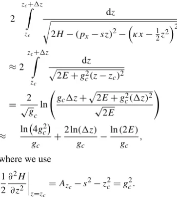
zc
2E gc(z zc)
=√2
gcln
gc1z+
p
2E+g2
c(1z)2 √
2E
!
≈ ln 4g
2
c
gc
+2 ln(1z)
gc
−ln(2E)
gc
,
where we use 1
2
∂2H ∂z2
z=zc
=Azc−s
2−z2
c=gc2.
The second part can be considered as the integral along the separatrix, because we integrate over |z−zc|> 1z. In
this case we have (see Artemyev et al., 2013) 2H−(px−sz)2−(κx−12z2)2
=(z−zc)
Azc−s
2−1 4(z+zc)
2
and
2
z+ Z
zc+1z
dz (z−zc)
q
Azc−s2−
1
4(z+zc) 2
≈ 2
gc
ln
(z+−zc)
1z
4gc2
2(g2
c+z2c)−zc(z++zc)
= −2 ln(1z)
gc
+2 ln 4g
2
c
gc
−ln g
2
c+z2c
gc
,
where we take into account thatz±= ±2
p
g2
c+z2c−zc. The
final expression for the period is
Tl,r= −
ln(2E) gc
+3 ln 4g
2
c
gc
−ln g
2
c+z2c
gc
.
Therefore, we have
a=1/gc
bl=br=6 ln(2gc)
gc
−ln g
2
c+z2c
gc
−ln(2)
gc
.
A2 The improved quasi-adiabatic invariant
In this section we derive the asymptotic expression for the improved quasi-adiabatic invariantJ=Iz+κufor pz=0,
whereuis defined as (see Neishtadt, 1987)
R
(T /2−t ){E, hc}dt.
u= 1 4π T Z 0 ∂E ∂px t Z 0 ∂E ∂κxdt
0
dt−
T Z 0 ∂E ∂κx t Z 0 ∂E ∂px
dt0
dt + 1 2π T Z 0 T
2 −t
∂hc ∂px ∂E ∂κx− ∂hc ∂κx ∂E ∂px dt .
HereT (κx, px)is the period of fast motion. Integration is
performed along a trajectory with a certain initial point in the plane(z, pz). We choose this point aspz=0, and as a result,
the lower limit of integrationt=0 corresponds to the starting point where the trajectory crosses thepz axis (the leftmost
point of the trajectory). We consider one of the two potential wells (the right one). The last term ofucan be written as
1 2π T Z 0 1 2T−t
{E, hc}dt ,
where{. . .} is the Poisson bracket. We divide this integral into two parts:t∈ [0, T /2]andt∈ [T /2, T]. The expression
{E, hc}does not depend onpz, and thus it has the same
val-ues fort andt+T /2. ExpressionT /2−t= −(t−T /2)is positive fort∈ [0, T /2]and negative fort∈ [T /2, T]. As a result, the total integral is equal to zero (see the scheme in Fig. A4).
Now we consider the first two integrals in the expression forufor the right well. The inner integrals are
t
R
0
∂E ∂κxdt
0= −1 2
(
={zc,z}
6 , t <
1 2T
={zc,z+}
6 + =
{z,z+}
6
= −1
2=
{zc,z+}
6 ±
1 2=
{z,z+}
6
t
R
0
∂E ∂pxdt
0= −s
(
={zc,z}
0 , t < 1 2T
={zc,z+}
0 + =
{z,z+}
0
= −s={zc,z+}
0 ±s=
{z,z+}
0 ,
where±corresponds tot < T /2 and t > T /2, and we use
pz2=2(H−hc)=(z−zc)2g2(z)(see Artemyev et al., 2013).
The first integral in expression foruis T R 0 ∂E ∂px t R 0 ∂E ∂κxdt
0
! dt
=4sgc=
{zc,z+}
0 =8sgc
π
2−arctan
zc
gc
,
and the second integral is
T R 0 ∂E ∂κx t R 0 ∂E ∂pxdt
0
!
dt=s={zc,z+} 6
π−2 arctanzc
gc
=
=4sπgc−8sgcarctan
zc
gc
.
Then, the difference of the first and the second terms is equal to zero, andu=0 for the right potential well (at
pz=0). The same conclusion is valid for the left well and
for the single well. Moreover, one can show thathuiξ=0 (see details in Neishtadt, 1987).
A3 Calculation of{Sl,r, S}
Here we derive the expression for{Sl,r, S}. Due toS=Sl+Sr
we need to obtain the expression{Sl, Sr}, where
Sl,r=2
zmax l,r
Z
zminl,r
p
2U (κx, px, zc)−2U (κx, px, z)dz
andzminl,r =z−, zc,zmaxl,r =zc, z+, 2U=2H−p2z (see
Arte-myev et al., 2013). We can write 2U (κx, px, zc)−2U (κx, px, z)=
(px−szc)2+(κx−12zc2)2−(px−sz)2−(κx−12z2)2
= −2spx(zc−z)−κx(z2c−z2)+s2(z2c−z2)+14(z 4
c−z4).
px=(zc/s)(s2−Azc)withAzc=(1+z
2
c/s2)−1/2(see
Arte-myev et al., 2013). The corresponding integrals are
zmaxl,r
R
zl,rmin
z2c−z2
√
2U (zc)−2U (z)dz
=4gc zmaxl,r
R
zl,rmin
zc−z
√
2U (zc)−2U (z)dz
=π±2 arctanzc
gc
.
Derivatives∂Sl,r/∂zc∼∂U (zc)/∂zcare equal to zero due
to the definition ofzc. Thus, finally we have
∂Sl ∂κx ∂Sr ∂px −∂Sl ∂px ∂Sr
∂κx =32sgcarctan
z c gc . Appendix B Resonances
In this appendix we describe the effect of resonant interac-tion of a particle with the CS. In the course of interacinterac-tion with the CS, particles cross the uncertainty curve (and the separatrix) twice: when particles approach the neutral plane moving along the field lines, and when they leave the neutral plane after a half-turn aroundBz. Therefore, there are two
dynamical jumps of the quasi-adiabatic invariant.
For the symmetric system (s=0) we have the expression for the dynamical jump 1Jdyn= −(2/π )κpxln(2 sinξ π ),
whereξ∈(0,1)is a random value (see Appendix A). Thus, the sum of two successive jumps is
X
1Jdyn= −2
πκpxln
2 sin
π ξ
2 sinπ(ξ+1ξ )
,
where1ξ is a difference of phases between two separatrix crossings. The full expression for1ξ can be found in Neish-tadt and Vasiliev (2005):1ξ+ξ =Frac(W−ξ ), where
W= 1
κπ
κx∗
Z
κx˜
z
px
dκx
Fig. B1. Schematical view of a particle trajectory with two crossings of the uncertainty curve.
Frac(·)denotes the fractional part of a number in brackets
(·),κx∗is the coordinate of uncertainty curve crossings and
z(κx)is the frequency of fast oscillations:
z=2π
I dz/pz
−1
.
If1ξis equal toπ−2ξ(i.e.W=π), we haveP1Jdyn=
0. This condition corresponds to the equationW=π, which is independent ofξ. Thus, the conditionP
1Jdyn=0 can be simultaneously satisfied for a large particle population. The equationW=π can be solved with regard toκ, and corre-sponding solutions are called resonantκvalues (Büchner and Zelenyi, 1989; Zelenyi et al., 2013).
To investigate the same effect of the resonance for systems withs6=0, we write equations of the uncertainty curve in the
(κx, px)plane (see Artemyev et al., 2013)
Fig. B2. Fragments of three trajectories and corresponding depen-dence ofπ/ zonpx.
px=(zc/s)(s2−Azc)
κx=1
2z 2
c+Azc
.
One can see that the sign ofpxis defined by the sign ofzc
(becauseAzc−s
2>0 for entire range ofz
c). Due to the
sym-metry of the phase portrait of the system in the plane(κx, px)
relative topx=0, particles that crossed the uncertainty curve
at px= −px∗<0 should cross it again at px=p∗x>0. A
schematic view of such a trajectory is presented in Fig. B1. We consider the particles that come to the uncertainty curve inside the right well and after the second crossing are cap-tured in the left well. These particles can return to the initial coordinateκxin the opposite side relative to the neutral plane
z=0. For these particles the coordinate of the saddle point in the second crossing z(c2) is equal to−z(
1)
c , wherez(
1)
c is
the coordinate of the saddle point in the first crossing. Be-causeSr(zc)=Sl(−zc)(see expression forSl,rin Appendix
A), we haveSr(1)=Sl(2). Thus, two successive geometrical
jumps compensate each other for such trajectories.
The ratesκ2l,rof evolution of areas can be presented as a
sum2l,r=4AzA2±2π sAzc. Thus, we haveθ=θ
(1)
r =θl(2).
Fig. B3.W as a function of Iz for various s (to substitute
val-ues ofW in the equation for dynamical jumps, one should take Frac(W/κ)).
1J(dyn1,2)= ±κ2
(1)
r 2π
ξ(1,2)−1
2
aln κ2(r1)
(κ2)2θ−b (1−2θ )
∓κa2
(1)
r 2π ln
(2π )3/2
0(ξ(1,2))0(θ (1−ξ(1,2)))0(1−θ ξ(1,2)),
where a=a(zc)=a(−zc) and b=b(zc)=b(−zc) (see
Sect. A1). The sum of these jumps gives P
1Jdyn=κ2
(1)
r 2π 1ξ
aln κ2
(1)
r
(κ2)2θ−b (1−2θ )
−κa2
(1)
r 2π ln
0(ξ(2))0 θ (1−ξ(2))
0(1−θ ξ(2)) 0(ξ(1))0(θ (1−ξ(1)))0(1−θ ξ(1)),
where 1ξ=ξ(2)−ξ(1). One can see that the condition
1ξ=const−2ξ(1) does not obviously result inP
1Jdyn=
0. Thus, the resonant conditionP
1Jdyn=0 corresponds to a certain equation, which depends onξ(1)and on coordinates of the uncertainty curve crossing. Such a condition cannot be satisfied simultaneously for a large particle population. This is the first effect, which results in the destruction of reso-nances.
Let us consider the second effect, which is responsible for destruction of resonances. This effect corresponds to depen-dence of the frequencyz on the quasi-adiabatic invariant
Iz:
Fig. B2. At the vicinity of the uncertainty curve the frequency
ztends to zero. This is an effect of the logarithmic
singu-larity of the frequency of particle oscillations near the sepa-ratrix.
We calculateW for Iz≥Iz(0), where Iz(0) corresponds to
the trajectory crossing the uncertainty curve at the endpoints (see Fig. B2). Corresponding dependencies ofW onIz are
shown in Fig. B3. One can see that for smalls the function
W (Iz)tends to 0.76/κ asIz(0)→0 (this value can be
calcu-lated analytically; see Büchner and Zelenyi, 1989).
For smallsthe derivative∂W/∂Izis small enough. Thus,
if a value ofκin the system is suitable to obtain the resonant value of1ξ forIz=Iz(0), then for particles with otherIz, the
corresponding 1ξ should have similar values. As a result, the resonant condition (condition forκ) is satisfied for parti-cles with variousIz(see discussion in Büchner and Zelenyi,
1989).
Increasing s results in the increase of the derivative
∂W/∂Iz. Thus, 1ξ changes more substantially withIz for
s >0. It means that even if κ has a suitable (resonant) value to obtain the resonant value of 1ξ for Iz=Iz(0), for
particles with other values of Iz, the corresponding1ξ ∼
(∂W/∂Iz)(Iz−Iz(0))should be far from the resonant value.
This results in a decrease in the number of particles for which the resonant condition is satisfied for the sameκ.
Acknowledgements. We are very grateful to A. A. Vasiliev for
useful discussion. This work was supported in part by the RF Presidential Program for the State Support of Leading Scientific Schools (project NSh-2519.2012.1) and the Russian Foundation for Basic Research (projects 11-02-01166, 13-01-00251).
Edited by: J. Büchner
Reviewed by: H. Karimabadi and A. Anastasiadis
Arnold, V. I.: Geometrical methods in the theory of ordinary differ-ential equations, Springer-Verlag, New York, 1988.
Arnold, V. I., Kozlov, V. V., and Neishtadt, A. I.: Mathematical as-pects of classical and celestial mechanics, dynamical systems III. encyclopedia of mathematical sciences, Springer-Verlag, New York, 3rd Edn., 2006.
Artemyev, A. V.: A model of one-dimensional current sheet with parallel currents and normal component of magnetic field, Phys. Plasmas, 18, 022104, doi:10.1063/1.3552141, 2011.
Artemyev, A. V. and Zelenyi, L. M.: Kinetic structure of current sheets in the Earth magnetotail, Space Sci. Rev., doi:10.1007/s11214-012-9954-5, in press, 2013.
Artemyev, A. V. and Zimovets, I.: Stability of current sheets in the solar corona, Solar Phys., 277, 283–298, doi:10.1007/s11207-011-9908-1, 2012.
Artemyev, A. V., Neishtadt, A. I., and Zelenyi, L. M.: Ion mo-tion in the current sheet with sheared magnetic field – Part 1: Quasi-adiabatic theory, Nonlin. Processes Geophys., 20, 163– 178, doi:10.5194/npg-20-163-2013, 2013.
Ashour-Abdalla, M., Zelenyi, L. M., Bosqued, J. M., and Kovrazhkin, R. A.: Precipitation of fast ion beams from the plasma sheet boundary layer, Geophys. Res. Lett., 19, 617–620, doi:10.1029/92GL00048, 1992.
Ashour-Abdalla, M., Berchem, J. P., Büchner, J., and Zelenyi, L. M.: Shaping of the magnetotail from the mantle -Global and local structuring, J. Geophys. Res., 98, 5651–5676, doi:10.1029/92JA01662, 1993.
Ashour-Abdalla, M., Zelenyi, L. M., Peroomian, V., and Richard, R. L.: Consequences of magnetotail ion dynamics, J. Geophys. Res., 99, 14891–14916, doi:10.1029/94JA00141, 1994. Baek, S.-C., Choi, D.-I., and Horton, W.: Dawn-dusk magnetic field
effects on ions accelerated in the current sheet, J. Geophys. Res., 100, 14935–14942, doi:10.1029/95JA01610, 1995.
Baumjohann, W., Roux, A., Le Contel, O., Nakamura, R., Birn, J., Hoshino, M., Lui, A. T. Y., Owen, C. J., Sauvaud, J.-A., Vaivads, A., Fontaine, D., and Runov, A.: Dynamics of thin current sheets: Cluster observations, Ann. Geophys., 25, 1365– 1389, doi:10.5194/angeo-25-1365-2007, 2007.
Birmingham, T. J.: Pitch angle diffusion in the Jo-vian magnetodisc, J. Geophys. Res., 89, 2699–2707, doi:10.1029/JA089iA05p02699, 1984.
Büchner, J.: Correlation-modulated chaotic scattering in the earth’s magnetosphere, Geophys. Res. Lett., 18, 1595–1598, doi:10.1029/91GL01905, 1991.
Büchner, J. and Zelenyi, L. M.: Deterministic chaos in the dynamics of charged particles near a magnetic field reversal, Phys. Lett. A, 118, 395–399, doi:10.1016/0375-9601(86)90268-9, 1986. Büchner, J. and Zelenyi, L. M.: Regular and chaotic charged
par-ticle motion in magnetotaillike field reversals. I – Basic
the-Burkhart, G. R., Drake, J. F., Dusenbery, P. B., and Speiser, T. W.: A particle model for magnetotail neutral sheet equilibria, J. Geo-phys. Res., 97, 13799–13815, doi:10.1029/92JA00495, 1992. Burkhart, G. R., Dusenbery, P. B., and Speiser, T. W.: Particle
chaos and pitch angle scattering, J. Geophys. Res., 100, 107–118, doi:10.1029/94JA02221, 1995.
Carati, A., Zuin, M., Maiocchi, A., Marino, M., Martines, E., and Galgani, L.: Transition from order to chaos, and density limit, in magnetized plasmas, Chaos, 22, 033124, doi:10.1063/1.4745851, 2012.
Cary, J. R., Escande, D. F., and Tennyson, J. L.: Adiabatic-invariant change due to separatrix crossing, Phys. Rev. A, 34, 4256–4275, 1986.
Chapman, S. C. and Rowlands, G.: Are particles detrapped by con-stant By in static magnetic reversals?, J. Geophys. Res., 103,
4597–4604, doi:10.1029/97JA01737, 1998.
Chen, J.: Nonlinear dynamics of charged particles in the magneto-tail, J. Geophys. Res., 97, 15011, doi:10.1029/92JA00955, 1992. Chen, J. and Palmadesso, P. J.: Chaos and nonlinear dynamics of single-particle orbits in a magnetotaillike magnetic field, J. Geophys. Res., 91, 1499–1508, doi:10.1029/JA091iA02p01499, 1986.
Cheng, A. F. and Decker, R. B.: Nonadiabatic particle motion and corotation lag in the Jovian magnetodisk, J. Geophys. Res., 97, 1397–1402, doi:10.1029/91JA02407, 1992.
Chirikov, B. V.: A universal instability of many-dimensional oscil-lator systems, Physics Reports, 52, 263–379, doi:10.1016/0370-1573(79)90023-1, 1979.
Chirikov, B. V.: Particle dynamics in magnetic traps, vol. 13, Con-sultants Bureau, New York, 1st Edn., 1987.
Cowley, S. W. H.: Magnetospheric asymmetries associated with the y-component of the IMF, Plan. Sp. Sci., 29, 79–96, doi:10.1016/0032-0633(81)90141-0, 1981.
Delcourt, D. C., Martin, Jr., R. F., and Alem, F.: A simple model of magnetic moment scattering in a field reversal, Geophys. Res. Lett., 21, 1543–1546, doi:10.1029/94GL01291, 1994.
Delcourt, D. C., Zelenyi, L. M., and Sauvaud, J.-A.: Magnetic mo-ment scattering in a field reversal with nonzeroBycomponent,
J. Geophys. Res., 105, 349–360, doi:10.1029/1999JA900451, 2000.
Delcourt, D. C., Grimald, S., Leblanc, F., Berthelier, J.-J., Millilo, A., Mura, A., Orsini, S., and Moore, T. E.: A quantitative model of the planetary Na+ contribution to Mercury’s magneto-sphere, Ann. Geophys., 21, 1723–1736, doi:10.5194/angeo-21-1723-2003, 2003.
netotail magnetic turbulence: On collisionless conductivity, Non-lin. Processes Geophys., 7, 159–166, doi:10.5194/npg-7-159-2000, 2000.
Grigorenko, E. E., Fedorov, A. O., Budnik, E. Y., Sauvaud, J.-A., Zelenyi, L. M., Reme, H., and Dunlop, M. W.: Spatial structure of beamlets according to Cluster observations, Planet. Space Sci., 53, 245–254, doi:10.1016/j.pss.2004.09.050, 2005.
Grigorenko, E. E., Zelenyi, L. M., Dolgonosov, M. S., Artemiev, A. V., Owen, C. J., Sauvaud, J.-A., Hoshino, M., and Hirai, M.: Non-adiabatic ion acceleration in the Earth magnetotail and its various manifestations in the plasma sheet boundary layer, Space Sci. Rev., 164, 133–181, doi:10.1007/s11214-011-9858-9, 2011. Grigorenko, E. E., Malova, H. V., Artemyev, A. V., Mingalev, O. V., Kronberg, E. A., Koleva, R., Daly, P. W., Cao, J. B., Sauvaud, J.-A., Owen, C. J., Zelenyi, L. M.: Current sheet structure and ki-netic properties of plasma flows during a near-Earth magki-netic re-connection under the presence of a guide field, J. Geophys. Res., 118, 3265–3287, doi:10.1002/jgra.50310, 2013.
Holland, D. L. and Chen, J.: On chaotic conductivity in the magnetotail, Geophys. Res. Lett., 19, 1231–1234, doi:10.1029/92GL01121, 1992.
Holland, D. L., Chen, J., and Agranov, A.: Effects of a constant cross-tail magnetic field on the particle dynamics in the magnetotail, J. Geophys. Res., 101, 24997–25002, doi:10.1029/95JA02282, 1996.
Horton, W.: Chaos and structures in the magnetosphere., Phys. Rep., 283, 265–302, doi:10.1016/S0370-1573(96)00063-4, 1997. Horton, W. and Tajima, T.: Decay of correlations and the
collision-less conductivity in the geomagnetic tail, Geophys. Res. Lett., 17, 123–126, doi:10.1029/GL017i002p00123, 1990.
Kan, J. R.: Tail-like reconfiguration of the plasma sheet during the substorm growth phase, Geophys. Res. Lett., 17, 2309–2312, doi:10.1029/GL017i013p02309, 1990.
Karimabadi, H., Pritchett, P. L., and Coroniti, F. V.: Particle orbits in two-dimensional equilibrium models for the magnetotail, J. Geo-phys. Res., 95, 17153–17166, doi:10.1029/JA095iA10p17153, 1990.
Karimabadi, H., Daughton, W., and Quest, K. B.: Physics of satura-tion of collisionless tearing mode as a funcsatura-tion of guide field, J. Geophys. Res., 110, 3214, doi:10.1029/2004JA010749, 2005. Kaufmann, R. L., Lu, C., and Larson, D. J.: Cross-tail current,
field-aligned current, and By, J. Geophys. Res., 99, 11277–11296, doi:10.1029/94JA00490, 1994.
Kuznetsova, M. M. and Roth, M.: Thresholds for magnetic per-colation through the magnetopause current layer in asym-metrical magnetic fiels, J. Geophys. Res., 100, 155–174, doi:10.1029/94JA02329, 1995.
Litvinenko, Y. E.: Particle acceleration by magnetic reconnection, in: Energy conversion and particle acceleration in the solar corona, edited by: Klein, L., vol. 612 of Lecture Notes in Physics, Berlin Springer Verlag, 213–229, 2003.
Lukianova, R. Y., Kozlovskii, A., and Christiansen, F.: Field-aligned currents in the winter and summer hemispheres caused by IMF By, Geomagnetism and Aeronomy/Geomagnetizm i Aeronomiia, 52, 300–308, doi:10.1134/S0016793212020089, 2012.
Malova, H. V., Popov, V. Y., Mingalev, O. V., Mingalev, I. V., Mel’nik, M. N., Artemyev, A. V., Petrukovich, A. A., Delcourt, D. C., Shen, C., and Zelenyi, L. M.: Thin current sheets in the presence of a guiding magnetic field in Earth’s magnetosphere, J. Geophys. Res., 117, A04212, doi:10.1029/2011JA017359, 2012. Masuda, S., Kosugi, T., and Hudson, H. S.: A hard X-ray two-ribbon flare observed with Yohkoh/HXT, Solar Phys., 204, 55– 67, doi:10.1023/A:1014230629731, 2001.
Neishtadt, A. I.: Change of an adiabatic invariant at a separatrix, Soviet J. Plasma Phys., 12, 568–573, 1986.
Neishtadt, A.: On the change in the adiabatic invariant on crossing a separatrix in systems with two degrees of freedom, J. Appl. Math. Mech., 51, 586–592, doi:10.1016/0021-8928(87)90006-2, 1987.
Neishtadt, A. and Vasiliev, A.: Phase change between separatrix crossings in slow-fast Hamiltonian systems, Nonlinearity, 18, 1393–1406, doi:10.1088/0951-7715/18/3/023, 2005.
Northrop, T. G.: The adiabatic motion of charged particles, Inter-science Publishers John Wiley and Sons, New York-London-Sydney, 1963.
Numata, R. and Yoshida, Z.: Chaos-induced resistivity in colli-sionless magnetic reconnection, Phys. Rev. Lett., 88, 045003, doi:10.1103/PhysRevLett.88.045003, 2002.
Østgaard, N. and Laundal, K. M.: Auroral asymmetries in the con-jugate Hemispheres and interhemispheric currents, Washington DC American Geophysical Union Geophysical Monograph Se-ries, 197, 99–111, doi:10.1029/2011GM001190, 2012.
Parker, E. N.: Spontaneous current sheets in magnetic fields: with applications to stellar x-rays, International Series in Astronomy and Astrophysics, Vol. 1, New York: Oxford University Press, 1994.
Paschmann, G., Haaland, S., and Treumann, R.: Au-roral Plasma Physics, Space Sci. Rev., 103, 1–19, doi:10.1023/A:1023030716698, 2002.