www.solid-earth.net/1/49/2010/ doi:10.5194/se-1-49-2010
© Author(s) 2010. CC Attribution 3.0 License.
Solid Earth
The stochastic quantization method and its application to the
numerical simulation of volcanic conduit dynamics under random
conditions
E. Peruzzo1,*, M. Barsanti2,3, F. Flandoli2, and P. Papale3
1Scuola Normale Superiore, Piazza dei Cavalieri 7, 56126, Pisa, Italy
2Dipartimento di Matematica Applicata, Universit`a di Pisa, Via Buonarroti 1c, 56127, Pisa, Italy
3Istituto Nazionale di Geofisica e Vulcanologia, Sezione di Pisa, Via della Faggiola 32, 56126, Pisa, Italy
*Invited contribution by E. Peruzzo, one of the EGU, Young Scientists Outstanding Poster Paper Award winners 2009 Received: 16 February 2010 – Published in Solid Earth Discuss.: 4 March 2010
Revised: 11 May 2010 – Accepted: 16 June 2010 – Published: 22 June 2010
Abstract. Stochastic Quantization (SQ) is a method for the approximation of a continuous probability distribution with a discrete one. The proposal made in this paper is to ap-ply this technique to reduce the number of numerical simula-tions for systems with uncertain inputs, when estimates of the output distribution are needed. This question is relevant in volcanology, where realistic simulations are very expensive and uncertainty is always present. We show the results of a benchmark test based on a one-dimensional steady model of magma flow in a volcanic conduit.
1 Introduction
Since the demand for eruption scenario forecast in the world is pressing, there is a strong need for using complex physical models and numerical codes in order to get information about the possible eruptive conditions at many hazardous volca-noes (e.g., Sparks, 2003; Neri et al., 2007). Such models can describe volcanic processes thoroughly, but this ability often results in high computational costs: a single simulation can require a time of the order of days to weeks to be completed.
Correspondence to: E. Peruzzo ([email protected])
On the other hand, since volcanic systems are largely in-accessible to direct observation, the models which describe them often involve intrinsically uncertain quantities. As a consequence, some of the input data required by the numer-ical codes should be considered as random variables rather than as fixed parameters. Therefore, the most direct way of obtaining information about the probability of possible erup-tive scenarios would be to implement a Monte Carlo (MC) method. As a drawback, this would require a large number of numerical simulations (e.g. 104), while often a number of the order of 10 simulations cannot be exceeded.
to find the approximating function is less critical, while the focus is on the approximation of the numerical code. A pos-sibility that has been explored in the mathematical literature is that of employing Bayesian inference to select a function with the required properties (Kennedy and O’Hagan, 2001). Our approach, on the other hand, aims at defining an optimal set of input data, that sufficiently describes the output distri-bution. Future developments may involve a mixed approach, whereby some gross properties of the numerical code are ex-ploited to guide the choice of the optimal sets of input data and corresponding output distribution.
In the first section of this paper we present our approach to the problem, showing that the stochastic quantization (SQ) method provides a possible solution. In Sects. 2 and 3 we briefly sketch the basic principles of one-dimensional and multi-dimensional quantization. In Sect. 4 we show the ap-plication of our strategy to an ideal case, while in Sect. 5 we turn to a more realistic situation, involving the one-dimensional steady model of magma flow in a volcanic con-duit described in (Papale, 2001). We show that, given a max-imum numberN of simulations, the results obtained using the SQ method to chooseN sets of values of input data are better than those produced byN MC simulations.
The origins of the theory of quantization of probability dis-tributions date back to the three fundamental articles (Oliver et al., 1948; Bennett, 1948; Panter and Dite, 1951); the field of application was that of signal processing, in partic-ular modulation and analog-to-digital conversion. See (Gray and Neuhoff, 1998) for a survey of the method and of its engineering applications, besides a huge list of references (mainly in the field of engineering); the book (Graf and Luschgy, 2000) gives a mathematically rigorous treatment of the subject.
2 Outline of the strategy
In order to illustrate our strategy, consider a practical situ-ation: suppose that a numerical code for the simulation of some volcanic processes has the random variableXamong its input data. Likewise,Xcan be a collection of input ran-dom variables(X1,...,Xd), i.e. ad-dimensional random vec-tor. LetY be one relevant output quantity of the numerical code. We denote byf (x1,...,xd)andg(y)the probability density functions ofXandY, respectively;f is assumed to be known, while nothing is known aboutg. We also suppose that the numerical code has such a high degree of complex-ity that the maximum numberN of affordable simulations is very small, of the order of 10. It is thus not possible to collect information aboutgusing a MC method.
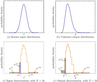
Our strategy (see Fig. 1) consists in three main steps and an optional fourth step.
1. FindNvalues of the random vectorX,
x1(1),...,xd(1),...,x1(N ),...,xd(N )
andN corresponding weights
w(1),...,w(N )
,
with PN
i=1w(i)=1, such that the discrete probability distributionfˆwhich assigns the weightw(i)to the point
x1(i),...,x(i)d (fori=1,...,N) is the optimal
approxi-mation off, among all the discrete probability distri-butions concentrated inNpoints. The meaning of opti-mality is to be precised later.
2. PerformNnumerical simulations to compute theN cor-responding valuesy(1),...,y(N )of the random variable
Y. We represent the action of the numerical code on the input data through a functionϕ, so that
y(i)=ϕx1(i),...,xd(i)fori=1,...,N.
3. Build a discrete approximationgˆofgby assigning the weightw(i)to the pointy(i)fori=1,...,N.
4. Usegˆto build a continuous probability distribution. The core of the problem is thus to find the “best” dis-cretization of a fixed continuous probability distribution f
(step 1). Stochastic quantization is a mathematical theory which allows to accomplish this task by giving a definition of the optimal discretization and providing an algorithm to find it. Once this is done, a discrete approximation of the un-known output probability distribution is automatically pro-duced (steps 2 and 3). Concerning step 3, it is a rigorous fact that the transformation of a discrete probability distribution by a functionϕ is the discrete probability distribution hav-ing the same weigths on the image points. Thus step 3 is the most natural choice. If we would know the output densityg, a better choice would be the weigths given by the SQ algo-rithm applied tog and the given output points. But we do not knowg. It is an open problem to improve step 3 in this direction.
Though the discrete probability distributiongˆcan be used to estimate the values of some parameters ofg(e.g. its mean, its variance, some quantiles), its graphical representation gives poor insight into the main qualitative features ofg. This is one of the motivations of step 4, which can be carried out through a kernel smoothing algorithm (e.g., Wand and Jones, 1995). Moreover, it may be useful for other purposes, like random number generation, to have a continuous distribution in output. The main idea of kernel smoothing algorithms is to smear out each weight w(i) around the corresponding pointy(i) according to a fixed rule and then to sum up all the contributions. This leads to the continuous probability distribution
ˆ
gKS(y)=
1
Nh
N X i=1
K y−y
(i)
h
!
!0.2 0 0.2 0.4 0.6 0.8 1 1.2 0
0.5 1 1.5 2 2.5 3 3.5 4 4.5
!00.2 0 0.2 0.4 0.6 0.8 1 1.2
0.5 1 1.5 2 2.5 3 3.5 4 4.5
x(1) x(10) y(1) y(10)
. . . . . . .. . .
w(1)
w(2)
w(10)
w(1)
w(2)
w(10)
x
x
y
y
probabilit
y
densit
y
probabilit
y
densit
y
probabilit
y
densit
y
probabilit
y
densit
y
(c) Input discretization, withN= 10. (c) Output discretization, withN= 10.
(a) Known input distribution. (b) Unknown output distribution.
Fig. 1. Graphical representation of the first three steps of our strategy, withd=1 andN=10. The lower graphs represent the discrete
approximations of the input and output probability distributions produced by the SQ method. The weightw(i)is the area of the rectangle
associated to thei-th point fori=1,...,N.
whereKis a smooth probability distribution andhis a mea-sure of the width of the interval over which each weight is spread. h is chosen according to an optimality criterion, based on the minimization of some kind of error resulting from the substitution ofgwithgˆKS. Kis usually chosen to be a unimodal probability density symmetric about zero, but its exact expression does not affect very much the result.
3 Quantization of univariate probability distributions (d=1)
As a first step, in order to give a precise meaning to the ex-pression “best approximation”, we introduce a distance be-tween probability distributions. Consequently, the optimal discretization off can be defined as the discrete probability distributionfˆwhich has the minimum distance fromf.
Since we have to compare discrete and continuous proba-bility distributions, it is easier to rely on the cumulative distri-bution functions, especially in the cased=1, in which there is only one input random variableX. LetF be the cumula-tive distribution function associated with the densityf and
ˆ
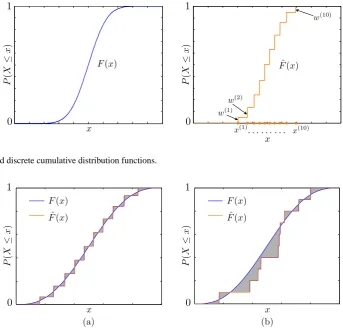
F the one associated withfˆ: namely (see Fig. 2),
F (x)=
Z x xmin
f (t )dt,
ˆ
F (x)= X
x(i)≤x ˆ
f x(i)= X
x(i)≤x
w(i),
forxmin≤x≤xmax,
wherexminandxmaxare the minimum and maximum values ofX,x(i)are the points in whichfˆis concentrated andw(i)
are the corresponding weights.
For instance, we can define a distance betweenf andfˆas
d(f,f )ˆ =
Z xmax
xmin
F (x)− ˆF (x)
dx (2)
(see Fig. 3). Therefore, the procedure consists in searching for the discrete probability distributionfˆwhich minimizes the quantityd(f,f )ˆ , among all the discrete distributions con-centrated inNpoints.
4 Quantization of multivariate probability distributions (d>1)
0 0.1 0.2 0.3 0.4 0.5 0.6 0.7 0.8 0.9 1 0
0.1 0.2 0.3 0.4 0.5 0.6 0.7 0.8 0.9 1
0 0.1 0.2 0.3 0.4 0.5 0.6 0.7 0.8 0.9 1
0 0.1 0.2 0.3 0.4 0.5 0.6 0.7 0.8 0.9 1
F(x) Fˆ(x)
x(1) x(10)
0 0
1 1
. . .. . .. . .
w(1) w(2)
w(10)
x
x
P
(
X
≤
x
)
P
(
X
≤
x
)
Fig. 2. Continuous and discrete cumulative distribution functions.
0 1
200 400 600 800 1000
0 0.2 0.4 0.6 0.8 1
x
P
(
X
≤
x
)
200 400 600 800 1000
0 0.2 0.4 0.6 0.8 1
0 1
P
(
X
≤
x
)
x
(a) (b)
F(x) F(x)
ˆ
F(x) Fˆ(x)
Fig. 3. The distance betweenf andfˆis defined as the shaded region area in the graphs. Optimal discrete distributions look like the one in graph (a), while graph (b) represents a sub-optimal discrete distribution.
probability density function ofX. IfX1,...,Xdare not inde-pendent, the probability density functionf (x1,...,xd)ofX is not related tof1(x1),...,fd(xd)in an obvious way. How-ever, the independency hypothesis is not necessary for the SQ algorithm.
A definition of distance similar to the one in Eq. 2 could be given, but it is easier and more appropriate to use another definition of distance, based on the random variables rather than on their cumulative distribution functions.
LetXˆ be a discrete random vector with probability distri-butionfˆ, approximating the continuous random vectorX; it seems quite natural to choose, as a measure of the distance betweenf andfˆ, the mean value of the errorX− ˆX
result-ing from the substitution ofXwithXˆ:
d(f,f )ˆ =EhX− ˆX
i
. (3)
The distance defined by Eq. (3) could be computed numer-ically, but the calculation is easier and faster (especially in high dimension) via a MC method; Appendix A shows in de-tail how it can be performed. The MC simulations involved in the algorithm use only samples ofX andXˆ, which can be generated easily, and not samples ofY, whose generation
is out of reach. The randomness on the value of d(f,f )ˆ
(and, as a consequence, on the values of the “optimal” points
x(1),...,x(N )) due to the choice of a stochastic algorithm can
be made negligible, provided that the numberMof MC sim-ulations is large enough. Moreover, the stochastic algorithm easily provides the weightsw(1),...,w(N )(see Appendix A). In appendix A we also show that, for univariate distribu-tions, the distances in Eqs. (2) and (3) lead to the same opti-mal discretization: therefore the definition given by Eq. (3), besides having an intuitive motivation, is a natural general-ization of that given by Eq. (2).
5 Testing SQ in a simple case
In order to assess the quality of the approximation of the out-put probability distribution given by the SQ, we first consider a simple test case.
0 0.1 0.2 0.3 0.4 0.5 0.6 0.7 0.8 0.9 1 0
0.1 0.2 0.3 0.4 0.5 0.6 0.7 0.8 0.9 1
0 0.1 0.2 0.3 0.4 0.5 0.6 0.7 0.8 0.9 1 0
0.1 0.2 0.3 0.4 0.5 0.6 0.7 0.8 0.9 1
0 0.1 0.2 0.3 0.4 0.5 0.6 0.7 0.8 0.9 1 0
0.1 0.2 0.3 0.4 0.5 0.6 0.7 0.8 0.9 1
0 0.1 0.2 0.3 0.4 0.5 0.6 0.7 0.8 0.9 1 0
0.1 0.2 0.3 0.4 0.5 0.6 0.7 0.8 0.9 1
0 0.1 0.2 0.3 0.4 0.5 0.6 0.7 0.8 0.9 1 0
0.1 0.2 0.3 0.4 0.5 0.6 0.7 0.8 0.9 1
0 0.1 0.2 0.3 0.4 0.5 0.6 0.7 0.8 0.9 1 0
0.1 0.2 0.3 0.4 0.5 0.6 0.7 0.8 0.9 1
0 0.1 0.2 0.3 0.4 0.5 0.6 0.7 0.8 0.9 1 0
0.1 0.2 0.3 0.4 0.5 0.6 0.7 0.8 0.9 1
0 0.1 0.2 0.3 0.4 0.5 0.6 0.7 0.8 0.9 1 0
0.1 0.2 0.3 0.4 0.5 0.6 0.7 0.8 0.9 1
true quantiles true quantiles
true quantiles
estimated
quan
tiles
estimated
quan
tiles
estimated
quan
tiles
0 0
0 0
0
0
1 1
1
1
1 1
N= 5 N= 10 N= 15
N= 20 N= 25 N= 30
N= 40 N= 50
percentiles percentiles percentiles
percentiles percentiles percentiles
percentiles percentiles
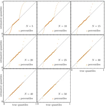
Fig. 4. Quantile-quantile plots. On the x-axis there are the true values of the quantiles ofg, on the y-axis their estimates given by the SQ.
The orange daggers represent the percentiles, from 1 to 99. If a dagger is close to the dashed liney=x, the SQ gives a good estimate of the
corresponding percentile. Different graphs refer to different numerosities of the SQ.
deviation 0.2, that ofX2has mean 0.6 and standard de-viation 0.1.
– The relation betweenXand the output random variable
Y is known and has a simple analytical expression:
Y =ϕ(X1,X2)
=1 8(X
2
1+X1)(X22+X2)+ 1
4(X1+X2). (4) In such a simple case it is possible to implement a MC method with very high numerosity (e.g. 105), producing an estimate ofgwhich can be considered exact for practical pur-poses. This version ofgcan be directly compared to the re-sults produced by the SQ method and by MC methods with variable numerosity, in order to establish which one gives the best approximation ofg: for instance, the SQ method can be compared to a MC with the same numerosity, or to other low numerosity MC simulations. For each numerosity, the MC can be repeated several times, thanks to the simplicity of the
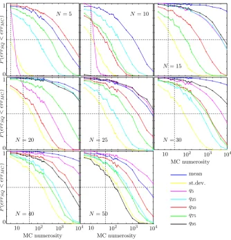
functionϕ; consequently, it is possible to estimate the prob-ability that the performances of the SQ are better than those of the MC (see Fig. 5).
Figure 4 compares some quantiles ofg, whose values are very well known thanks to the high numerosity MC, to their estimates produced by the SQ method. These estimates are obtained via a linear interpolation of the cumulative distribu-tion associated togˆ. Figure 4 shows that, as the numerosity
5 10 20 50 100 200 500 10002000 500010000 0 0.1 0.2 0.3 0.4 0.5 0.6 0.7 0.8 0.9 1
5 10 20 50 100 200 500 10002000 500010000 0 0.1 0.2 0.3 0.4 0.5 0.6 0.7 0.8 0.9 1
5 10 20 50 100 200 500 1000 2000 500010000 0 0.1 0.2 0.3 0.4 0.5 0.6 0.7 0.8 0.9 1
5 10 20 50 100 200 500 10002000 500010000 0 0.1 0.2 0.3 0.4 0.5 0.6 0.7 0.8 0.9 1
5 10 20 50 100 200 500 1000 2000 500010000 0 0.1 0.2 0.3 0.4 0.5 0.6 0.7 0.8 0.9 1
5 10 20 50 100 200 500 1000 2000 500010000 0 0.1 0.2 0.3 0.4 0.5 0.6 0.7 0.8 0.9 1
5 10 20 50 100 200 500 1000 2000 500010000 0 0.1 0.2 0.3 0.4 0.5 0.6 0.7 0.8 0.9 1
5 10 20 50 100 200 500 10002000 500010000 0 0.1 0.2 0.3 0.4 0.5 0.6 0.7 0.8 0.9 1 0 0 0 1 1 1
10 102 103 104 10 102 103 104
10 102 103 104
MC numerosity P ( er rSQ < er rMC ) P ( er rSQ < er rMC ) P ( er rSQ < er rMC ) MC numerosity MC numerosity mean st.dev. q5 q25 q50 q75 q95
N= 5 N= 10
N= 20 N= 25 N= 30
N= 40 N= 50
N= 15
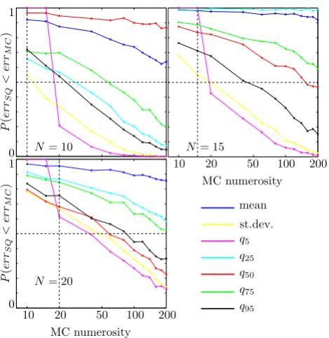
Fig. 5. Comparison between the SQ and MC simulations. On thexaxis there is the numerosity of the MC, in logarithmic scale; on the
yaxis there is the probability that errSQ<errMC, where errSQ=
p−pSQ
and errMC=
p−pMC
,pis the real value of a parameter of the
output probability distributiong,pSQandpMCare its estimates given by SQ and MC, respectively. The curves represent the results for
various parameters: mean, standard deviation and the 5%, 25%, 50%, 75%, 95% quantiles. The horizontal dashed line marks the value 0.5
of probability. Different graphs refer to different values of the numerosityNof the SQ. In each graph, a vertical dashed line is drawn in
correspondance of the MC numerosity equal toN.
However, Fig. 5 also shows that there is a general tendency to improvement asN grows. The whole bundle of curves, in fact, moves gradually towards the upper right corner of the graph: this means that the probability of the estimates given by the SQ being better than those given by the MC is gener-ally increasing asN grows. Furthermore, it is evident that, ifNis sufficiently high (N >10 in this case), the SQ method gives better results than MC simulations with the same nu-merosity with probability greater than 0.5.
6 Application of SQ to volcanic conduit dynamics
As a test application of the SQ approach to a volcanologically relevant case, we consider a one dimensional steady model of magma flow in a cilindrical conduit with fixed diameter and uniform temperature (Papale, 2001). This model is ideal for
testing SQ, since it provides a set of volcanologically rele-vant, strongly non-linear equations relating input and output distributions in a complex, unpredictable way, despite keep-ing the computational time small enough (order of minutes for each simulation) to allow a MC simulation withN=103. The output distribution given by this MC is reasonably close to the exact one and can be used for comparison with SQ. Hence, this first application of SQ to a volcanologically rele-vant case is also a further test of the method.
Among the several input quantities that are intrinsically uncertain we choose two of them, namely, the diameterDof the conduit and the total mass fraction of waterwH20. These
two quantities are known to largely control the conduit flow dynamics and the associated mass flow-rate (e.g., Wilson et al., 1980; Papale et al., 1998). D andwH20 are therefore
5 6 7 8 9 10 0
0.1 0.2 0.3 0.4 0.5 0.6 0.7 0.8 0.9 1
probabilit
y
densit
y
probabilit
y
densit
y
probabilit
y
densit
y
5 6 7 8 9 10
log10!m(kg/s)˙ " 20
70 120 20
70 120
0.5
9.5
5 5
9.5
0.5
D(m ) D(m
) wH2O(%)
wH2O(%)
MC N= 20 N= 15 N= 10
5 6 7 8 9 10
0 0.1 0.2 0.3 0.4 0.5 0.6 0.7 0.8 0.9 1
5 6 7 8 9 10
0 0.1 0.2 0.3 0.4 0.5 0.6 0.7 0.8 0.9 1
5 6 7 8 9 10
0 0.1 0.2 0.3 0.4 0.5 0.6 0.7 0.8 0.9 1
(b)
(c)
(d) (a)
5 6 7 8 9 10
0 1 0 0 1 1
x N= 10
N= 15
N= 20
P
! log
10
! ˙m
(kg/s)
" ≤
x
"
P
! log
10
! ˙m
(kg/s)
" ≤
x
"
P
! log
10
! ˙m
(kg/s)
" ≤
x
" MC
MC MC
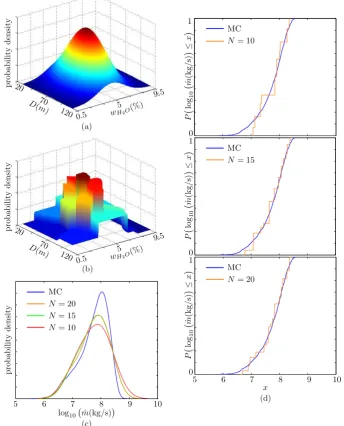
Fig. 6. Graph (a) represents the probability distribution of the input random vectorD,wH2O
, while in graph (b) there is its discretization
produced by the SQ withN=20. Graph (c) shows a comparison between the approximation ofgresulting from 103MC simulations andgˆKS,
which is obtained through the application of a kernel smoothing algorithm to the discrete distributiongˆgiven by the SQ withN=10,15,20.
Graph (d) represents a comparison between the cumulative distribution function resulting from 103MC simulations and those resulting from
the SQ withN=10,15,20, without application of kernel smoothing.
corresponding probability distribution of the logarithm of the mass-flow ratem˙. The latter is a volcanologically relevant quantity, as it defines the intensity of an eruption and as it largely affects the impact on the surroundings (Valentine and Wohletz, 1989; Todesco et al., 2002).
Figure 6a shows the assumed continuous distribution of the two random variableswH20andD, while Fig. 6b
illus-trates the result of the application of the SQ method to dis-cretize the distribution in 20wH20-Dpairs. In order to test
the SQ method, the discretization has been done also with
15 and 10wH20-Dpairs. The results have been compared, in
terms of output probability density (Fig. 6c) and cumulative probability distribution (Fig. 6d).
6 7 8 9 6
7 8 9
6 7 8 9
6 7 8 9
6 7 8 9
6 7 8 9
estimated
quan
tiles
N= 10 N= 15 N = 20
6 9
7 8
6 7 8 96 7 8 96 7 8 9
MC quantiles MC quantiles MC quantiles
percentiles percentiles percentiles
Fig. 7. Quantile-quantile plots, analogous to Fig. 4. On the x-axis there are the estimates of the quantiles ofggiven by a MC simulation with
N=103, which are close to the true values.
10 20 50 100 200 0
0.1 0.2 0.3 0.4 0.5 0.6 0.7 0.8 0.9
1 0 10 20 50 100 200
0.1 0.2 0.3 0.4 0.5 0.6 0.7 0.8 0.9 1
10 20 50 100 200 0
0.1 0.2 0.3 0.4 0.5 0.6 0.7 0.8 0.9 1
0 0 1
1
MC numerosity
P
(
er
rSQ
<
er
rMC
)
P
(
er
rSQ
<
er
rMC
) MC numerosity
mean st.dev. q5
q25
q50
q75
q95
N= 10
N= 20
N= 15
10 20 50 100 200
10 20 50 100 200
Fig. 8. Comparison between the SQ and MC simulations, analogous
to Fig. 5.
On the contrary, the left tail of the distribution, correspond-ing to the minimum mass flow-rates, is predicted accurately by the SQ. The improvement due to increased numerosity of SQ from 10 to 20 is clearly visible from the cumulative plots in Fig. 6d.
Figure 7 compares the estimates of the quantiles of the out-put distribution of mass flow-rates given by MC and SQ with
N=10, 15 and 20. The quantiles are obtained by means of a linear interpolation of the cumulative distributions in Fig. 6d. As for the analogous Fig. 4 (referring to the polynomial map at Eq. 4), the bulk of the distribution is predicted well by the SQ method, but the tails of the distribution are not. While a significant improvement clearly emerges from N=10 to
N=15, there is no significant gain in accuracy when moving
Table 1. Comparison between the estimates of some parameters of
the output distribution given by the SQ withN=10,15,20 points
and by a MC with 103simulations. The considered parameters are
the mean, the standard deviation and the 5%, 25%, 50%, 75%, 95% quantiles.
mean st. dev. q5 q25 q50 q75 q95
MC 7.74 0.50 6.71 7.45 7.86 8.12 8.38 SQ,N=10 7.75 0.41 7.09 7.32 7.86 8.07 8.32 SQ,N=15 7.74 0.44 6.94 7.46 7.82 8.10 8.33 SQ,N=20 7.73 0.46 6.85 7.49 7.79 8.09 8.35
fromN=15 toN=20. Table 1 shows the same results nu-merically for a few selected quantiles.
As for the ideal case discussed above, it is possible to com-pare the performances of the SQ with those of some low nu-merosity MC simulations (Fig. 8). This time, the discrete distributions generated by the SQ and by the low numeros-ity MC simulations are both compared to the one obtained from the MC simulation withN=103. In all cases, and for any quantity investigated, the SQ provides a better approxi-mation of the output distribution than the MC with equal nu-merosity. For many quantities a MC with at least hundreds of simulations is required in order to exceed the accuracy given by SQ simulations with numerosity up to 20.
7 Conclusions
provides substantially better estimates of output distributions than the MC method with the same number of simulations. This property is already clear with values ofN around 15– 20, and it becomes stronger with the increase ofN. The re-sults are less definite for very smallN, likeN=5 and some-times 10, where further ideas and research are needed. In general, MC gives results comparable to SQ only when the number of MC simulations is much higher, sometimes by one or more orders of magnitude, than that of SQ. Therefore, the SQ method results in a considerable computational sav-ing for the same degree of accuracy of the estimates. With values ofN of 15 or 20, in general the estimates obtained by SQ are very close to the true ones (or to our better estimates of the true ones).
In conclusion, the SQ method allows the introduction of uncertainties in the deterministic approach without requiring exceeding CPU time. This result is promising for the capa-bility of estimating future volcanic scenarios and volcanic hazards by means of a merged deterministic-probabilistic approach, whereby complex deterministic models are em-ployed by taking into account the intrinsic uncertainties in-volved in the definition of the conditions characterizing the volcanic systems.
Appendix A
The numerical algorithm
This appendix describes in detail how the distanced(f,f )ˆ, defined in Eq. (3), is approximately computed via a stochastic algorithm. Morevorer, it shows that the op-timal discretization of f is found by moving the points
x(1),...,x(N )in such a way thatd(f,f )ˆ is minimized, i.e. by
minimizing a function ofN d-dimensional vectors (function
hin Eq. A3 below).
The starting point is represented by a fundamental result of the SQ theory (Graf and Luschgy, 2000, Lemma 3.1), which states that, if theN possible values
x1(1),...,xd(1),...,x1(N ),...,xd(N )
of the random vectorXˆ, i.e. theN points in whichfˆis con-centrated, are fixed, then the corresponding optimal weights
w(1),...,w(N )are uniquely determined.
More precisely, the weights are defined as follows. – Fori=1,...,N, letVibe the region of thed-dimensional
space such that
x∈Vi⇐⇒
x−x
(i)
=mink=1,...,N x−x
(k) ,
where x(k)=x(k)
1 ,...,x
(k) d
for k=1,...,N. Vi is
called the Voronoi region of x(i) with respect to the
set x(1),...,x(N ) ; it contains the points which are
closer to x(i) than to any other element of the set
x(1),...,x(N ) (see figure A1).
– The optimal approximationXˆ of the random vectorX is defined as follows:Xˆ=x(i)if and only if the value of
Xbelongs toVi. Namely,Xˆ is obtained by rounding off
Xto the nearest vector amongx(1),...,x(N ).
– Correspondingly,w(i)(i.e. the probability thatXˆ=x(i)) is the weight assigned toVi by the probability distribu-tionf:
w(i)=
Z Vi
f (x)dx.
IfXˆ is defined as just described, it can be shown (Graf and Luschgy, 2000, Lemma 3.4) that, in the cased=1,
E h
|X− ˆX|i=
Z xmax
xmin
F (x)− ˆF (x)
dx;
moreover, ifXˆ0 is another random variable, with the same possible values x(1),...,x(N ) but defined in whatever way, andFˆ0is its cumulative distribution function, it can be shown that
E h
|X− ˆX0|
i
≥
Z xmax
xmin
F (x)− ˆF0(x)
dx (A1)
≥
Z xmax
xmin
F (x)− ˆF (x)
dx=E
h
|X− ˆX|i.
This means that, in the case d=1, minimizing
Rxmax
xmin
F (x)− ˆF (x)
dx is the same as minimizing E
h
|X− ˆX|i, so that the criterion used when there are several parameters in input is indeed a generalization of that used when there is only one parameter.
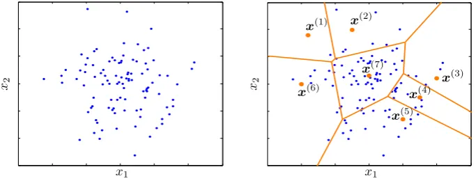
If the points x(1),...,x(N )are fixed, an approximate cal-culation of the minimum value of the distance in Eq. (3) and of the corresponding optimal weights w(1),...,w(N )can be carried out through the following steps (see Fig. A1):
1. generate a large number M (e.g. M=105) of d -dimensional random vectorsz1,...,zMwith probability distributionf;
2. for each vectorzj, select the indexij such thatzj be-longs toVij, i.e.
zj−x
(ij)
=mink=1,...,N zj−x
(k) ;
3. fork=1,...,N, assign tox(k)the weight
w(k)=m
(k)
0.2 0.3 0.4 0.5 0.6 0.7 0.8 0.2
0.3 0.4 0.5 0.6 0.7 0.8
0.2 0.3 0.4 0.5 0.6 0.7 0.8 0.2
0.3 0.4 0.5 0.6 0.7 0.8
x1 x1
x2 x2
x(1) x(2)
x(3) x(4) x(5) x(6)
x(7)
Fig. A1. Implementation of the stochastic quantization method withd=2 andN=7. The blue points are a sample of the input random
vectorX=(X1,X2); the orange pointsx(1),...,x(7)are the possible values ofXˆ, which is a discrete approximation ofX. The orange lines
define the Voronoi regions generated by the setnx(1),...,x(7)o: the region associated tox(i)contains the sample points which are closer to
x(i)than to any other of the orange points.
wherem(k)is the number of vectorszj into the Voronoi regionVk, i.e. the number of indexesj such thatij=k; 4. calculate
d(f,f )ˆ =E
h X− ˆX
i
≈ 1
M
M X j=1
zj−x(ij)
. (A2)
In our situation, in which the points(x(1),...,x(N ))are not fixed, the function
h
x(1),...,x(N )= 1
M
M X j=1
zj −x(ij)
(A3)
must be minimized. The minimization is performed using Powell’s method (Powell, 1964; Press et al., 2001), which moves the pointsx(1),...,x(N ), starting from an initial guess; for each new choice ofx(1),...,x(N ), the algorithm evaluates
h x(1),...,x(N )
going through the steps 1–4 above. The set of points which produces the minimum value ofhis just the optimal set of points we are searching for. In order to min-imize the risk of finding local minima, the minimization is repeated 10 times, varying the initial guesses, and the lowest minimum is taken as the best estimate of the true minimum.
Note that the error in the estimate (Eq. A2) ofd(f,f )ˆ is proportional to √1
M, so that, for sufficiently high values of
M, it becomes negligible and minimizing 1
M
M X j=1
zj−x(ij)
is the same as minimizingd(f,f )ˆ.
Acknowledgements. The authors are grateful to two anonymous
referees whose careful reading of the submitted paper contributed to improve its clarity.
Edited by: R. Moretti
References
Bennett, W. R.: Spectra of quantized signals, Bell Syst. Tech. J., 27, 446–472, 1948.
Currin, C., Mitchell, T. J., Morris, M., and Ylvisacker, D.: Bayesian prediction of deterministic functions with applications to the de-sign and analysis of computer experiments, J. Am. Stat. Assoc., 86, 953–963, 1991.
Graf, S. and Luschgy, H.: Foundations of quantization for probabil-ity distributions, Springer-Verlag, Berlin-Heidelberg, 2000. Gray, R. M. and Neuhoff, D. L.: Quantization, IEEE T. Inform.
Theory, 44(6), 2325–2383, 1998.
Kennedy, M. C. and O’Hagan, A.: Bayesian calibration of computer models, J. Roy. Stat. Soc. B, 63, 425–464, 2001.
Neri, A., Esposti Ongaro, T., Menconi, G., De’ Michieli Vitturi, M., Cavazzoni, C., Erbacci, G., and Baxter, P. J.: 4D simulation of explosive eruption dynamics at Vesuvius, Geophys. Res. Lett., 34, L04309, doi:10.1029/2006GL028597, 2007.
Oliver, B. M., Pierce, J. and Shannon, C. E.: The philosophy of PCM, P. IRE, 36, 1324-1331, 1948.
Panter, P. F. and Dite, W.: Quantizing distortion in pulse-count mod-ulation with nonuniform spacing of levels, P. IRE, 39, 44–48, 1951.
Papale, P., Neri, A., and Macedonio, G.: The role of magma compo-sition and water content in explosive eruptions, 1. Conduit ascent dynamics, J. Volcanol. Geoth. Res., 87, 75–93, 1998.
Papale, P.: Dynamics of magma flow in volcanic conduits with variable fragmentation efficiency and nonequilibrium pumice de-gassing, J. Geophys. Res., 106, 11043–11065, 2001.
Powell, M. J. D.: An efficient method for finding the minimum of a function of several variables without calculating derivatives, Comput. J., 7, 155–162, 1964.
Press, W. H., Teukolsky, S. A., Vetterling, W. T., and Flannery, B. P.: Numerical Recipes in Fortran 77, Cambridge University Press, Cambridge, 2001.
Sacks, J., Welch, W. J., Mitchell, T. J., and Wynn, H. P.: Design and analysis of computer experiments, Stat. Sci., 4, 409–435, 1989. Sparks, R. S. J.: Forecasting volcanic eruptions, Earth Planet. Sc.
Todesco, M., Neri, A., Esposti Ongaro, T., Papale, P., Macedo-nio, G., Santacroce, R., and Longo, A.: Pyroclastic flow haz-ard assessment at Vesuvius (Italy) by using numerical modelling: I. Large-scale dynamics, B. Volcanol., 64, 155–177, 2002. Valentine, G. A. and Wohletz, K. H.: Numerical models of Plinian
eruption columns and pyroclastic flows, J. Geophys. Res., 94, 1867–1887, 1989.
Wand, M. P. and Jones, M. C.: Kernel smoothing, Chapman and Hall, Boca Raton, 1995.