www.nonlin-processes-geophys.net/15/915/2008/ © Author(s) 2008. This work is distributed under the Creative Commons Attribution 3.0 License.
Nonlinear Processes
in Geophysics
Structure function analysis and intermittency in the atmospheric
boundary layer
J. M. Vindel1, C. Yag ¨ue2, and J. M. Redondo3 1Agencia Estatal de Meteorolog´ıa, Madrid, Spain
2Dept. Geof´ısica y Meteorolog´ıa, Universidad Complutense de Madrid, Spain 3Dept. F´ısica Aplicada, Universidad Polit´ecnica de Catalu˜na, Barcelona, Spain
Received: 10 April 2008 – Revised: 31 July 2008 – Accepted: 1 October 2008 – Published: 27 November 2008
Abstract. Data from the SABLES98 experimental campaign (Cuxart et al., 2000) have been used in order to study the relationship of the probability distribution of velocity incre-ments (PDFs) to the scale and the degree of stability. This connection is demonstrated by means of the velocity struc-ture functions and the PDFs of the velocity increments.
Using the hypothesis of local similarity, so that the third order structure function scaling exponent is one, the inertial range in the Kolmogorov sense has been identified for dif-ferent conditions, obtaining the velocity structure function scaling exponents for several orders. The degree of intermit-tency in the energy cascade is measured through these expo-nents and compared with the forcing intermittency revealed through the evolution of flatness with scale.
The role of non-homogeneity in the turbulence structure is further analysed using Extended Self Similarity (ESS). A criterion to identify the inertial range and to show the scale independence of the relative exponents is described. Finally, using least-squares fits, the values of some parameters have been obtained which are able to characterize intermittency according to different models.
Correspondence to: J. M. Vindel ([email protected])
1 Introduction
The single point velocity structure function of orderp, for a certain temporal scale (τ),is defined as:
Sp(τ )=|u(t+τ )−u(t )|p (1)
Richardson (1922) assumed the existence of an energy cas-cade, which was formalized along the so-called inertial range by Kolmogorov (1941, 1962). The spatial and temporal de-scriptions of the cascade may be exchanged assuming Tay-lor’s “frozen eddy” hypothesis (Stull, 1988), but care is needed in non-homogeneous flows (Mahjoub et al., 1998). Within the inertial range, for homogeneous and isotropic tur-bulence in local equilibrium, Kolmogorov (1941) established the following relation between the spatial structure functions and length scales (l):
Sp(l)∼ hεip/3lp/3 (2)
wherehεiis the mean energy dissipation rate assuming that it does not vary in space or time. This inertial range spreads out from the integral scale (of the order of the scale which generates the perturbation) to the Taylor microscale (of the three standard turbulence length scales, the one for which viscous dissipation begins to affect the eddies) and contin-ues further to smaller scales defined by Kolmogorov (the scale that characterizes the smallest dissipation-scale eddies; Glickman, 2000).
Whether we consider spatial or time dependence, if the conditions of existence of an equilibrium inertial range are satisfied, a potential type relationship is observed between the structure functions or different order, p, and the scale (e.g. Anselmet et al., 1984, for shear flows):
Sp(τ )∼τζp (3)
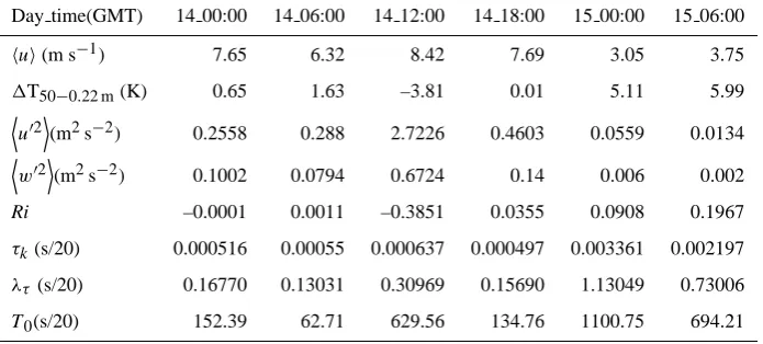
Table 1. Micrometeorological variables for the different situations (z=32 m): mean wind speed (hui), inversion strength (1T50−0.22 m),
wind speed varianceDu02 E
, vertical wind speed varianceDw02 E
, gradient Richardson number (Ri), Kolmogorov scale (τk), Taylor scale
(λτ)and time integral scale (T0).
Day time(GMT) 14 00:00 14 06:00 14 12:00 14 18:00 15 00:00 15 06:00
hui(m s−1) 7.65 6.32 8.42 7.69 3.05 3.75
1T50−0.22 m(K) 0.65 1.63 –3.81 0.01 5.11 5.99 D
u02E(m2s−2) 0.2558 0.288 2.7226 0.4603 0.0559 0.0134
D
w02E(m2s−2) 0.1002 0.0794 0.6724 0.14 0.006 0.002
Ri –0.0001 0.0011 –0.3851 0.0355 0.0908 0.1967
τk(s/20) 0.000516 0.00055 0.000637 0.000497 0.003361 0.002197 λτ(s/20) 0.16770 0.13031 0.30969 0.15690 1.13049 0.73006 T0(s/20) 152.39 62.71 629.56 134.76 1100.75 694.21
whereζp is the so-called scaling exponent, now defined in time, but with the same value as the spatial ones, provid-ing Taylor’s hypothesis holds (Stull, 1988). Willis and Dear-dorff (1976) showed that in order to satisfy the requirement for the eddy to have negligible change as it advects past a sensor, the wind standard deviation should be less than half the value of wind speed, and this condition is fulfilled by our data.
According to Kolmogorov’s (1941) initial theory, the mean energy dissipation rate,hεi, along the different scales of the Richardson cascade was expected to remain constant. Kolmogorov established a linear dependence of the expo-nentsζp as a function of the orderp. However, experimen-tally, first Batchelor and Townsend (1949), and then Lan-dau (see LanLan-dau and Lifshitz, 1959; Frisch, 1995), observed deviations from Kolmogorov’s theory. This phenomenon is generally known as intermittency of the turbulence cascade, and is characterized by the anomalous scaling exponents (deviations from the exponents ζp=p/3 foreseen by Kol-mogorov, 1941). In a more refined theory, assuming a log-normal variation, Kolmogorov (1962) introduced the possi-bility of scale dependence of dissipation, which sparked a wealth of different phenomenological models of turbulence, (see Frisch, 1995, for an historical account) that give sev-eral approximations to these exponents. Other methods try to derive intermittency directly from Navier-Stokes equations (see, e.g., Grossmann et al., 1994; Giles, 2001; or more re-cently, Angheluta et al., 2006, for the case of a nonlinear model of turbulence).
The local dissipation hεi=
υωijωj i, with υ the kinematic viscosity and ω the vorticity so that ωij=(∂ui/∂xj−∂uj/∂xi) is generally a very complicated (multifractal) function. When the local energy dissipation is not constant with the scale, it is said that intermittency
is present, but we should note that we may be including other effects, such as non-homogeneity or anisotropy, within a single concept. The probability distribution of ε (or of other variables dependent on the scale, as is the case with the velocity or temperature increments or their derivatives) will differ according to the scale taken into account. In the range between the integral scale, L0, (the scale of the order of disturbance generated by the turbulence) and the Taylor microscale, (where production and dissipation are in equilibrium) which we will call macroturbulence (Rodriguez et al., 1999), the corresponding normalized PDF usually appears Gaussian and, as a result of intermittency, modifies its shape more and more as the scale diminishes (see, e.g. Biferale, 1993; Li and Meneveau, 2005; or Li and Meneveau, 2006).
Thus, an index that characterizes the variation of proba-bility distribution could be introduced as an intermittency index (of macroturbulence) related to flatness or Kurtosis. For example, Chevillard et al. (2005), considered the direct measure of log F3
, where F is the flatness of the veloc-ity. Bottcher et al. (2007) have recently shown an exam-ple of the evolution of flatness with scale: for large scales, the flatness has values around 3 (Gaussian flatness), and it increases as the PDF appears more and more pointed. An-other method of characterizing the intermittency of the cas-cade in the Kolmogorov (1962) sense is to measure the dif-ference between 2 and the sixth order scaling exponent of the structure function,µ=2−ζ6, but we should observe that this simply includes in a single parameter the many possi-ble deviations from the Kolmogorov (1941) result (ζp=p/3), including non-homogeneity and non-locality.
In this article, both indices of intermittency (scaling ex-ponents and variation of flatness) will be measured for at-mospheric boundary layer velocity data and related and,
18
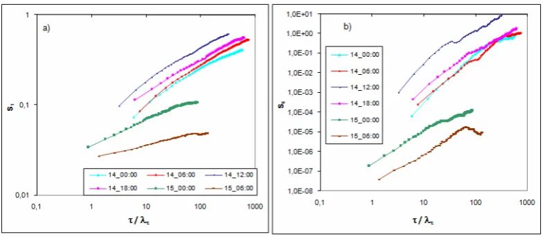
Figure 1: Evolution of the structure functions with the scale for different stratification
situations. a) order 1; b) order 6.
Fig. 1. Evolution of the structure functions with the scale for different stratification situations. (a) order 1; (b) order 6.
although with the present data it is not possible to establish a univocal correlation between the type of stratification and the degree of existing intermittency, a stronger dependence is found between the type of stratification and the structure functions. First we present the data, followed by the PDF and structure functions analysis, a statistical convergence study, the flatness and scaling exponents results, and finally the ap-plication of Extended Self Similarity and some other inter-mittent scaling theories.
2 Data
SABLES98 (Stable Atmospheric Boundary Layer Experi-ment in Spain 1998) data (Cuxart et al., 2000) from a sonic anemometer (20 Hz sampling rate) at 32 m were used. This field campaign took place in September 1998 (from 10 to 28) at the Research Centre for the Lower Atmosphere (CIBA) which is situated on the Northern Spanish Plateau. The sur-rounding terrain is fairly flat and homogeneous. In the exper-iment, different degrees of stable stratification were achieved during the night, from near-neutral to very stable conditions. The analysis presented here was done for six differ-ent stability situations (with a temporal lag of 6 h) be-tween 14 September at 00:00 GMT and 15 September at 06:00 GMT. Accordingly, this work examines not only noc-turnal data, but also diurnal situations where convective in-stability was present. Turbulent and in-stability parameters as well as mean wind speed can be found in Table 1, although further information can be found in Yag¨ue et al. (2006).
A bulk index of the existing stability degree in each situa-tion is the difference of temperature between the levels of 50 and 0.22 m showing the strength of surface-based inversion developed during the night, or the convective lapse rate dur-ing the day. It is also important to measure the level of strati-fication by calculating the local gradient Richardson number. This non-dimensional number takes into account the local
vertical wind shear as well as the density gradient. In the tur-bulent kinetic energy equation, the Flux Richardson number is the ratio of the buoyancy and production terms, and relat-ing fluxes to gradients (Redondo et al., 1996) it is possible to measure Ri locally in general as:
Ri=g1ρL0/ρu02 (4)
where 1ρ is the density difference and L0 is the integral scale. From the actual measured temperature and horizon-tal velocity data, the gradient Richardson number is defined (Cuxart et al., 2000) as:
Ri= g θ0 ∂θ ∂z ∂u ∂z 2
+u2∂α∂z
2 (5)
To evaluate the gradients of wind velocity (u) and poten-tial temperature (θ), log-linear fits (Nieuwstadt, 1984) were made to the different levels data. The wind direction (α) gra-dient is evaluated using simple linear fits:
u=az+blnz+c θ=a0z+b0lnz+c0 α=a00z+c00
(6)
It may be established from Table 1 (where all the stabil-ity and turbulent parameters agree) that on 14 September at 12:00 GMT there was a clearly convective instability sit-uation, and that on 15 September at 06:00 GMT and at 00:00 GMT there occurred the most stable situations (higher inversion strengths and Richardson numbers, lower wind speeds and horizontal and vertical variances). However, smaller and less clear differences are found on 14 Septem-ber at 00:00 GMT, 06:00 GMT and 18:00 GMT: according to the Richardson number, 00:00 GMT is the most neutral sit-uation, while 06:00 GMT is the situation where vertical tur-bulent transfer is most inhibited (lower vertical covariance, lower wind speed and greater inversion strength).
19
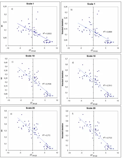
Figure 2: Order 1 structure function (left) and Standard deviation (right) versus
Δ
T50-0.22m
for a certain scale: a) and b): 1 (s/20); c) and d): 10 (s/20); e) and f): 20 (s/20) (Dots represent
conditions every 30 minutes) (Including the coefficient of determination corresponding to
least-squares linear fit).
Fig. 2. Order 1 structure function (left) and Standard deviation (right) versus1T50−0.22 mfor a certain scale: (a) and (b): 1 (s/20); (c) and
(d): 10 (s/20); (e) and (f): 20 (s/20) (Dots represent conditions every 30 minutes) (Including the coefficient of determination corresponding
to least-squares linear fit).
20
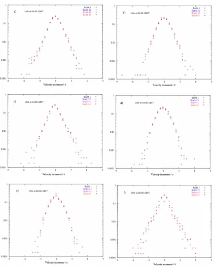
Figure 3: PDFs of velocity increments for different scales: a) the 14
that 00:00 GMT; b) the
14
that 06:00 GMT; c) the 14
that 12:00 GMT; d) the 14
that 18:00 GMT; e) the 15
that 00:00
GMT; f) the 15
that 06:00 GMT.
Fig. 3. PDFs of velocity increments for different scales: (a) the 14th at 00:00 GMT; (b) the 14th at 06:00 GMT; (c) the 14th at 12:00 GMT; (d) the 14th at 18:00 GMT; (e) the 15th at 00:00 GMT; (f) the 15th at 06:00 GMT.
Table 2. Estimated scale ranges (s/20) for the different situations analyzed.
Day Time (GMT) 14 00:00 14 06:00 14 12:00 14 18:00 15 00:00 15 06:00 Range (Kolm) [2–59] [2–81] [1–74] [3–14] Not possible Not possible
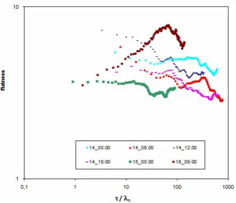
21 Figure 4: Evolution of flatness with scale for different stratification situations.
Fig. 4. Evolution of flatness with scale for different stratification
situations.
In Table 1 are included the typical Kolmogorov, Taylor and Integral scales, corresponding to the different situations. In the literature, to compare numerical simulations of turbu-lence, the scales are usually non-dimensionalized by Taylor’s scale, and in this work this has been done to compare differ-ent stability situations.
The Kolmogorov and Taylor spatial and temporal scales correspond to the following expressions (Tennekes and Lum-ley, 1994):
ηk=A(−1/4)Re(
−3/4) int L0≡
υ3 ε
!1/4
;τk= ηk
U (7)
λl= 15
A (1/2)
Re(int−1/2)L0; λτ= λl
U (8)
where A is a constant of the order of 1, which we will suppose equal to 0.5 (Balbastro et al., 2004), Reint is the Reynolds number corresponding to the integral scale (L0) andUis the wind speed.
Five-minute series (6000 data points) were used to study each situation, which is an optimal compromise between using enough data to provide the statistics and avoiding mesoscale motion influences, as we are interested in the tur-bulent scales (Stull, 1988).
In order to investigate the relationship between struc-ture functions and stability, five-minute series were anal-ysed every 30 min between 14 September (00:00 GMT) and 15 September (06:00 GMT). The variable studied was the horizontal velocity component in the mean flow direction (u), thus all further conclusions only apply to the horizon-tal structure of the boundary layer turbulence. It is clear that for less stratified turbulence the cascade will be more three-dimensional, while the reduction of the vertical scales below Ozmidov’s length scale as stratification increases will flatten Reynolds’ stresses in spite of a possible internal wave field.
3 Analysis of structure functions and PDFs
The potential relationship produced by Eq. (3) is shown in Fig. 1, where two structure functions (order 1 and order 6) have been represented for different situations. It is observed that by far the highest values for structure functions corre-spond to 14 September at 12:00 GMT, followed by the same day at 18:00 GMT and 06:00 GMT; then 14 September at 00:00 GMT and, finally, with values much lower than the previous ones, the situations represented for the 15th.
Higher values of structure functions imply a higher range for velocity increment values. That is to say, the dispersion of these increments is greater, due to a lack of homogene-ity. Structure functions and the degree of stratification must therefore present a certain relationship, as shown in Fig. 2, where an increase in the value of the structure functions may be observed (specifically ofS1 and standard deviation – square root ofS2– ), as the instability is increased (lower values in the temperature difference between the levels of 50 and 0.22 m.).
On the other hand, the phenomenon of intermittency al-ludes to infrequent events, which correspond to the veloc-ity increments furthest from zero. Thus the greater or lesser stretching of the tails in the PDFs is indicative of the (greater or lesser) grade of intermittency (Frisch, 1995; Sorriso-Valvo et al., 2000; Chevillard et al., 2006). In order to study these behaviour patterns, in Fig. 3 we have represented the PDFs (in log scale) of the velocity increments normalized by the Standard Deviation, corresponding to different scales and for the different situations. The following characteristics are ob-served:
1. The behaviour pattern of the scales, in a given situation, proves to be quite similar for the larger scales. The most
22
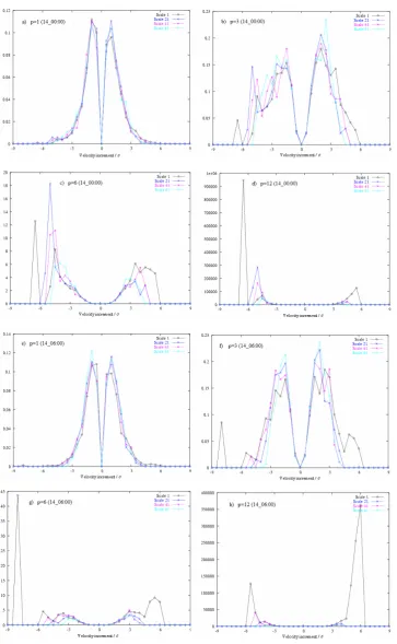
23 Figure 5: Product of the p-power (p=1, 3, 6 and 12) of the velocity increments by its corresponding probability versus the velocity increments for different scales: a) b) c) and d) for the 14th at 00:00 GMT; e), f) ,g) and h) for the 14th at 06:00 GMT.
Fig. 5. Product of thep-power (p=1, 3, 6 and 12) of the velocity increments by its corresponding probability versus the velocity increments for different scales: (a), (b), (c), and (d) for the 14th at 00:00 GMT; (e), (f), (g) and (h) for the 14th at 06:00 GMT.
24
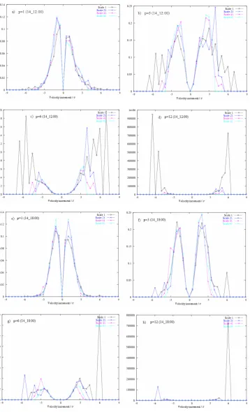
25 Figure 6: Product of the p-power (p=1, 3, 6 and 12) of the velocity increments by its corresponding probability versus the velocity increments for different scales: a) b) c) and d) for the 14th at 12:00 GMT; e), f) ,g) and h) for the 14th at 18:00 GMT.
Fig. 6. Product of thep-power (p=1, 3, 6 and 12) of the velocity increments by its corresponding probability versus the velocity increments for different scales: (a), (b), (c), and (d) for the 14th at 12:00 GMT; (e), (f), (g) and (h) for the 14th at 18:00 GMT.
26
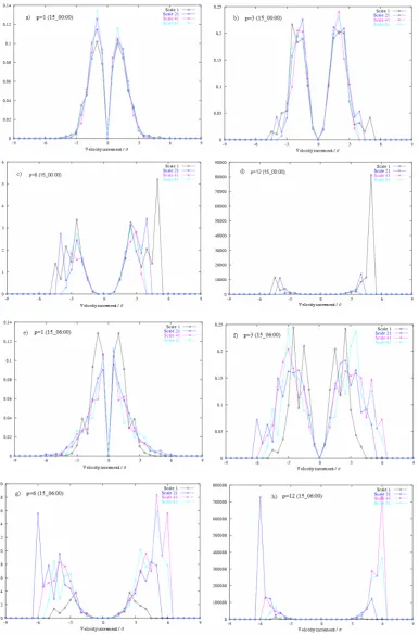
27 Figure 7: Product of the p-power (p=1, 3, 6 and 12) of the velocity increments by its corresponding probability versus the velocity increments for different scales: a) b) c) and d) for the 15th at 00:00 GMT; e), f) ,g) and h) for the 15th at 06:00 GMT.
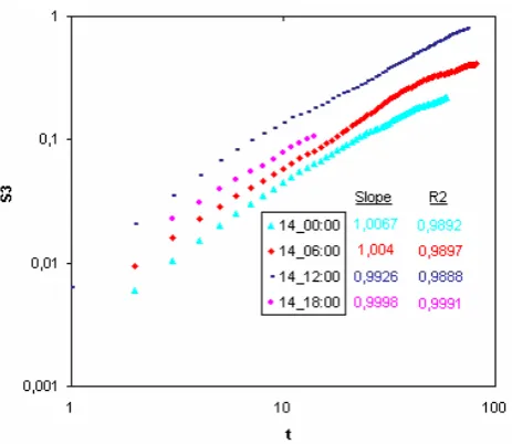
Figure 8: Slope of least-squares linear fit and coefficients of determination between log of the order 3 structure function and log of the scale for different stratification situations.
Fig. 7. Product of thep-power (p=1, 3, 6 and 12) of the velocity increments by its corresponding probability versus the velocity increments for different scales: (a), (b), (c), and (d) for the 15th at 00:00 GMT; (e), (f), (g) and (h) for the 15th at 06:00 GMT.
924 J. M. Vindel et al.: Atmospheric boundary layer intermittency
27 Figure 7: Product of the p-power (p=1, 3, 6 and 12) of the velocity increments by its corresponding probability versus the velocity increments for different scales: a) b) c) and d) for the 15th at 00:00 GMT; e), f) ,g) and h) for the 15th at 06:00 GMT.
Figure 8: Slope of least-squares linear fit and coefficients of determination between log of the order 3 structure function and log of the scale for different stratification situations.
Fig. 8. Slope of least-squares linear fit and coefficients of
determi-nation between log of the order 3 structure function and log of the scale for different stratification situations.
significant differences are appreciated in the tails of the smaller scales.
2. In Fig. 3b and c the tails of the smaller scales stretch further than in the other cases, indicative of a higher degree of intermittency. On the other hand, in Fig. 3e and f (the most stable situations) the tails of the smaller scales are more closed, especially in case 3f, where it may be seen that the PDF of scale 1 falls within the other PDFs.
The flatness of the PDFs shown above is statistically de-fined from the structure functions as:
F = S4
(S2)2
(9) As we have already said, flatness seems to be a very good indicator of the degree of existing intermittency: Biferale et al. (2008) point out that, when flatness changes with scale following a potential law, intermittency is present. Figure 4 shows, in log-log scale, the evolution of flatness with scale. It may be quite clearly seen that the greatest decrease of flat-ness with scale corresponds to 14 September at 12:00 GMT. However, the increase of flatness for the 15th at 06:00 GMT is particularly significant, in accordance with the closing of the PDFs for the smaller scales as mentioned above.
In order to show the degree of statistical convergence dis-played by the structure functions of the successive orders, we calculated for velocity increments, the product of the cor-responding probability by thep-power of those increments (Schumacher, 2001). The area below the curve thus obtained corresponds to the moment of order p and, consequently, the statistical convergence of that moment will improve when
28 Figure 9: Scaling exponents versus order of the structure function for different situations.
Figure 10: Structure functions of several orders (1, 6, 9 and 12) versus structure function of order 3 for the range below integral scale: a) for the 14th at 00:00 GMT; b) for the 15th at 00:00 GMT.
Fig. 9. Scaling exponents versus order of the structure function for
different situations.
the scatter of the curve decreases. In Figs. 5, 6 and 7 we have shown the curves mentioned above for orders 1, 3, 6 and 12 for the different situations analysed and various dif-ferent scales.
Certainly, for orders higher than 6 we may already observe a considerable scattering for certain values of the tails, which we consider satisfactory because with meteorological field data we are far from controlled laboratory wind tunnel con-ditions. The lack of strict statistical convergence for orders higher than 3 does not suppose any limitation to the method of analysis described here. On the other hand it stimulates the analysis of wind data at much higher frequency. Never-theless, because most of the data scattering and lack of con-vergence can be seen to take place fundamentally when the scale diminishes, at about the Taylor microscale, we may for-ward the hypothesis that the absence of convergence might be motivated by the existence of intermittence precisely in the non-equilibrium situations: stratified 2-D type turbulence and convective 3-D unstable situations. From our point of view the overall results of this work are relevant even if we limit the study to the smaller orders, where the convergence is much higher.
Figures 3, 4, 5, 6 and 7 prove to be convergent as to the possible intermittency shown by the different cases, with a very marked intermittency on the 14th at 12:00 GMT and the opposite result on the 15th, where there is considerable sta-bility.
J. M. Vindel et al.: Atmospheric boundary layer intermittency 925
28
Figure 9: Scaling exponents versus order of the structure function for different situations.
Figure 10: Structure functions of several orders (1, 6, 9 and 12) versus structure function of
order 3 for the range below integral scale: a) for the 14
that 00:00 GMT; b) for the 15
that
00:00 GMT.
Fig. 10. Structure functions of several orders (1, 6, 9 and 12) versus structure function of order 3 for the range below integral scale: (a) for
the 14th at 00:00 GMT; (b) for the 15th at 00:00 GMT.
29
Figure 11: Temporal evolution of absolute exponents (left) and absolute exponents
re-evaluated by the ESS method (right) for the first 6 structure functions for the different
situations: a) and b): 14
th_ 00:00 GMT; c) and d): 14
th_06:00 GMT.
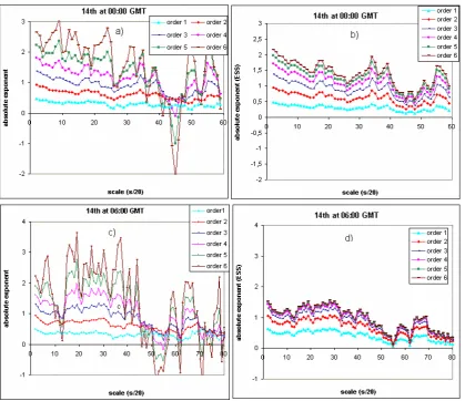
Fig. 11. Temporal evolution of absolute exponents (left) and absolute exponents re-evaluated by the ESS method (right) for the first 6
structure functions for the different situations: (a) and (b): 14th 00:00 GMT; (c) and (d): 14th 06:00 GMT.
30 Figure 12: Scaling exponents (ESS method) versus order of the structure function for different situations.
Fig. 12. Scaling exponents (ESS method) versus order of the
struc-ture function for different situations.
4 Determination of inertial range in the Kolmogorov sense
Table 1 shows the integral scales following the method of Van Fossen and Ching (1997) that reflects the upper scale of the inertial ranges corresponding to the different situations.
The empirical Kolmogorov 4/5 law establishes a relation-ship (for an incompressible flow in local equilibrium) be-tween the third order structure function and the spatial scale: S3(l)= −
4
5hεil (10)
This is a non-trivial result derived from Navier-Stokes equa-tions. The interval that verifies this law (Eyink, 2003) is con-ventionally considered as the inertial range. In this case, the scaling exponentsζp are constant along the whole interval, indicating not only homogeneity and isotropy but also local-ity of the cascade process. Gotoh (2001) confirmed that this law holds using DNS at high Reynolds numbers.
Table 2 shows a series of possible inertial ranges for the situations under study. They have been obtained assuming a slope equal to 1 in Fig. 8, which relates the logarithm of the structure function of order 3 with the logarithm of the scale. We see that there are situations, such as 15 September at 00:00 GMT and at 06:00 GMT, in which it is not possible to obtain this interval. The slopes for other orders p represent the scaling exponentsζp.
The estimators of these slopes,b∗, will be affected by the error produced when the points are fitted to a straight line by the least squares method. Thus, setting a certain valueγ for the confidence interval for the slopeb, it is possible to calculate the error interval forb∗. Comparing the relation-ship betweenζp andp withp/3 (values for the exponents
ζp, foreseen by the K41 theory), the degree of intermittency may be established (Fig. 9, where a 99% confidence interval has been chosen). The greater the deviation fromp/3, the greater the degree of intermittency in the cascade. Accord-ing to this, the situations, within their correspondAccord-ing inertial ranges of lesser to greater intermittency, are the following: on the 14th at 00:00 GMT, at 18:00 GMT, at 06:00 GMT and, with a slightly greater difference, at 12:00 GMT. This result agrees well with the conclusions that may be drawn from the previous figures, although these are not restricted to the iner-tial range evaluated in the Kolmogorov sense.
5 Inertial range determination by the Extended Self-Similarity method (ESS)
According to this method (Benzi et al., 1993), the inertial range is the interval where a potential relationship between the structure function and the structure function of order 3 is fulfilled:
SpαS3ζp (11)
The exponentsζp are called relative exponents and are con-stant for this inertial range. Their values are:
ζp=ζp/ζ3 (12)
Unlike the previous method, this one is not limited to homo-geneity intervals. Therefore, the scaling exponent, usually known as the absolute exponent (ζp), is not now constant throughout the inertial range.
Using structure functions up to degree 12, we have checked that Eq. (11) is verified for the ranges below inte-gral scale (Table 1), with a determination coefficient of at leastR2>0.85 for all cases (Fig. 10).
The ESS procedure seems more general, since it elimi-nates the requirement for the third order structure functions to be unity for the whole range. This behaviour is typical of stable strongly non-homogeneous flows, such as those on 15 September at 00:00 GMT and 06:00 GMT.
An estimate of absolute exponents for each scale was made, multiplying the corresponding constant relative expo-nent by the absolute expoexpo-nent of order 3. Figure 11a and c show a first approximation to the absolute exponents for each scale: the value of the absolute scaling exponents is the slope of the log. of the structure functions against the log. of the scales (the slopes are obtained for two consecutive points). In the segments where the absolute exponents de-crease, the relative exponents are almost constant (Mahjoub, 2000; Mahjoub et al., 1998, 2000, 2001). If these previous absolute exponents of order 3 are multiplied by the relative ones (corresponding to slopes of the log of the structure func-tions versus the log of structure funcfunc-tions of order 3), re-evaluated absolute exponents are obtained (Fig. 11b and d). In this figure, a similar shape is observed among all expo-nents for the different orders.
31
Figure 13: Scaling exponents versus order of the structure function obtained by different methods: a) 14 th_00:00 GMT; b) 14th_06:00 GMT; c) 14th_12:00 GMT; d) 14th _18:00 GMT.
Fig. 13. Scaling exponents versus order of the structure function obtained by different methods: (a) 14th 00:00 GMT; (b) 14th 06:00 GMT; (c) 14th 12:00 GMT; (d) 14th 18:00 GMT.
In the subranges where homogeneity holds, such as those previously evaluated, we may use the relative exponents ob-tained, which are then equal to the absolutes, to determine the intermittency (Fig. 12). The results are practically identi-cal to those obtained with the previous method, although the error bars are shorter, giving greater reliability to the results.
6 Fits from theoretical models
There are several models which seek to explain the pro-file that scaling exponents adopt when there is intermittency (Frisch, 1995). These models are characterized by one or more parameters whose values show the degree of intermit-tency.
For example, the binomial model (Meneveau and Sreeni-vasan, 1987): in the absence of intermittency the value of the intermittency parameter is 0.5; when intermittency increases, it also increases. The relationship between the parameter (m) and theporder scaling exponents is:
ζp=1−log2(mp/3+(1−m)p/3) (13) In the case of log-normal model (Kolmogorov, 1962), the intermittency parameter isµ(in the absence of intermittency, its value is 0; when intermittency increases, its value in-creases), being the relation betweenµand scaling exponents: ζp=
p 3 +
µp
18(3−p) (14)
Using a least-squares fit, the parameters able to character-ize intermittency according to the model (Fig. 13) have been estimated. We can see that the values of these parameters in-crease (from 0.5 for the binomial model and from 0, in the case of the log-normal model) as the degree of intermittency is greater, in accordance with the results shown above.
7 Summary and conclusions
We have performed a thorough analysis of the PDFs of the horizontal velocity differences for different atmospheric boundary layer situations and for different scales, and it has been seen the evolution of flatness with the scale, as well as that between structure functions and the degree of stratifica-tion.
In order to quantify these relationships, we adopted Kol-mogorov’s scaling to calculate the subrange where scaling exponents are constant. At the same time, using ESS we were able to recalculate the exponents (relative and absolute) for the same inertial subrange.
We have confirmed the applicability of the method, even if the resolution of the measurements only resolves the macro-turbulence characteristics between the integral length scale and the Taylor microscale, but we do not claim that the tur-bulence is (necessarily) under local equilibrium.
Finally, using least-squares fits, the values of the param-eters able to characterize the intermittency for the different stabilities, according to two different turbulence models (the binomial and the log-normal models) have been found.
We therefore highlight the following conclusions: – The relationship existing between the structure
func-tions and stratification shows that as stability increases the structure functions decrease.
– The variation of flatness (F )with scale shows (Fig. 4) that the most stable (15th 06:00 GMT) and unstable sit-uations (14th 12:00 GMT) have the highest values ofF, but it is very interesting to note that for stably stratified flows, this happens at large scales.
– The overall results show that for convective, unstable turbulence intermittency (µ) increases. On the other hand, neutral conditions exhibit low intermittency. – The determination of an inertial range in the
Kol-mogorov 1941 sense implies the identification of a ho-mogeneity interval, which, in situations of high stabil-ity, is not always possible (15 September at 00:00 and 06:00 GMT).
– Absolute exponents have been shown, and no clear re-lationship between the degree of intermittency and the type of stratification has been established. However, the relationship between three ways of describing the inter-mittency has been pointed out: the evolution of flatness with the scale, the evolution of PDFs with the scale and the values of the absolute scaling exponents.
– Re-evaluating absolute exponents using ESS for the dif-ferent orders, a more similar shape is observed among all exponents. Moreover, these re-evaluated exponents show a smoother shape than the initial exponents be-cause of the compensating effect described in Mahjoub
et al. (1998), and intermittency evaluated shows a higher degree of accuracy.
– The ESS method is applicable over the whole of the inertial subrange; but only within the subranges calcu-lated assuming homogeneity and Kolmogorov scaling it is possible to compare intermittency for different situa-tions. Otherwise we would need different intermittency parameters for each range of scales.
For strongly non-homogeneous flows, new types of intermit-tency parameters are needed that take into account the non-homogeneity and the non-locality of the turbulent cascades. Acknowledgements. This research has been funded by the Spanish
Ministry of Education and Science (projects ESP2005-07551, CGL 2004-03109 and CGL 2006-12474-C03-03). The IV PRICIT program (supported by CM and UCM) has also partially financed this work through the Research Group “Micrometeorology and Climate Variability” (No. 910437). We thank the referees for their suggestions.
Edited by: A. Baas
Reviewed by: two anonymous referees
References
Angheluta, L., Benzi, R., Biferale, L., Procaccia, I., and Toschi, F.: Anomalous scaling exponents in nonlinear models of turbulence, Phys. Rev. Lett., 97, 1–4, 2006.
Anselmet, F., Gagne, Y., Hopfinger, E. J., and Antonia, R. A.: High-order velocity structure functions in turbulent shear flows, J. Fluid Mech., 140, 63–89, 1984.
Balbastro, G. C., Sonzogni, V. E., Franck, G., and Storti, M.: Acci´on del viento sobre cubiertas abovedadas aisladas: sim-ulaci´on num´erica, Mec´anica Computacional Vol. XXIII, Bar-iloche, Argentina, November 2004.
Batchelor, G. K. and Townsend, A. A.: The nature of turbulent mo-tion at large wave numbers, Proc. Royal Soc. London A., 199, 238–255, 1949.
Benzi, R., Ciliberto, S., Tripiccione, R., Baudet, C., Massaioli, F., and Succi, S.: Extended self-similarity in turbulent flows, Physi-cal Review E., 48, R32, 1993.
Biferale, L.: Probability distribution functions in turbulent flows and shell models, Phys. Fluids A., 5, 428–435, 1993.
Biferale, L., Bodenschatz, E., Cencini, M., Lanotte, A. S., Ouel-lette, N. T., Toschi, F., and Xu, H.: Lagrangian structure func-tions in turbulence: A quantitative comparison between experi-ment and direct numerical simulation, Phys. Fluids, 20, 065103, doi:10.1063/1.2930672, 2008.
B¨ottcher, F., Barth, S., and Peinke, J.: Small and large scale fluc-tuations in atmospheric wind speeds, Stochastic environmental research and risk assessment, 21, 299–308, 2007.
Chevillard, L., Castaing, B., and L´evˆeque, E.: On the rapid increase of intermittency in the near-dissipation range of fully developed turbulence, Eur. Phys. J. B., 45, 561–567, 2005.
Chevillard, L., Castaing, B., L´evˆeque, E., and Arneodo, A.: Uni-fied multifractal description of velocity increments statistics in
turbulence: intermittency and skewness, Physica D.: Non linear Phenomena, 218, 77–82, 2006.
Cuxart, J., Yag¨ue, C., Morales, G., Terradellas, E., Orbe, J., Calvo, J., Fern´andez, A., Soler, M. R., Infante, C., Buenestado, P., Es-pinalt, A., Joergensen, H. E., Rees, J. M., Vil´a, J., Redondo, J. M., Cantalapiedra, I. R., and Conangla, L.: Stable atmo-spheric boundary-layer experiment in Spain (SABLES98): a re-port, Bound.-Lay. Meteor., 96, 337–370, 2000.
Eyink, G. L.: Local 4/5-law and energy dissipation anomaly in tur-bulence, Nonlinearity, 16, 137–145, 2003.
Frisch, U.: Turbulence, Cambridge University Press, England, 296 pp., 1995.
Giles, M. J.: Anomalous scaling in homogeneous isotropic turbu-lence, J. Phisics A.: Mathematical and General, 34, 4389–4435, 2001.
Glickman, Todd S.: Glossary of Meteorology, Second Edition, American Meteorological Society, Boston, 2000.
Gotoh, T.: Turbulence research at large Reynolds numbers using high resolution DNS, RIKEN Review, 40, 3–6, 2001.
Grossmann, S. and Lohse, D.: Scale resolved intermittency in tur-bulence, Phys. Fluids, 6, 611–617, 1994.
Kolmogorov, A. N.: Dissipation of energy in locally isotropic tur-bulence, C. R. Acad. Sci. USSR, 32, 16–18, 1941.
Kolmogorov, A. N.: A refinement of previous hypotheses concern-ing the local structure of turbulence in a viscous incompressible fluid at high Reynolds number, J. Fluid Mech. 13, 82–85, 1962. Landau, L. D. and Lifshitz, E. M.: Fluids Mechanics, Pergamon
Press, Oxford, 1959.
Li, Y. and Meneveau, C.: Origin of non-gaussian statistics in hydro-dynamic turbulence, Phys. Rev. Lett. 95, 164502, 1–4, 2005. Li, Y. and Meneveau, C.: Intermittency trends and lagrangian
evolu-tion of non-gaussian statistics in turbulent flow and scalar trans-port, J. Fluid Mech., 558, 133–142, 2006.
Mahjoub, O. B., Redondo, J. M., and Babiano, A.: Structure func-tions in complex flows, Appl. Sci. Res., 59, 299–313, 1998. Mahjoub, O. B.: Non-local dynamics and intermittency in
non-homogeneous flows, PhD, Technical University of Catalonia (UPC), 139 pp., 2000.
Mahjoub, O. B., Redondo, J. M., and Babiano, A.: Self similarity and intermittency in a turbulent non-homogeneous wake, edited by: Dopazo, C., 783–786, CIMNE, 2000.
Mahjoub, O. B., Granata, T., and Redondo, J. M.: Scaling laws in geophysical flows, Phys. Chem. Earth (B), 26, 281–285, 2001. Meneveau, C. and Sreenivasan, K. R.: Simple multifractal cascade
model for fully develop turbulence, Phys. Rev. Lett., 59, 1424– 1427, 1987.
Nieuwstadt, F. T. M.: The turbulent structure of the stable nocturnal boundary layer, J. Atmos. Sci., 41, 2202–2216, 1984.
Richardson, L. F.: Weather prediction by numerical process, Cam-bridge Universtity Press, England, 236 pp., 1922.
Redondo, J. M., S´anchez, M. A., and Cantalapiedra, I. R.: Turbulent mechanisms in stratified fluids, Dyn. Atmos. Oceans, 24, 107– 115, 1996.
Rodriguez, A., Sanchez-Arcilla, A., Redondo, J. M., and Mosso, C.: Macroturbulence measurements with electromagnetic and ultra-sonic sensors: a comparison under high-turbulent flows, Experi-ments in Fluids 27, 31–42, 1999.
Schumacher, J., Derivative moments in stationary homogeneous shear turbulence, J. Fluid Mech., 441, 109–118, 2001.
Sorriso-Valvo, L., Carbone, V., Veltri, P., Politano, H., and Pou-quet, A.: Non-gaussian probability distribution functions in two dimensional magnetohydrodynamic turbulence, Europhys. Lett., 51, 520–526, 2000.
Stull, R. B.: An Introduction to Boundary Layer Meteorology, At-mospheric Sciences Library, Kluwer Academic Publishers, 666 pp., 1988.
Tennekes, H. and Lumley, J. L.: A first course in turbulence, MIT Press, Cambridge, MA, 1994.
Van Fossen, G. J. and Ching, C. Y.: Measurements of the influence of integral length scale on stagnation region heat transfer, Inter-national journal of rotating machinery, 3, 117–132, 1997. Willis, G. E., and Deardorff, J. W.: On the use of Taylor’s translation
hypothesis for diffusion in the mixed layer, Quart. J. Roy. Meteor. Soc., 102, 817–822, 1976.
Yag¨ue, C., Viana, S., Maqueda, G., and Redondo, J. M.: Influence of stability on the flux-profile relationships for wind speed, øm,
and temperature, øh, for the stable atmospheric boundary layer,
Nonlin. Processes Geophys., 13, 185–203, 2006, http://www.nonlin-processes-geophys.net/13/185/2006/.