Enhancing predictability by increasing nonlinearity in ENSO and Lorenz systems

www.nonlin-processes-geophys.net/15/793/2008/ © Author(s) 2008. This work is distributed under the Creative Commons Attribution 3.0 License.

Nonlinear Processes

in Geophysics

Enhancing predictability by increasing nonlinearity in ENSO and

Lorenz systems

Z. Ye and W. W. Hsieh

Department of Earth and Ocean Sciences, University of British Columbia Vancouver, BC V6T 1Z4, Canada

Received: 19 March 2007 – Revised: 30 October 2007 – Accepted: 12 September 2008 – Published: 29 October 2008

Abstract. The presence of nonlinear terms in the gov-erning equations of a dynamical system usually leads to the loss of predictability, e.g. in numerical weather pre-diction. However, for the El Ni˜no-Southern Oscillation (ENSO) phenomenon, in an intermediate coupled equatorial Pacific model run under the 1961–1975 and the 1981–1995 climatologies, the latter climatology led to longer-period oscillations, thus greater predictability. In the Lorenz (1963) 3-component chaos system, by adjusting the model parame-ters to increase the nonlinearity of the system, a similar in-crease in predictability was found. Thus in the ENSO and Lorenz systems, enhanced nonlinearity from changes in the governing equations could produce longer period oscillations with increased predictability.

1 Introduction

Predicting the future state of the El Ni˜no-Southern Oscilla-tion (ENSO), given its present state, is an important prob-lem in climate research. Interdecadal changes in ENSO pre-dictability are widely noted in different numerical models (Ji et al., 1996; Chen et al., 2004). An (2004) pointed out that the interdecadal change in predictability was related to the interdecadal change in ENSO asymmetry (between the warm El Ni˜no states and the cool La Ni˜na states) and non-linearity. Changes in the mean climate state could produce changes in ENSO properties, including predictability (Kirt-man and Schopf, 1998; An and Wang, 2000; Ye and Hsieh, 2006). Changes in ENSO properties under increased green-house gases have been found using datasets from the 4th Assessment Report of Intergovernmental Panel on Climate Change (IPCC-AR4) (Ye and Hsieh, 2008).

Correspondence to: Z. Ye ([email protected])

There is evidence that nonlinear effects play an important role in ENSO properties. M¨unnich et al. (1991) suggested that nonlinear effects, more specifically a period-doubling bi-furcation, led to the 4-yr ENSO period, based on their sim-ple delayed-oscillator model. Nonlinear effects on the ENSO period were also discussed by Eccles and Tziperman (2004), while An and Jin (2004) showed that the nonlinear terms in the heat equation were responsible for the remarkable asym-metry between the warm and cool ENSO states. However, there has been some debate on whether ENSO is primarily a self-sustained nonlinear system (Zebiak and Cane, 1987; Jin et al. 1994) or a damped linear system with stochastic atmospheric forcing (Penland and Sardeshmukh, 1995), i.e. whether the role of nonlinearity in ENSO is primary or sec-ondary. In this paper, we concentrate on the first possibil-ity to explore the nonlinearpossibil-ity and ENSO interdecadal pre-dictability. An intermediate coupled model data based on two different climatological mean states (corresponding to the 1961–1975 and the 1981–1995 climate regimes) were used to analyze the nonlinearity, period and predictability. We also examined the well-known Lorenz nonlinear system (Lorenz, 1963) for comparison. Section 2 contains the re-sults from the coupled model, where the nonlinearity, period and predictability of ENSO based on different climatological mean states are shown. Section 3 presents the results from the Lorenz system.

2 Intermediate coupled model results

maximum value of the anomalies, as marked by the “H” in Fig. 1c) under the 1981–1995 climatology had an east-ward displacement of about 11◦ _{relative to that under the} 1961–1975 climatology (as marked by the “H” in Fig. 1a). The asymmetry change can be seen more clearly in the SST anomalies along equator averaged between 5◦S and 5◦N (Fig. 1e and f). For La Ni˜na, although the low “L” was not shifted (Fig. 1b and d), there was a westward displacement of cool anomalies in the later regime (Fig. 1f). The asym-metry between El Ni˜no and La Ni˜na, hence the nonlinearity, increased under the 1981–1995 climatology.

The histogram of the first principal component (PC) time series for all ensemble members are shown in Fig. 2. The frequency of occurrence for the strong El Ni˜no (correspond-ing to large positive PC1) is higher under the 1981–1995 climatology, while the occurrence frequency for the strong La Ni˜na (corresponding to large negative PC1) is lower un-der the 1981–1995 climatology. A similar conclusion can be obtained from the Ni˜no 3 index results (averaged SST anomalies in 90◦–150◦W, 5◦S–5◦N). The number of times when the Ni˜no 3 indices are greater than 3◦C are 163 and 238 months for the pre-shift and post-shift regimes, respec-tively.

One way to characterize the nonlinearity in the data is to compare the percentage variance explained by the first mode from PCA with that from NLPCA (Hsieh, 2004). Let

δ=(PN L−PL)/PL, (1)

where PN L is the percentage variance explained by the NLPCA mode 1, andPL, by the (linear) PCA mode 1 (Ye and Hsieh, 2006).

The ensemble mean±1 standard error forδis 8.1%±0.1% for the simulation under the 1961–1975 climatology and 8.8%±0.1% under the 1981–1995 climatology, indicating enhanced nonlinearity under the latter climatology. This en-hanced nonlinearity arose from the greater asymmetry found in the SST anomaly patterns between El Ni˜no and La Ni˜na under the 1981–1995 climatology (Ye and Hsieh, 2006). The asymmetry in turn is produced by the nonlinear terms in the

where the last two terms are used to simulate vertical mixing and horizontal diffusion, respectively. Hereu1(x, y, t )and

ws(x, y, t )are the prescribed climatological monthly mean horizontal current and upwelling in the surface layer respec-tively, T (x, y, t ) is the prescribed mean SST, ∂T (x)/∂z the prescribed mean vertical temperature gradient, the mean surface layer depth H1=50 m, the diffusion coefficient

αs=(125 day)−1,Kt=2.5×10−5m s−1,Ah=2000 m2s−1, the functionMis defined by

M(x)=

0, x≤0

x, x>0 (3)

and the entrainment velocity is ws=H1(

∂u1

∂x+ ∂v1

∂y). (4)

The entrainment temperature anomaly,Te, is given by

Te=γ Tsub+(1−γ )T , (5)

whereγ=0.75, andTsubis calculated from the model

upper-layer depth anomalyhby a nonlinear empirical parameteri-zation scheme using a neural network model (Ye and Hsieh, 2006). We then compare the nonlinear terms relative to the linear terms in Eq. (2) by computing the ratio

βSST=

h|u1· 5T|+| {M(ws+ws)−M(ws)} ×∂T_∂z|+

h|u1· 5T|+|u1· 5T|+|αsT|+

|M(ws+ws)T_H−T₁e|+|Kt_HTe₁|i |Kt_HT

1|+|Ah4hT|i

(6)

whereh...idenotes the temporal mean. The averageβSSTin

the Ni˜no 3.4 region (120◦_W–170◦_{W, 5}◦_S–5◦_{N) is 0.77 for} the simulation under the 1961–75 climatology and 0.85 un-der the 1981–1995 climatology, while over the whole tropical Pacific,βSSTis 0.72 (earlier climatology) versus 0.75 (latter

climatology). ThusβSSTalso indicates enhanced

150E 180 150W 120W 90W −2

0 2 4 6

SST anomaly

(e) El Nino

150E 180 150W 120W 90W

−4 −2 0

SST anomaly

(f) La Nina

Fig. 1.The SST anomalies (◦C ) from the leading NLPCA mode when the NLPC takes its (a) maximum value (strong El Ni˜no)

−1000 −50 0 50 100 150 500

1000

PC1

Number of occurrence

Figure 2: Histogramof the rstPCs for all21 members for pre-shift limate state run and forpost-shift

limatestaterun.

17

Fig. 2. Histogram of the first PCs for all 21 members for pre-shift climate state run and for post-shift climate state run.

Multi-layer perceptron neural network (NN) models have become popular for performing nonlinear regression, as these models are capable of representing any nonlinear functional relation y=f(x) to arbitrary accuracy with generally far fewer parameters than polynomials (Bishop, 1995). The av-erage SST anomaly in the Ni˜no 3.4 region was predicted at lead times from 0 to 15 months by nonlinear regres-sion using NN models with Bayesian regularization as pro-vided by the MATLAB neural network toolbox. At timet, the 2 leading principal components from a combined PCA of the normalized SST, zonal and meridional WS anoma-lies were used as predictors to forecast the Ni˜no 3.4 SST anomaly at t+lead time. The ensemble-averaged cross-validated correlation coefficients and mean squared error (MSE) between the predicted and actual Ni˜no 3.4 indices from our coupled model can be used to characterize ENSO predictability (Fig. 3), where enhanced predictability under the 1981–1995 climatology can be seen when the lead time exceeds 3 months. For comparison, the predictability based on linear regression (as used by Ye and Hsieh, 2006) is lower than that based on nonlinear regression (Fig. 3), but gives the same conclusion, i.e. using the 1981–1995 climatology in the coupled model enhanced the ENSO predictability.

Fourier spectral analysis performed on the Ni˜no 3.4 in-dices from the 2 coupled model runs revealed that the main spectral peak shifted from a period of 49 months under the 1961–1975 regime climatology to 52 months under the 1981–1995 regime climatology (Fig. 4). The lead times for attaining a correlation skill of 0.95 by nonlinear regression (Fig. 3a) are 3.4 and 3.8 months for the pre- and post-1980 climatologies, respectively. Dividing these predictabil-ity lead times by the respective spectral periods of 49 and 52 months for the two regimes yielded a lead time equal to 0.069 and 0.073 cycle for two regimes, respectively. In other words, when predicting 0.07 cycle ahead, the nonlinear re-gression method can attain a correlation skill of 0.95 in this noiseless coupled model of ENSO under both the pre- and post-1980 climatologies.

0 5 10 15 0.7

0.8 0.9 1

Lead months

Predictability

(a)

0 5 10 15

0 0.1 0.2 0.4

Lead months

MSE

(b)

Figure 3: Ensemble mean preditability (top) and MSE(bottom) of the Ni~no 3.4 SSTanomaly index, as

givenbytheross-validatedorrelationbetweenthepreditedandatualindexintheoupledmodelusing

limatologies fromthe 1961-75 regime(solid lines) and the1981-95 regime(dashed lines). The thik lines

are fromnonlinearregression,the thinlines,linear regression. Cross-validation wasperformedby dividing

eah100-yeardatareordintovesegments,whereforeahsegmenthosentotesttheforeastorrelation

skills, the otherfourwereused tobuild the foreast model. Error bars indiate 1 standard errorof the

ensemble mean.

18

Fig. 3. Ensemble mean predictability and MSE of the Ni˜no 3.4

SST anomaly index, as given by the cross-validated (a) correlation and (b) MSE between the predicted and actual index in the cou-pled model using climatologies from the 1961–1975 regime (solid lines) and the 1981–1995 regime (dashed lines). The thick lines are from nonlinear regression, the thin lines, linear regression. Cross-validation was performed by dividing each 100-year data record into five segments, where for each segment chosen to test the fore-cast correlation skills, the other four were used to build the forefore-cast model. Error bars indicate±1 standard error of the ensemble mean.

In the stability analysis of Federov and Philander (2001), increasing the mean surface temperature amounts to increas-ing their model parameter1T (the mean temperature dif-ference across the thermocline), which from the increased stability, leads to slower growth of instabilities hence longer ENSO period as seen in their Fig. 12a. This change in pe-riod is not a linear effect – when we turn off all the nonlin-ear terms in the surface temperature Eq. (2) of our coupled

0.015 0.016 0.017 0.018 0.019 0.02 0.021 0.022 0.023 0.024 0.025

1 2

x 107

Spectrum

Frequency (1/months) 1/49 1/52

Figure4:SpetrumoftheNi~no3.4SSTanomalyindexintheoupledmodelusinglimatologiesfromthe

pre-shiftregime(solidurve)andpost-shiftregime(dashedurve).

19

Fig. 4. Spectrum of the Ni˜no 3.4 SST anomaly index in the coupled

model using climatologies from the pre-shift regime (solid curve) and post-shift regime (dashed curve).

model, the SST anomalies display no longer predominantly interannual variability at the 4–5 year period, but only vari-ability mainly around the annual period for both the pre- and post-1980 climatologies. Thus the change in the climatology, with warmer SST in the post-1980 regime (Ye and Hsieh, 2006, Fig. 3), would induce stronger nonlinearity and longer ENSO period, thereby enhancing the predictability.

There is a debate regarding the processes that limit the pre-dictability of ENSO (Kirtman, 1998). Understanding how intraseasonal variations in the tropical Pacific affect ENSO prediction and predictability is complicated by the fact that there is no clear understanding of the mechanisms that lead to its irregularity and ultimately the loss of predictability. It was argued that intraseasonal variability acts as a fundamen-tal limit to ENSO predictability (Kleeman and Moore, 1997). However, at least for the Zebiak-Cane coupled model, the ef-fects of the intraseasonal forcing generally play a minor role to ENSO (Zebiak, 1989). Since the experiments are noise free in this paper, intraseasonal variability is not an essential component of ENSO.

3 Lorenz attractor data

We next turn to a very different nonlinear system to see if the same behavior can be found. The Lorenz (1963) nonlinear system is given by

dx/dt= −ax+ay, (7)

dy/dt= −xz+bx−y, (8)

where x,y,z are proportional to the intensity of convec-tive motion, the temperature gradient in the horizontal and vertical directions, respectively. A fourth-order Runge-Kutta method was used to integrate the equations (from t=−15 to 60 at time steps of 0.05) from initial conditions (x, y, z) = (−9.42,−9.43,28.3), with parameters a=10, b=28, andc=8/3. Data fromt=0 to 60 were analyzed.

The degree of nonlinearity of the system can be character-ized by 2 parameters:

βy= h|xz|i

h|bx|+|y|i, βz= h|xy|i

h|cz|i, (10)

whereh...idenotes the temporal mean,βymeasures the size of the nonlinear term relative to the size of the linear terms in Eq. (8), and similarly,βzfor Eq. (9).

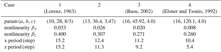
We next perform four numerical experiments by vary-ing the parameters (a,b,c): Case 1 uses the same pa-rameters as in Lorenz (1963) (Table 1); Case 2 multi-plies the parameters of Case 1 by the uniform factor of 1.3; Case 3 uses the parameters from Basu and Foufoula-Georgiou (2002); and Case 4, from Elsner and Tsonis (1992). The nature of the oscillations varies among the four cases (Fig. 5). For each case, 21 ensemble runs were made by adding one percent stochastic noise onto the initial data (i.e., the initial data xt o, yt o, zt o were changed to (1+0.01α1)xt o, (1+0.01α2)yt o, (1+0.01α3)zt o, where α1,

α2 andα3were Gaussian random numbers with zero mean

and unit standard deviation).

Table 1 listsβyandβzcalculated from Eq. (10) for the four cases. The main spectral periodsTxandTzdetermined from the power spectra ofx andz, respectively (Fig. 6) are also listed in Table 1. The spectral behavior ofy (not shown) is basically the same as as that forx, butzshows sharper spec-tral peaks thanx (Fig. 6). Proceeding inversely from Case 4 to Case 1, one finds a progressive increase inβyandβz, and inTxandTz, indicating that an increase in the nonlinearity of the system coincides with an increase in the spectral period of the oscillations.

Again (x,y,z) at timetwere used as predictors in nonlin-ear regression models to separately predict these three vari-ables at timet+lead time (where the lead time ranged from 0 to 20 time steps). Fig. 7 shows enhanced predictability (with higher correlation coefficient and lower MSE) forzas one proceeds inversely from Case 4 to Case 1, where the nonlin-earity of the system increased. This behavior in predictability was also found forx(not shown), though for a given level of correlation skill,xtends to have longer lead times thanz.

Since relative tox, the predictability lead time forztends to be shorter, and its main spectral periodTzis also≤Txand more sensitive to changes in the Lorenz system parameters (Table 1), we now focus onz. Its predictability lead time (for 0.80 correlation skill) divided by the main spectral periodTz is 0.69, 0.69, 0.70 and 0.65 for Cases 1 to 4, respectively, i.e. in all 4 cases, the nonlinear regression model when predict-ing ahead by 0.7 times the period inzcan attain a correla-tion skill of 0.8 for all four cases, thereby demonstrating that the enhanced predictability was basically due to the length-ened period of the oscillations when the nonlinearity of the Lorenz system was enhanced from Case 4 to Case 1. For the correlation skill of 0.95, its predictability lead time divided by the main spectral periodTz is 0.51, 0.50, 0.50 and 0.46 for Cases 1 to 4, respectively. So a similar conclusion can be drawn regardless of the correlation skill level chosen.

One potential problem with our calculation of βy and βz is that (0, 0, 0) has been used as the reference point, whereas the Lorenz attractor has two other equilibrium points (Drazin, 1992) which could also be chosen as the reference point (x0, y0, z0). If we replace (x, y, z) by

(x0+x0, y0+y0, z0+z0)in Eqs. (7)–(9), then drop the primes

for brevity, we get the Lorenz system with respect to the ref-erence point(x0, y0, z0):

dx/dt= −a(x+x0)+a(y+y0), (11)

dy/dt= −(x+x0)(z+z0)+b(x+x0)−(y+y0), (12)

0 10 20 30 40 50 60 0

5 10 15

x

Time

(a)

(b)

(c)

(d)

0 10 20 30 40 50 60

0 5 10 15

z

Time

(a)

(b)

(c)

(d)

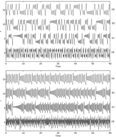
Figure 5: Normalized timeseries of x (top panel)and z (bottom panel)in the Lorenzmodel for (a) Case

1, (b)Case 2,() Case 3and (d)Case 4,where the time seriesfor dierent asesare vertially shiftedby

multiplesof5forlegibility.

20

0 10 20 30 40 50 60

0 5 10

x

Time

(b)

(c)

(d)

0 10 20 30 40 50 60

0 5 10 15

z

Time

(a)

(b)

(c)

(d)

Figure 5: Normalized time seriesof x (top panel)and z (bottom panel)in theLorenzmodel for(a) Case

1, (b)Case 2,() Case 3and (d) Case4,where the time series fordierent asesare vertially shiftedby

multiplesof5forlegibility.

20

Fig. 5. Normalized time series ofx(top panel) andz(bottom panel) in the Lorenz model for (a) Case 1, (b) Case 2, (c) Case 3 and (d)

Case 4, where the time series for different cases are vertically shifted by multiples of 5 for legibility.

The ratios of nonlinear to linear terms in Eqs. (12) and (13) are

βy=

h|xz|i

h|z₀x|+|x₀z|+|bx|+|y|i, βz=

h|xy|i

h|y₀x|+|x₀y|+|cz|i

. (14)

When the reference point is the equilibrium point (√c(b−1), √

c(b−1), b−1), the parameter βy is found to be 0.037, 0.027, 0.020, 0.008 for Cases 1 to 4, respectively; whileβz is 0.320, 0.296, 0.260, 0.245 for Cases 1 to 4. Similar re-sults are obtained if we choose the other equilibrium point

(−√c(b−1), −√c(b−1), b−1) as the reference. There-fore bothβyandβzdecrease as we proceed from Case 1 to Case 4, regardless of whether the origin or one of the other 2 equilibrium points has been chosen as the reference point.

0

2

4

0

Frequency

0

2

4

0

1

2

Spectrum

Frequency

(b)

x10

Figure 6: Ensemble mean power spetrum of the normalized (a) x and (b) z omponents. Dash, solid,

dash-dot anddottedlines representCase 1,2,3and 4,respetively.

0

2

4

0

Frequency

0

2

4

0

1

2

Spectrum

Frequency

(b)

x10

Figure 6: Ensemble mean power spetrum of the normalized (a) x and (b) z omponents. Dash, solid,

dash-dotand dottedlinesrepresentCase1,2,3and 4,respetively.

Fig. 6. Ensemble mean power spectrum of the normalized (a) x and (b) z components. Dash, solid, dash-dot and dotted lines represent

Case 1, 2, 3 and 4, respectively.

4 Summary and conclusion

Numerical coupled model results show that the predictability of ENSO is closely related to its nonlinearity and period. Un-der the post-1980s climatology, ENSOs have stronger non-linearity and longer period. The longer period enhances the system’s persistence, leading to better predictability. This behavior was also found in the Lorenz chaotic system, sug-gesting that it is not unusual for the increased nonlinearity of a climate system to enhance its predictability.

Lead time (x 0.05)

0 4 8 12 16 20

0 0.2 0.4 0.6 0.8

Lead time (x 0.05)

MSE

(a) (b) (c) (d)

Fig. 7. Ensemble mean predictability in terms of correlation skill

(top) and MSE (bottom) ofzin the Lorenz system, as given by the cross-validated correlation and MSE between the predicted and ac-tual time series. Dash, solid, dash-dot and dotted lines represent Case 1 (a), 2 (b), 3 (c) and 4 (d), respectively, with error bars show-ing±1 standard error.

Acknowledgements. This work was supported by the Natural

Sci-ences and Engineering Research Council of Canada via Discovery and Strategic grants to W. Hsieh.

Edited by: O. Talagrand

Reviewed by: four anonymous referees

References

An, S.-I. and Wang, B.: Interdecadal change of the structure of the ENSO mode and its impact on the ENSO frequency, J. Climate, 13, 2044–2055, 2000.

An, S.-I.: Interdecadal changes in the El Ni˜no La-Ni˜na asymmetry, Geophys. Res. Lett., 31, L23210, doi:10.1029/2004GL021699, 2004.

An, S.-I. and Jin, F.-F.: Nonlinearity and asymmetry of ENSO, J. Climate, 17, 2399–2412, 2004.

Basu, S. and Foufoula-Georgiou, E.: Detection of nonlinearity and chaoticity in time series using the transportation distance func-tion, Phys. Lett. A, 301, 413–423, 2002.

Bishop, C. M.: Neural Networks for Pattern Recognition, Claren-don Press, 482 pp., 1995.

Chen, D., Cane, M. A., Kaplan, A., Zebiak, S. E., and Huang, D.: Predictability of El Ni˜no in the past 148 years, Nature, 428, 733– 736, 2004.

Drazin, P. G.: Nonlinear Systems, Cambridge University Press, 317 pp., 1992.

Elsner, J. B. and Tsonis, A. A.: Nonlinear prediction, chaos and noise, B. Am. Meteorol. Soc., 73, 49–60, 1992.

Eccles, F. and Tziperman, E.: Nonlinear effects on ENSO’s period, J. Atmos. Sci., 61, 474–482, 2004.

Federov, A. V. and Philander, S. G.: A stability analysis of tropi-cal ocean-atmosphere interactions: Bridging measurements and theory for El Ni˜no, J. Clim., 14, 3086–3101, 2001.

Hsieh, W. W.: Nonlinear multivariate and time series analy-sis by neural network methods, Rev. Geophys., 42, RG1003, doi:10.1029/2002RG000112, 2004.

Ji, M., Leetmaa, A., and Kousky, V. E.: Coupled model predictions of ENSO during the 1980s and the 1990s at the National Centers for Environmental Prediction, J. Climate, 9, 3105–3120, 1996. Jin, F.-F., Neelin, D., and Ghil, M.: ENSO on the devil’s staircase,

Science, 264, 70–72, 1994.

Kirtman, B. P. and Schopf, P. S.: Decadal variability in ENSO pre-dictability and prediction, J. Climate, 11, 2804–2822, 1998. Kleeman, R. and Moore, A. M.: A theory for the limitation of

ENSO predictability due to stochastic atmospheric transients, J. Atmos. Sci., 54, 753–767, 1997.

Lorenz, E. N.: Deterministic non-periodic flow, J. Atmos. Sci., 20, 130–141, 1963.

M¨unnich, M., Cane, M. A., and Zebiak, S. E.: A study of self-excited oscillations of the tropical ocean-atmosphere system. Part II: Nonlinear cases, J. Atmos. Sci., 48, 1238–1248, 1991. Penland, C. and Sardeshmukh, P. D.:The optimal-growth of

tropi-cal sea-surface temperature anomalies, J. Climate, 8, 1999–2024, 1995.

Ye, Z. and Hsieh, W. W.: The influence of climate regime shift on ENSO, Clim. Dynam., 26, 823–833, doi:10.1007/s00382-005-0105-5, 2006.

Ye, Z. and Hsieh, W. W.: Changes in ENSO and associated over-turning circulations from enhanced greenhouse gases by the end of the 20th century, J. Climate, 21, 5745–5763, doi:10.1175-2008JCLI1580.1, 2008.

Zebiak, S. E. and Cane, M. A.: A model El Ni˜no-Southern Oscilla-tion, Mon. Weather Rev., 115, 2262–2278, 1987.