www.ocean-sci.net/13/61/2017/ doi:10.5194/os-13-61-2017
© Author(s) 2017. CC Attribution 3.0 License.
Numerical investigation of the Arctic ice–ocean boundary layer and
implications for air–sea gas fluxes
Arash Bigdeli1, Brice Loose1, An T. Nguyen2, and Sylvia T. Cole3
1Graduate School of Oceanography, University of Rhode Island, Rhode Island, 02882, USA
2Institute of Computational Engineering and Sciences, University of Texas at Austin, Austin, Texas, 78712, USA 3Woods Hole Oceanographic Institution, Woods Hole, Massachusetts, 02543, USA
Correspondence to:Arash Bigdeli (arash_bigdeli@uri.edu)
Received: 16 January 2016 – Published in Ocean Sci. Discuss.: 9 February 2016
Revised: 8 December 2016 – Accepted: 24 December 2016 – Published: 23 January 2017
Abstract. In ice-covered regions it is challenging to deter-mine constituent budgets – for heat and momentum, but also for biologically and climatically active gases like car-bon dioxide and methane. The harsh environment and rela-tive data scarcity make it difficult to characterize even the physical properties of the ocean surface. Here, we sought to evaluate if numerical model output helps us to better esti-mate the physical forcing that drives the air–sea gas exchange rate (k) in sea ice zones. We used the budget of radioactive 222Rn in the mixed layer to illustrate the effect that sea ice forcing has on gas budgets and air–sea gas exchange. Appro-priate constraint of the 222Rn budget requires estimates of sea ice velocity, concentration, mixed-layer depth, and wa-ter velocities, as well as their evolution in time and space along the Lagrangian drift track of a mixed-layer water par-cel. We used 36, 9 and 2 km horizontal resolution of re-gional Massachusetts Institute of Technology general circu-lation model (MITgcm) configuration with fine vertical spac-ing to evaluate the capability of the model to reproduce these parameters. We then compared the model results to exist-ing field data includexist-ing satellite, moorexist-ings and ice-tethered profilers. We found that mode sea ice coverage agrees with satellite-derived observation 88 to 98 % of the time when av-eraged over the Beaufort Gyre, and model sea ice speeds have 82 % correlation with observations. The model demon-strated the capacity to capture the broad trends in the mixed layer, although with a significant bias. Model water velocities showed only 29 % correlation with point-wise in situ data. This correlation remained low in all three model resolution simulations and we argued that is largely due to the quality of the input atmospheric forcing. Overall, we found that even
the coarse-resolution model can make a modest contribution to gas exchange parameterization, by resolving the time vari-ation of parameters that drive the 222Rn budget, including rate of mixed-layer change and sea ice forcings.
1 Introduction
The ocean surface is a dynamic region where momentum, heat and salt, as well as biogeochemical compounds, are ex-changed with the atmosphere and with the deep ocean. At the sea–air interface, gases of biogenic origin and geochemical significance are exchanged with the atmosphere. Theory in-dicates that the aqueous viscous sublayer, which has a length scale of 20 to 200 µm (Jähne and Haubecker, 1998), is the pri-mary bottleneck for air–water exchange. Limitations in mea-surement at this critical scale have led to approximations of sea–air gas exchange based on indirect measurements. Four approaches involving data are typically used (Bender et al., 2011): (1) parametrization of the turbulent kinetic energy (TKE) at the base of the viscous sublayer, (2) tracing pur-posefully injected gases (Ho et al., 2006; Nightingale et al., 2000), (3) micro-meteorological methods (Zemmelink et al., 2006, 2008; Blomquist et al., 2010; Salter et al., 2011), and (4) radon deficit method. Here, we examine the radon deficit method (4), together with a parameterization of the TKE forcing (1) that theoretically leads to the observed deficit in mixed-layer radon.
1999; Nightingale et al., 2000; Sweeney et al., 2007; Taka-hashi et al., 2009). In the polar oceans, wind energy and at-mospheric forcing are transferred in a more complex manner as a result of sea ice cover (Loose et al., 2009, 2014; Legge et al., 2015). Sea ice drift due to Ekman flow (McPhee and Martinson, 1992), freezing and melting of ice leads on the surface ocean (Morison et al., 1992) and short period waves (Wadhams et al., 1986; Kohout and Meylan, 2008) all con-stitute important sources of momentum transfer. Consider-ing the scarcity of data on marginally covered sea ice zones (Johnson et al., 2007; Gerdes and Köberle, 2007), especially during Arctic winter time, the environment is too poorly sam-pled to constrain these processes through direct measurement or empirical relationships.
Lacking sufficient data to constrain these processes, we wonder whether it is possible for a numerical model to ad-equately capture forcing of air–sea gas exchange in the sea ice zone and consequently improve predictions of air–sea flux. The parameters of interest are sea ice concentration (or fraction of open water), sea ice velocity, mixed-layer depth (MLD), and water current speed and direction in the ice– ocean boundary layer (IOBL) (Loose et al., 2014). Here we use the budget of222Rn gas in the IOBL as an example, be-cause the radon deficit method has emerged as one of the principle methods to estimate gas exchange velocity in ice-covered waters (Rutgers Van Der Loeff et al., 2014; Loose et al., 2016).
The radon deficit method involves sampling 222Rn and 226Ra in the mixed layer to examine any difference in the concentration or (radio) activity of the two species. Radon is a gas, radium is a cation; in the absence of gas ex-change 222Rn and226Ra enter secular equilibrium meaning the amount of222Rn produced is equal to decay rate of226Ra. Any missing 222Rn in the mixed layer is attributed to ex-change with atmosphere (Peng et al., 1979).
Since the222Rn concentration in air is very low (less than 5 %, Smethie et al., 1985) and considering that concentration is proportional to activity and/or decay rate A, we can use Eq. (1) to determine gas exchange. Wherekgas transfer ve-locity in (m d−1),AE is the activity or decay rate of 222Rn which in secular equilibrium is equal to 226Ra activity,AM is222Rn measured decay rate in the mixed layer,λis decay constant of222Rn (0.181 d−1)andhis the MLD.
k=AE/AM−1λh (1)
The MLD,h, is calculated from the measurements performed at the hydrographic stations during222Rn sampling process. Gas transfer velocities from Eq. (1) reflect the memory of 222Rn for a period of 2 to 4 weeks (Bender et al., 2011), which is 4 to 8 times the half-life of222Rn (3.8 days).
This memory integrates the physical oceanography prop-erties of the IOBL, including sea ice cover, MLD and water current speed. These processes are likely to vary significantly during this period and it is important to consider them as a source of uncertainty in Eq. (1). To illustrate this uncertainty,
Figure 1.A graphic illustration of two possible back trajectories for
a single sampling station.
consider a mixed layer that rapidly changes by a factor of 2 just prior to sampling for radon. If the mixed-layer becomes shallower by stratification,hwill be smaller by factor of 0.5 whileAE/ AM in the mixed layer remains the same. Based on Eq. (1), this causeskto be half of its true value. That is, prior to stratification, TKE forcing was sufficient to ventilate the ocean to a depth greater than the apparenth(Bender et al., 2011).
Conversely, if the mixed layer deepens due to mixing,h in-creases and a new parcel of water withAE/ AM=1 is added to the mixed layer, causing the activity ratio to come closer to unity. These two influences on Eq. (1) (increasingh and
AE/AMapproaching unity) work against each other, but the net effect is to causekto appear larger. The change of factor of 2 or higher (in case of convection) in MLD in less than two weeks has been observed during several studies (Acre-man and Jeffery, 2007; Ohno et al., 2008; Kara, 2003).
The “memory” of gas exchange forcing that radon experi-ences is further complicated by the presence of sea ice. Con-sider two alternate water parcel drift paths that lead to the 222Rn sampling station in the sea ice zone (Fig. 1). Path B demonstrates a history in which water column spends most its back trajectory under sea ice. Path “A” shows a water col-umn which experiences stratification and shoaling of MLD equal toδhwhen drifting through a region that is completely uncovered by ice. During most of Path “B” gas transfer hap-pens in form of diffusion through sea ice and it will have a very lowk(Crabeck et al., 2014; Loose et al., 2011), in con-trast Path “A” will have a greater radon deficit, but a smaller
hbecause of stratification. In either case, it is critical to take into account the time history of gas exchange forcing, includ-ing changes in the mixed-layer and ice cover, which has led to the apparent radon deficit at the time of measurement.
radon deficit. In other words, we require a Lagrangian back trajectory of water parcels to track the evolution of the mixed layer and its relative velocity 4 weeks prior to sampling.
Although satellite data, ice-tethered drifters (Krishfield et al., 2008) and moorings (Krishfield et al., 2014; Proshutinsky et al., 2009) have provided valuable seasonal and spatial in-formation about the sea ice zone, they do not track individual water parcels and tend to convolve space and time variations. The spatial limitation of these data poses a challenge to pro-ducing a back trajectory of the water parcel.
To address the above mentioned challenges, we use a suite of the Estimation of the Circulation and Climate of the Ocean (ECCO) project’s Arctic regional configurations to test the if a numerical model can be used to follow the back trajectory of a radon-labeled water parcel and the gas exchange forcing acting upon it and yield the missing information required for the Radon deficit method.
The variables and derived quantities of interest from the numerical model include MLD, sea ice concentration and speed (Loose et al., 2014), and the water velocity in the MLD. We note that as part of the Arctic Ocean Model Inter-comparison Project (AOMIP), a number of Arctic ocean-ice models’ capability to represent the main ice–ocean dynamics have been assessed (Proshutinsky et al., 2001; Lindsay and Rothrock, 1995, p. 995; Proshutinsky et al., 2008). Our rea-sons for choosing ECCO over other Arctic models stem from the higher correlation between the ECCO’s regional Arctic simulated outputs to satellite-derived sea ice data (Johnson et al., 2012) and the feasibility in the Massachusetts Institute of Technology general circulation model (MITgcm) to adapt a high near-surface vertical resolution to existing configura-tions.
The remainder of the article is organized as follows: in Sect. 2 we provide the details of the ECCO ice–ocean mod-els. Section 3.1 and 3.2 focus on model outputs of sea ice concentration and velocity and comparison with observations from satellite and ice-tethered profilers. Section 3.3 investi-gates the modeled output salinity and temperature structure and the resulting upper ocean density structure and mixed layer. Section 3.4 evaluates the correlation in near-surface water velocity. In Sect. 4 we discuss the results and sources of error and their impact on estimated gas exchange and lastly, Sect. 5 provides the summary of our results.
2 Method
2.1 ECCO model configurations
Three ECCO configurations are used, at horizontal grid spac-ings of 36, 9 and 2 km, respectively. The models are based on the MITgcm code and employ the z coordinate system described in Adcroft and Campin (2004). Our approach is to first assess the model outputs from the coarse-resolution model using model–data misfits, then to investigate if there
is quantitative reduction in model–data misfits with higher horizontal resolutions. Surface forcings are from the 25-year Japanese Reanalysis Project (JRA-25) (Onogi et al., 2007) for 36 and 9 km runs and the European Centre for Medium-Range Weather Forecasts (ECMWF) analysis for the 2 km run. Initial conditions are from World Ocean Atlas 2005 (Antonov et al., 2006; Locarnini et al., 2006) and initial sea ice conditions are from Zhang and Rothrock (2003) for 36 and 9 km, from which the models are allowed to spin up from 1992. The 2 km global run is initialized from a 4 km spin-up version of the ECCO adjoint-based state estimate for January 2011 and covers the period February 2011 to October 2012. The vertical mixing uses K profile parameterization (KPP) developed by Large et al. (1994) and 36 and 9 km runs utilize salt-plume parameterization (SPP) of Nguyen et al. (2009). The horizontal boundary condition for the 36 and 9 km con-figurations comes from existing global ECCO2 model out-puts (Marshall et al., 1997; Menemenlis et al., 2008; Losch et al., 2010; Heimbach et al., 2010).
We introduced a set of new vertical grid spacings to allow us to capture near-surface small details which cannot be rep-resented with the coarser grid system. In the 36 km (hereafter referred to as A1) and 9 km (called A2) models, the spacing is 2 m in the upper 50 m of the water column and gradually in-creases to a maximum of 650 m. In contrast, the 2 km model (called A3) has 25 layers in the top 100 m of water column, starting from 1 m and increasing to 15 m step. All the bound-ary conditions from ECCO2 have been interpolated to match the new vertical grid system.
2.2 Observations
Satellite-derived estimation of sea ice cover at 25 km hori-zontal resolution (Comiso, 2000) is interpolated to a horizon-tal grid system to facilitate model–data comparison. In addi-tion, sea ice drift gathered by 28 ice-tethered profilers (ITPs) (Krishfield et al., 2008) which have more than 2 months of data in the Beaufort Sea between 2006 and 2013 have been used to do the ice velocity comparison.
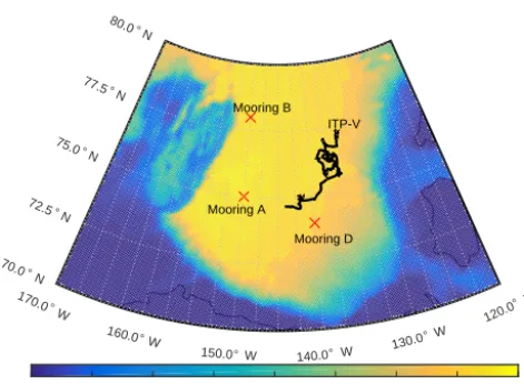
We compared near-surface water velocity data from an ice-tethered profiler with velocity instruments (ITP-V) (Williams et al., 2010) to A1 and A2 and an upward-looking acoustic doppler current profiler installed on a McLane moored pro-filer (MMP) (McPhee et al., 2009; Cole et al., 2014) to A1, A2 and A3 in order to compute the accuracy and feasibility of calculating back trajectory of parcels located in the mixed layer. We limit our comparison of ITP-V, which runs from October 2009 to March 2010, to A1 and A2 since those mod-els run from 2006 to 2013 and A3 runs from 2011 to 2013.
170.0
°
W 160.0
° W
150.0° W 140.0° W 130.0
° W 120.0
° W 70.0
°
N 72.5
° N
75.0
° N
77.5
° N
80.0
° N
ITP-V
Mooring A Mooring B
Mooring D
0 500 1000 1500 2000 2500 3000 3500 4000
Figure 2.Bathymetry and location of ITP-V and mooring for data
comparison.
depicts the bathymetry and location of most important obser-vations we used to make the comparisons with the model.
3 Results
3.1 Sea ice concentration
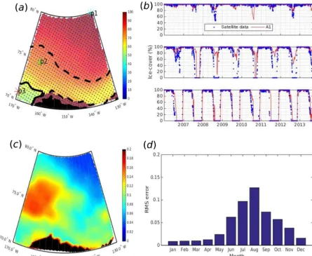
For sea ice concentration analysis we introduced a grid sys-tem covering the Beaufort Gyre and interpolated the data from satellite (Comiso, 2000) and A1 onto the grid. The anal-ysis grid extends from 70 to 80◦N and 130 to 170◦W, cov-ering most of Beaufort Gyre (Fig. 3). Grid points can be di-vided into two main geographic zones that are marked out based on sea ice cover. The first zone contains grid points where the annual average sea ice cover is greater than 80 %. These sets of points are fully covered by sea ice most of the year. The second zone can be described as “marginally ice covered” wherein the ocean surface is free of ice for some fraction of the year. We chose three points within this sea ice geography to compare the seasonal and interannual be-havior of the model with satellite ice cover. The points are located at 80◦N, 131.82◦W (P1), 70.82◦N, 169.82◦W (P2), and 74.76◦N, 163.51◦W (P3).
The ice cover at P1, P2 and P3 (Fig. 3) can be divided into 3 ice phases: (a) fully covered in ice, (b) open water and (c) a transition between (a) and (b). P3, which is the furthest south, has all three phases. In contrast P1 ice cover only dips below 60 % for two brief periods during the 7-year time series de-picted in Fig. 3 – once in 2008 and again in 2012. These three points illustrate where and when the model has the greatest challenge reproducing the actual sea ice cover. At the extrem-ities of the ice pack, where the water is predominantly cov-ered by 100 or 0 % ice (P1 and P3), the model captures the seasonal advance and retreat and the percentage of ice cover itself is accurate. However, in the transition regions that are characterized by marginal ice for much of the year (P2), the
model has more difficulty reproducing the observed sea ice cover as well as the timing of the advance and retreat. This behavior is consistent with the description that has been ex-plained by Johnson et al. (2007), that models have a higher accuracy predicting sea ice concentration in central Arctic and less accuracy near its periphery and the lower latitudes.
The spatial sensitivity of the model can be observed using root mean square (RMS) error (Hyndman and Koehler, 2006) Eq. (2), calculated over the 1992–2013 period (Fig. 3). The area with the highest misfits coincides with area between the 80 and 60 % contour lines (Fig. 3) and is concentrated pri-marily in the Western Beaufort. The RMSE error of 0.2 is the maximum value away from land, this same level of error can also be found near land which is caused by fast-ice gener-ation. Fast ice in the model is replaced with packs of drifting sea ice; this error is common among numerical models and has been brought to attention during AOMIP (Johnson et al., 2012).
RMSE(point)=
v u u t
n X
i=1
(Csimulation−Csatellite)2/n (2)
If we compare the monthly climatology for sea ice cover over the 1992–2013 period, the RMS error between model and satellite data is least during the early winter months (e.g., January–March) when sea ice is close to its maximum ex-tent. Comparing data and A1, Fig. 3 depicts an increase in RMSE during July, August, September and October and a minor decrease in May and November. The RMSE appears to be greater during the summer months of ice retreat, and slightly less during the autumn months of ice advance. Over-all, the periods of transition (melt and freeze) coincide with the greatest RMSE.
An important source of errors in the model ice concen-tration comes from the reanalysis surface forcing. Fenty and Heimbach (2012) showed that adjustments in the air temper-ature that are within the uncertainties of this reanalysis field can help bring the model ice edge into agreement with the observations. Of note also is that the uncertainty in satellite-derived ice cover can be the highest in the marginal ice zone due to tracking algorithms that are sensitive to cloud liquid water or cannot distinguish thin ice from open water (Ivanova et al., 2015); this error also manifests itself in quantification of model–data misfits.
3.2 Sea ice velocity
Figure 3. (a)Averaged satellite sea ice cover from 2006 to 2013, with the solid black line marking 60 % cover and dashed black line marking 80 %; blue dots show the analysis grid, stars show the location of the three points Cyan P1, Green P2 and Red P3 where time-series data is graphed in(b).(b)Time history of sea ice fraction from top P1, P2 and P3, with satellite data represented by blue dots, compared with A1.(c)Horizontal distribution of RMS error of A1 sea ice concentration averaged over time from 2006 to 2013; black mask covers the grid points on the land.(d)Spatially averaged annual RMS error of A1 sea ice concentration.
where ice is converging or diverging, these motions, relative to the motion of the water column, can produce significant changes in the water column momentum budget as well as air–sea fluxes. Thankfully, the ITPs can provide us with a measure of the real ice drift.
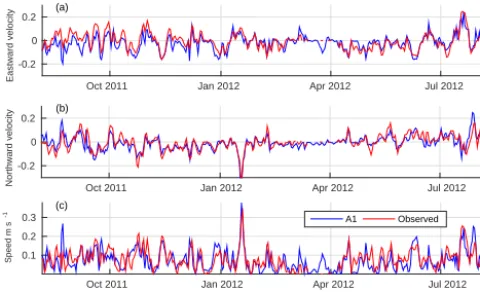
To generate a more quantitative comparison between the results, we utilized the same method introduced by Tim-mermans et al. (2011), to compare ice velocity components (eastward–northward) of A1 to ITP velocity and compute the correlation coefficient of each experiment with the daily-averaged actual drift velocity from the ITPs (Fig. 4).
When averaged over all the ITPs operating in Beaufort Gyre during 2006 to 2013, A1 had correlations of 0.8 with actual velocity components and 0.82 correlation with speed magnitude. RMSE calculated for A1 based on Eq. (2) shows an error of 0.043 ms−1and no significant bias.
3.3 Temperature, salinity, density and MLD 3.3.1 Vertical salinity and temperature profiles
We chose four hydrographic profiles in the Beaufort Sea to assess the simulated vertical salinity and temperature. The first two sets of profiles are from ITP-1 winter and summer 2006; the third set is from ITP-43 during winter 2010 and the fourth is from ITP-13 during summer 2008 (Fig. 5). For visualization we linearly extrapolated the profiles from the first layer of the model up to the surface, which occurs over the top 1 m of the water column.
Oct2011 Jan2012 Apr2012 Jul2012
Eastward velocity
-0.2 0 0.2
Oct2011 Jan2012 Apr2012 Jul2012
Northward velocity
-0.2 0 0.2
Date
Oct2011 Jan2012 Apr2012 Jul2012
Speed m
s
-1
0.1 0.2
0.3 A1 Observed
(a)
(b)
(c)
Figure 4.Time series of sea ice velocity components and speed of
ITP 53 vs. 36 km horizontal resolution of MITgcm (A1). The cor-relations between eastward, northward and magnitude of velocity between ITP 53 data and A1 are 78, 75 and 80 %, respectively.
however the ITP MLD is deeper by nearly 10 m, indicating more ice formation and convective heat loss over this water column, as compared to the model water column. In summer the model mixed-layer shoals to approximately 5 m depth following two local temperature extrema; the bigger maxi-mum is at∼35 m, generated by intrusion of the Pacific Sum-mer Water (PSW) which is a dominant feature in the Canada Basin. The second smaller maximum happens around 10 m called the summer mixed layer (Shimada et al., 2001, p. 201) or near-surface temperature maximum (NSTM) (Jackson et al., 2010) which is a seasonal feature generated by shortwave solar heat diffusion (Perovich and Maykut, 1990). These two well-defined phenomena are broadly descriptive of the sum-mer surface layer in the Beaufort Gyre. They are, however, absent from the ITP data at this location, indicating a differ-ent ice and heat budget time history.
Data and model profiles in Fig. 5b show better agreement in the shape and the absolute value of the T and S pro-files. Both model and ITP data have a 20 m deep mixed layer during 2010 winter. The model in this case does not show as much change in vertical temperature structure com-pared to actual data. In the profile from ITP-13 (Fig. 5) the model again over-estimates the temperature beneath the mixed layer, although certain features including the NSTM can still be found near 10 m, yet not as pronounced since it is very close to PSW. Bearing in mind that density in the Arc-tic is dominated by changes in salinity, we move forward to density profiles from this point on.
In addition, we note that recent studies show that eddies with diameters of 30 km or less (Nguyen et al., 2012; Spall et al., 2008; Zhao et al., 2014; Zhao and Timmermans, 2015; Zhao et al., 2016) play an important role in transporting Pa-cific water from the shelf break into the Canada Basin. Ad-equate representation of ocean eddies and investigation into their roles in setting the water column stratification require a model with finer horizontal resolution. Hence, moving
for-ward, in addition to A1, we utilize the 9 km model (A2) to investigate the density profiles as well as study the MLD.
3.3.2 Density profiles
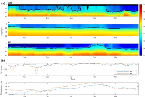
We compared the 36 and 9 km model outputs of density to the time series of density profiles from ITP-35 (Fig. 6) from October 2009 to March 2010. A black mask indicates loca-tions where there is no data from ITP-35 – particularly in the upper 7 m of the water column. As ITP-35 transited through the Canada Basin, density profiles contain both temporal and spatial changes.
We are able to discern some broad similarities between the model and ITP density profiles. From November through January, both ITP and model density profiles remain rela-tively constant. Between February and March, ITP-35 ap-pears to drift through a zone of convection, likely caused by ice formation, with a sudden increase of density near the sur-face. The same feature can be observed in both A1 and A2 density. However, on a smaller scale, there is significantly more variation in the ITP data than what the model repre-sents.
For exploring the reason behind the density signals, we used the simulated fraction of sea ice cover and ice thick-ness (Fig. 6). The dominating effect appears to result from a sea ice fraction when there is an almost continuously cov-ered area. The changes from sea ice thickness can be ob-served in the volume of fresh water in the water column, as seen by outcropping of the 1022.5 isopycnal coinciding with the increase of sea ice thickness. An increase in near-surface density can be seen in late January and early February ac-companied by an increase in ice thickness and insertion of brine in the water column. The second peak, which is not as pronounced, happens in late February when ice fraction de-creases from 100 to 95 % and exposes the surface water to cold atmosphere, leading to the production of newly formed sea ice. We further examine these signals in the MLD section below.
3.3.3 Mixed-layer depth
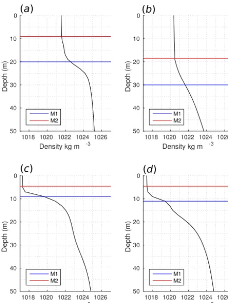
There are many different methods in the literature for cal-culating MLD (Brainerd and Gregg, 1995; Wijesekera and Gregg, 1996; Thomson and Fine, 2003; de Boyer Montégut et al., 2004; Lorbacher et al., 2006; Shaw et al., 2009). The methods can be divided into two main types (Dong et al., 2008): the first type of algorithm looks for the depth (zMLD) at which there has been a density increase ofδρ between the ocean surface andzMLD. A typical range of values for
δρare 0.005 to 0.125 kg m−3(Brainerd and Gregg, 1995; de Boyer Montégut et al., 2004). The second type uses slightly different criteria, where the base of the mixed layer is deter-mined as the depth where the gradient of density (∂ρ / ∂z) equals or exceeds a threshold; typical numbers for∂ρ / ∂z
Lor-Figure 5.Salinity and temperature of the top 70 m based on ITPs and A1.(a)ITP 1 on 13 December 2006 at 74.80◦N and 131.44◦W. (b)ITP-43 on 27 November 2010 at 75.41◦N and 143.09◦W.(c)ITP 1 on 28 August 2006 at 76.96◦N and 133.32◦W.(d)ITP-13 on 30 July 2008 at 75.00◦N and 132.78◦W.
bacher et al., 2006, p. 200). A more sophisticated approach to type 1 of these criteria is to utilize a differential between
ρ100 m−ρsurfaceas the cut of point (instead of using a fixed
δρ) to account for the effects of surfaceρ changes during winter and summer (Shaw et al., 2009). Here, we have im-plemented two of these methods M1 and M2, with M1 us-ing δρ equal to 0.2 ofρ100 m−ρsurface (Shaw et al., 2009) and M2 with a gradient (∂ρ / ∂z) cut off point equal to 0.02 kg m−4, which matches innate model parameterization of MLD (Nguyen et al., 2009).
We compare these two methods by applying them to the profiles from Fig. 5, and the results are shown in Fig. 7. In case (a) and (b) M1 produces a MLD that is 8 to 12 m deeper, compared to the other method. A visual examination of
pro-files indicates that the M1 criteria may be too flexible of a cri-teria. The results from M1 appear to be intermittently “realis-tic”, whereas M2 can be difficult to implement for data sam-pled at high vertical resolution as a result of greater small-scale variability. In practice, we find M1 is the most straight-forward to implement.
Figure 6. (a)Observed upper-ocean density vs. 36 km (A1) and 9 km (A2) resolution MITgcm density along the path of ITP drift; the black mask covers areas where no ITP data is available and solid black line shows isopycnal of 1022.5 kg m−3.(b)Simulated sea ice fraction and thickness on top of the water column.
profile whose MLD is less than 2 m below the shallowest ITP measurement is discarded. This restriction effectively re-moves any MLDs shallower than 10 m due to the ITP sampler not resolving the upper 8 m of water column. In some cases, a remnant mixed-layer from the previous winter may exist in the water column. In this case, the methods incorrectly iden-tify the remnant mixed layer (ML) as actual MLD.
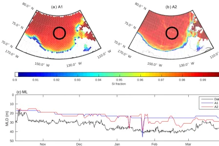
To compare the methods over a longer time period, we cal-culated the MLD from model data and ITP-35 data along the ITP-35 drift track. We used M1 to determine the MLD for A1, A2 and for ITP-35 data (Fig. 8). Both model results show a shallower ML compared to the ITP data; the most promi-nent feature in late January corresponds to a sudden change in density found in Fig. 6. Beside the above-mentioned peak, A1 fails to capture any variability in MLD whereas A2 shows that the ML deepens by about 10 m in mid February corre-sponding to ice opening occurring during the same time span (Fig. 6). The difference between A1 and A2, and their ability to capture MLD change, can be explained by the capability of a higher-resolution model to capture small-scale fractures in the ice cover (Fig. 8), and conversely, the inability of the coarser resolution to do so is due to averaging over a larger
de-Figure 7. Methods M1 and M2 applied to selected ITP profiles, (a)ITP 1 on 13 December 2006 at 74.80◦N, 131.44◦W.(b) ITP-43 on 27 November 2010 at 75.41◦N, 143.09◦W.(c)ITP 1 on 28 August 2006 at 76.96◦N, 133.32◦W.(d)ITP-13 on 30 July 2008 at 75.00◦N, 132.78◦W.
pendent on vertical grid spacing. We also investigated MLD in A3 (no SPP) run compared to A2, and confirmed that the average MLD is the same between these two runs.
3.4 Velocities in the water column
We have very little information from direct observations that permit us to track a water parcel, especially beneath sea ice. This is one area where model output could be critical as there are not obvious alternatives. To assess the consistency of the model water current field, we compared 2-D model water ve-locity to data gathered from two sources: (1) from ADCPs mounted on moorings that were deployed starting in 2008 in Beaufort Gyre (Proshutinsky et al., 2009) and (2) the ITP-V sensor equipped with MAVSs (Modular Acoustic Velocity Sensors) (Williams et al., 2010), which was the only operat-ing ITP before 2013 which had an acoustic sensor mounted on it.
We compared the velocity components averaged from 5 to 50 m to account for flow direction that is moving the water parcels in the mixed layer over the duration of ITP-V work-ing days, which was from 9 October 2009 to 31 March 2010
(Fig. 9). The ITP data has been daily averaged to remove higher frequency information which we do not expect the model to capture due to the low frequency (6-hourly) wind forcing. Both A1 and A2 show less than 0.3 correlations with data with no improvement in respect to resolution.
We further add A3 to our comparison for moorings veloc-ities (Fig. 9), and compared velocveloc-ities at 25 m, which is the level that is shared between all our models and removes the necessity of any interpolation. The simulation results show RMSE normalized by data of higher than 5 and correlations of less than 0.3 over three moorings and almost 2 years of data. This result indicates that ocean currents are not well captured in the model irrespective of horizontal grid reso-lution. We must therefore look into the atmospheric forcing as a likely source of error on high frequency water veloci-ties near the surface. As noted above, the wind inputs into the model from the reanalyses are available at a 6-hourly fre-quency. Chaudhuri et al. (2014) and Lindsay et al. (2014) have compared various available reanalysis products over the Arctic which we used to force our model, along with multi-ple other reanalysis products with available ship-based and weather station data, and found out that wind products in all of those have low correlation, i.e., less than 0.2. To investi-gate we compared JRA-55 (Onogi et al., 2007) and NCEP (Kalnay et al., 1996) to shipboard data gathered during 2014 in a time span of 2 months in the Arctic and found that JRA-55 had−0.20 correlation, RMSE of 7.36 and bias of−1.3, and NCEP had a correlation of 0.10, RMSE of 5.73 and bias of−1.40 when compared with high-frequency data on each cruise, reinforcing our suspicion of high-frequency wind as a source of error in water currents.
4 Gas exchange estimation
Up to this point we have spent extensive effort assessing the skill of the MITgcm to reproduce the key forcing parame-ters listed in our introduction. This effort is motivated by the potential for using the MITgcm model output as a tool to im-prove our ability to model gas budgets in the IOBL and to improve our estimates ofkin the sea ice zone, both of which depend on sea ice processes in the IOBL. To illustrate the po-tential impact that IOBL properties can have on the estimate ofk, we perform a simple experiment, using estimates ofk
over the range of variation in model output at three locations in the sea ice zone. The intention is to illustrate the variabil-ity inkand in the radon deficit that can arise as a result of sea ice processes.
4.1 Constraining gas exchange forcings
Utilizing the results from Sect. 3.1, 3.2 and 3.3, we calculated gas exchange velocities at P1, P2 and P3 (Fig. 10), over the course of the model simulation (i.e.,
170.0
° W
150.0° W
130.0° W
110.0
° W
70.0
° N
75.0
° N
80.0
° N (a ) A1
170.0
° W
150.0° W
130.0° W
110.0
° W
70.0
° N
75.0
° N
80.0
° N (b ) A2
SI fraction
0.9 0.91 0.92 0.93 0.94 0.95 0.96 0.97 0.98 0.99 1
Days
Nov Dec Jan Feb Mar
MLD (m)
0
10
20
30
40
50
(c) ML
Data A1 A2
Figure 8.Sea ice cover higher than 0.9 with gray circle marking the area of ITP operation for(a)36 km (A1) and(b)9 km(A2) horizontal
resolution of the model. A2 captured the ice opening and resulting mixed-layer change while this phenomenon has been averaged out by a (c)coarse-resolution model observed and simulated evolution of mixed-layer depth on the path of ITP.
gcm IOBL properties are fed to the estimator of k, consid-ering sea ice processes (Loose et al., 2014). Our selected points have the mean sea ice concentrations of 96.1, 87.62 and 61.69 %, sea ice speeds of 0.05, 0.086 and 0.10 ms−1, wind speeds of 8.73, 5.87 and 4.11 ms−1.
The result yields a point cloud of values that varies de-pending primarily on the range of ice velocity, wind speed and sea ice cover. The values of k range between 0.1 and 14.0, with a mean of 2.4 and standard deviation of 1.55. This exercise demonstrates the sensitivity ofkto the IOBL forc-ing parameters. In the event that we can trust the majority of the model outputs, such as the case here with high fidelity in the simulated SI concentration and SI velocities in A1, we conclude that a numerical model, even a coarse-resolution one, can make significant improvement to the estimate ofk. The question of constraining the radon budget within a La-grangian water parcel is somewhat more complicated.
4.2 Application of forcings on radon budget
The results in Sect. 3.4 showed that the difference between model and data water trajectories accumulated too much er-ror to be useful, and indicate that for a regional GCM to be useful for reconstructing the back trajectories of
radon-labeled water parcels, we will need improved wind-forcing fields. With current reanalysis products, finding the back tra-jectory of radon-labeled water parcels is not feasible. When improved wind fields are available, the Green’s functions ap-proach (Menemenlis et al., 2005; Nguyen et al., 2011) or adjoint method (Forget et al., 2015, p. 4; Wunsch and He-imbach, 2013) can be used to reduce misfits between mod-eled and observed MLD velocity and likely make the model a valuable tool for tracking back trajectories, either in a smaller domain or full Arctic regional configuration. A pos-sible source of wind data can be from shipboard measure-ments, assuming the measurements persist over 10 days in the given sampling station.
ac-Figure 9. (a)Daily-averaged velocity components from 5 to 50 m observed by ITP-V vs. those simulated by A1 and A2.(b) Daily-averaged velocity components at 25 m observed by mooring D vs. A1,A2 and A3.
counted for. Typically sea ice velocity is ∼5 times greater than vertically averaged water velocity in the mixed layer (Cole et al., 2014). In this regard, it may be acceptable to assume that the water parcel is stationary as long as ice ad-vection is accounted for. Hence, spatial averaging should ac-count for ice drift over the point of radon and radium sam-pling. The same logic also applies to the changes in the MLD and sea ice concentration. For example, gas exchange calcu-lated (Eq. 1) based on assumption of constant MLD of 27.5 m with limits of 5 to 50 m (Peralta-Ferriz and Woodgate 2015) would have limits of ±80 %, whereas gas exchange calcu-lated based on model MLD would have±50 % error and ac-counts for time variability. With the current level of uncer-tainty in reanalysis products and inherent heterogeneity of marginal sea ice zones, we suggest a mixed weighted com-bination of model outputs and shipboard data to be the way forward for constraining gas budget in sea ice zones.
5 Summary
We have used 36, 9 and 2 km versions of the ECCO ocean– sea ice coupled models based on the MITgcm to investigate whether numerical model outputs can be used to compensate for lack of data in constraining air–sea gas exchange rate in the Arctic. The goal is to understand if model outputs can improve estimation of gas exchange velocity calculation and to evaluate the capability of the model to fill in the missing information in the radon deficiency method. This systematic comparison of upper-ocean processes has revealed the fol-lowing.
The coarse-resolution model showed a good fidelity in re-gard to reproducing sea ice concentration. Depending on the
Figure 10.Gas exchange estimated model outputs of wind and sea
ice speed at locations P1: 77.4◦N, 143.6◦W, P2: 74.8◦N, 163.5◦W and P3: 70.59◦N, 159.4◦W from January 2006 to December 2012, Areas enclose the outputs around the mean and two standard devi-ation. The size of the points demonstrate the magnitude of the gas exchange velocities normalized by sea ice cover.
location and/or season, the error of simulated ice concen-tration varied between 0.02 and 0.2. Away from ice fronts or active melting/freezing zones the model tended to have higher accuracy. Even in the marginal ice zone, due to the potentially high error in the satellite-derived ice concentra-tion, the model can still be used to quantify the air–sea gas exchange rate, though with an expected higher uncertainty due to the combination of model and data errors. In addi-tion to sea ice concentraaddi-tion, we also found good correlaaddi-tion (82 %) between model ice speed and ITP drift.
The A1, A2 and A3 experiments consistently could not capture the water velocity observed in ITPs or mooring. We speculate that this discrepancy may be the result of the qual-ity of the reanalysis wind products that are forcing these models. The wind products have been shown to have poor correlation with observed data at high frequencies. Consid-ering that the response of near-surface water is occurs al-most simultaneously to the wind forcing, low correlation in wind velocity would have direct impact on the modeled near-surface water velocities and likely yield low correlations be-tween modeled and observed ocean currents. Conversely, the same wind fields at lower frequencies and on broader spatial scale have higher accuracy, as evidenced by the high correla-tion between the modeled and observed sea ice velocity.
Taking into accounts all the misfits through detailed model–data comparisons, we were able to quantify the use-fulness of a numerical model to improve gas exchange rate and parameterization methods. We showed an example of how the sea ice concentration, velocity and MLD can af-fect the gas exchange rate by up to 200 % in marginal sea ice zones and that the model outputs can help constrain this rate. By finding the low correlation in near-surface ocean ve-locities, irrespective of model horizontal resolution, we con-cluded that finding the back trajectory of radon-labeled water parcels is currently not feasible. Furthermore, we speculate as to the source for the common errors in our models, namely the high frequency and under-constrained atmospheric forc-ing fields, and identify alternative approaches to enable the use of a model to achieve the back trajectory calculation task. The alternative approach includes using the MITgcm Green’s functions and adjoint capability to help constrain the model ocean velocity to observations, and performing the simula-tions in a smaller dedicated domain based on the specific spatial distribution of data for both atmospheric winds and ocean currents in the mixed layer.
6 Data availability
Due to sheer volume of A0, A1 and A2 model outputs (89 GB per 3-D field), the simulation results are archived at NASA Supercomputing Center and NCAR GLADE stor-age system and can be extracted upon request by contacting the primary author. The observational data can be accessed through http://www.whoi.edu/page.do?pid=20781. The post-processing scripts utilized to compare the observational data and simulation results can be found in the Supplement.
The Supplement related to this article is available online at doi:10.5194/os-13-61-2017-supplement.
Acknowledgement. We gratefully acknowledge computational resources and support from the NASA Advanced Supercomputing (NAS) Division and from the JPL Supercomputing and Visual-ization Facility (SVF) and high-performance computing support from Yellowstone (ark:/85065/d7wd3xhc) provided by NCAR’s Computational and Information Systems Laboratory, sponsored by the National Science Foundation. The ice-tethered profiler data were collected and made available by the Ice-Tethered Profiler Program (Toole et al., 2011; Krishfield et al., 2008) based at the Woods Hole Oceanographic Institution (http://www.whoi.edu/itp). Funding for this research was provided by the NSF Arctic Natural Sciences program through Award # 1203558.
Edited by: D. Stevens
Reviewed by: two anonymous referees
References
Acreman, D. M. and Jeffery, C. D.: The Use of Argo for Validation and Tuning of Mixed Layer Models, Ocean Model., 19, 53–69, doi:10.1016/j.ocemod.2007.06.005, 2007.
Adcroft, A. and Campin, J.-M.: Rescaled Height Coordi-nates for Accurate Representation of Free-Surface Flows in Ocean Circulation Models, Ocean Model., 7, 269–284, doi:10.1016/j.ocemod.2003.09.003, 2004.
Antonov, J., Locarnini, R., Boyer, T., Mishonov, A., and Garcia, H.: World Ocean Atlas 2005 Vol. 2 Salinity, NOAA Atlas NESDIS, 62, NOAA, Silver Spring, Md, 2006.
Bender, M. L., Kinter, S., Cassar, N., and Wanninkhof, R.: Eval-uating Gas Transfer Velocity Parameterizations Using Upper Ocean Radon Distributions, J. Geophys. Res., 116, C02010, doi:10.1029/2009JC005805, 2011.
Blomquist, B. W., Huebert, B. J., Fairall, C. W., and Faloona, I. C.: Determining the sea-air flux of dimethylsulfide by eddy cor-relation using mass spectrometry, Atmos. Meas. Tech., 3, 1–20, doi:10.5194/amt-3-1-2010, 2010.
Brainerd, K. E. and Michael, C. G.: Surface Mixed and Mix-ing Layer Depths, Deep-Sea Res. Pt. I, 42, 1521–1543, doi:10.1016/0967-0637(95)00068-H, 1995.
Chaudhuri, A. H., Ponte, R. M., and Nguyen, A. T.: A Comparison of Atmospheric Reanalysis Products for the Arctic Ocean and Implications for Uncertainties in Air–Sea Fluxes, J. Climate, 27, 5411–1521, doi:10.1175/JCLI-D-13-00424.1, 2014.
Cole, S. T., Timmermans, M.-L., Toole, J. M., Krishfield, R. A., and Thwaites, F. T.: Ekman Veering, Internal Waves, and Turbulence Observed under Arctic Sea Ice, J. Phys. Oceanogr., 44, 1306– 1328, doi:10.1175/JPO-D-12-0191.1, 2014.
Comiso, J.: Bootstrap Sea Ice Concentrations from Nimbus-7 SMMR and DMSP SSM/I-SSMIS. Boulder, Colorado USA, NASA DAAC at the National Snow and Ice Data Center, 2000. Crabeck, O., Delille, B., Rysgaard, S., Thomas, D. N.,
Geil-fus, N.-X., Else, B., and Tison, J.-L.: First “in Situ” Deter-mination of Gas Transport Coefficients (DO2, DAr, and DN2)
from Bulk Gas Concentration Measurements (O2, N2, Ar) in
Natural Sea Ice, J. Geophys. Res.-Oceans, 119, 6655–6668, doi:10.1002/2014JC009849, 2014.
Ocean: An Examination of Profile Data and a Profile-Based Climatology, J. Geophys. Res.-Oceans, 109, C12003, doi:10.1029/2004JC002378, 2004.
Dong, S., Sprintall, J., Gille, S. T., and Talley, L.: Southern Ocean Mixed-Layer Depth from Argo Float Profiles, J. Geophys. Res.-Oceans, 113, C06013, doi:10.1029/2006JC004051, 2008. Fenty, I. and Heimbach, P.: Coupled Sea Ice–Ocean-State
Estima-tion in the Labrador Sea and Baffin Bay, J. Phys. Oceanogr., 43, 884–904, doi:10.1175/JPO-D-12-065.1, 2012.
Forget, G., Campin, J.-M., Heimbach, P., Hill, C. N., Ponte, R. M., and Wunsch, C.: ECCO version 4: an integrated framework for non-linear inverse modeling and global ocean state estimation, Geosci. Model Dev., 8, 3071–3104, doi:10.5194/gmd-8-3071-2015, 2015.
Gerdes, R. and KöBerle, C.: Comparison of Arctic Sea Ice Thick-ness Variability in IPCC Climate of the 20th Century Experi-ments and in Ocean-Sea Ice Hindcasts, J. Geophys. Res.-Oceans, 112, C04S13, doi:10.1029/2006JC003616, 2007.
Heimbach, P., Menemenlis, D., Losch, M., Campin, J.-M., and Hill, C.: On the Formulation of Sea-Ice Models. Part 2: Lessons from Multi-Year Adjoint Sea-Ice Export Sensitivities through the Canadian Arctic Archipelago, Ocean Model., 33, 145–158, doi:10.1016/j.ocemod.2010.02.002, 2010.
Ho, D. T., Law, C. S., Smitth, M. J., Schlosser, P., Harvey, M., and Hill, P.: Measurements of Air-Sea Gas Exchange at High Wind Speeds in the Southern Ocean: Implications for Global Parameterizations, Geophys. Res. Lett., 33, L16611, doi:10.1029/2006GL026817, 2006.
Hyndman, R. J. and Koehler, A. B.: Another Look at Mea-sures of Forecast Accuracy, Int. J. Forecasting, 22, 679–688, doi:10.1016/j.ijforecast.2006.03.001, 2006.
Ivanova, N., Pedersen, L. T., Tonboe, R. T., Kern, S., Heyg-ster, G., Lavergne, T., Sørensen, A., Saldo, R., Dybkjær, G., Brucker, L., and Shokr, M.: Inter-comparison and evaluation of sea ice algorithms: towards further identification of chal-lenges and optimal approach using passive microwave obser-vations, The Cryosphere, 9, 1797–1817, doi:10.5194/tc-9-1797-2015, 2015.
Jackson, J. M., Carmack, E. C., McLaughlin, F. A., Allen, S. E., and Ingram, R. G.: Identification, Characterization, and Change of the near-Surface Temperature Maximum in the Canada Basin, 1993–2008, J. Geophys. Res., 115, C05021, doi:10.1029/2009JC005265, 2010.
Jähne, B. and Haubecker, H.: Air-Water Gas Exchange, Annu. Rev. Fluid Mech., 30, 443–448, doi:10.1146/annurev.fluid.30.1.443, 1998.
Johnson, M., Gaffigan, S., Hunke, E., and Gerdes, R.: A Compar-ison of Arctic Ocean Sea Ice Concentration among the Coor-dinated AOMIP Model Experiments, J. Geophys. Res.-Oceans, 112, C04S11, doi:10.1029/2006JC003690, 2007.
Johnson, M., Proshutinsky, A., Aksenov, Y., Nguyen, A. T., Lind-say, R., Haas, C., Zhang, J., Diansky, N., Kwok, R., Maslowski, W., and Haekkinen, S.: Evaluation of Arctic Sea Ice Thickness Simulated by Arctic Ocean Model Intercomparison Project Mod-els, J. Geophys. Res., 117, C00D13, doi:10.1029/2011JC007257, 2012.
Kalnay, E., Kanamitsu, M., Kistler, R., Collins, W., Deaven, D., Gandin, L., Iredell, M., Saha, S., White, G., Woollen, J., and
Zhu, Y.: The NCEP/NCAR 40-year reanalysis project, B. Am. Meteorol. Soc., 77, 437–471, 1996.
Kara, A. B.: Mixed Layer Depth Variability over the Global Ocean, J. Geophys. Res., 108, 3079, doi:10.1029/2000JC000736, 2003. Kohout, A. L. and Meylan, M. H.: An Elastic Plate Model for Wave Attenuation and Ice Floe Breaking in the Marginal Ice Zone, J. Geophys. Res., 113, C09016, doi:10.1029/2007JC004434, 2008. Krishfield, R., Toole, J., Proshutinsky, A., and Timmermans, M.-L.: Automated Ice-Tethered Profilers for Seawater Observations under Pack Ice in All Seasons, J. Atmos. Ocean. Tech., 25, 2091– 2105, doi:10.1175/2008JTECHO587.1, 2008.
Krishfield, R. A., Proshutinsky, A., Tateyama, K., Williams, W. J., Carmack, E. C., McLaughlin, F. A., and Timmermans, M.-L.: Deterioration of Perennial Sea Ice in the Beaufort Gyre from 2003 to 2012 and Its Impact on the Oceanic Freshwater Cycle, J. Geophys. Res.-Oceans, 119, 1271–1305, doi:10.1002/2013JC008999, 2014.
Large, W. G., McWilliams, J. C., and Doney, S. C.: Oceanic Vertical Mixing: A Review and a Model with a Nonlocal Boundary Layer Parameterization, Rev. Geophys., 32, 363–403, doi:10.1029/94RG01872, 1994.
Legge, O. J., Bakker, D. C. E., Johnson, M. T., Meredith, M. P., Venables, H. J., Brown, P. J., and Lee, G. A.: The Sea-sonal Cycle of Ocean-Atmosphere CO2 Flux in Ryder Bay,
West Antarctic Peninsula, Geophys. Res. Lett., 42, 2934–2942, doi:10.1002/2015GL063796, 2015.
Lindsay, R., Wensnahan, M., Schweiger, A., and Zhang, J.: Evalua-tion of Seven Different Atmospheric Reanalysis Products in the Arctic, J. Climate, 27, 2588–2606, 2014.
Lindsay, R. W. and Rothrock, D. A.: Arctic Sea Ice Leads from Ad-vanced Very High Resolution Radiometer Images, J. Geophys. Res., 100, 4533–4544, 1995.
Locarnini, R., Mishonov, J., Boyer, T., Antonov, J. I., and Garcia, H. E.: World Ocean Atlas 2005, Vol. 1 Temreature, NOAA Atlas NESDIS 62 (NOAA, Silver Spring, Md.), 2006.
Loose, B., McGillis, W. R., Schlosser, P., Perovich, D., and Taka-hashi, T.: Effects of Freezing, Growth, and Ice Cover on Gas Transport Processes in Laboratory Seawater Experiments, Geo-phys. Res. Lett., 36, L05603, doi:10.1029/2008GL036318, 2009. Loose, B., Schlosser, P., Perovich, D., Ringelberg, D., Ho, D. T., Takahashi, T., Richter-Menge, J., Reynolds, C. M., Mcgillis, W. R., and Tison, J.-L.: Gas Diffusion through Columnar Labora-tory Sea Ice: Implications for Mixed-Layer Ventilation of CO2 in the Seasonal Ice Zone, Tellus B, 63, 23–39, doi:10.1111/j.1600-0889.2010.00506.x, 2011.
Loose, B., McGillis, W. R., Perovich, D., Zappa, C. J., and Schlosser, P.: A Parameter Model of Gas Exchange for the Sea-sonal Sea Ice Zone, Ocean Sci., 10, 1–16, doi:10.5194/os-10-1-2014, 2014.
Loose, B., Kelly, R., Bigdeli, A., Krishfield, R. A., Rutgers Van Der Loeff, M., and Moran, B.: How Well Does Wind Speed Predict Air-Sea Gas Transfer in the Sea Ice Zone? A Synthesis of Radon Deficit Profiles in the Upper Water Column of the Arctic Ocean, J. Geophys. Res., accepted, 2016.
Losch, M., Menemenlis, D., Campin, J.-M., Heimbach, P., and Hill, C.: On the Formulation of Sea-Ice Models. Part 1: Effects of Different Solver Implementations and Parameterizations, Ocean Model., 33, 129–144, doi:10.1016/j.ocemod.2009.12.008, 2010. Marshall, J., Adcroft, A., Hill, C., Perelman, L., and Heisey, C.: A Finite-Volume, Incompressible Navier Stokes Model for Studies of the Ocean on Parallel Computers, J. Geophys. Res.-Oceans, 102, 5753–5766, doi:10.1029/96JC02775, 1997.
McPhee, M. G.: Advances in Understanding Ice–ocean Stress dur-ing and since AIDJEX, Cold Reg. Sci. Technol., 76–77, 24–36, doi:10.1016/j.coldregions.2011.05.001, 2012.
McPhee, M. G., Proshutinsky, A., Morison, J. H., Steele, M., and Alkire, M. B.: Rapid Change in Freshwater Con-tent of the Arctic Ocean, Geophys. Res. Lett., 36, L04606, doi:10.1029/2008GL036587, 2009.
McPhee, M. and Martinson, D. G.: Turbulent Mixing under Drifting Pack Ice in the Weddell Sea, Science, 263, 218–220, 1992. Menemenlis, D., Fukumori, I., and Lee, T.: Using Green’s Functions
to Calibrate an Ocean General Circulation Model, Mon. Weather Rev., 133, 1224–1240, doi:10.1175/MWR2912.1, 2005. Menemenlis, D., Campin, J.-M., Heimbach, P., Hill, C., Lee, T.,
Nguyen, A., Schodlok, M., and Zhang, H.: ECCO2: High
Reso-lution Global Ocean and Sea Ice Data Synthesis, Mercator Ocean Quarterly Newsletter, 31, 13–21, 2008.
Morison, J. H., McPhee, M. G., Curtin, T. B., and Paulson, C. A.: The oceanography of winter leads, J. Geophys. Res., 97, 199–11, 1992.
Nguyen, A. T., Menemenlis, D., and Kwok, R.: Improved Mod-eling of the Arctic Halocline with a Subgrid-Scale Brine Rejection Parameterization, J. Geophys. Res., 114, C11014, doi:10.1029/2008JC005121, 2009.
Nguyen, A. T., Menemenlis, D., and Kwok, R.: Arctic Ice-Ocean Simulation with Optimized Model Parameters: Ap-proach and Assessment, J. Geophys. Res.-Oceans, 116, C04025, doi:10.1029/2010JC006573, 2011.
Nguyen, A. T., Kwok, R., and Menemenlis, D.: Source and Pathway of the Western Arctic Upper Halocline in a Data-Constrained Coupled Ocean and Sea Ice Model, J. Phys. Oceanogr., 42, 802– 823, doi:10.1175/JPO-D-11-040.1, 2012.
Nightingale, P. D., Malin, G. M., Law, C., Watson, A., Liss, P. S., Liddicoat, M. I., Boutin, J., and Upstill-Goddard, R. C.: In Situ Evaluation of Air-Sea Gas Exchange Parameterizations Using Novel Conservative and Volatile Tracers, Global Biogeochem. Cy., 14, 373–387, 2000.
Ohno, Y., Iwasaka, N., Kobashi, F., and Sato, Y.: Mixed Layer Depth Climatology of the North Pacific Based on Argo Observa-tions, J. Oceanogr., 65, 1–16, doi:10.1007/s10872-009-0001-4, 2008.
Onogi, K., Tsutsui, J., Koide, H., Sakamoto, M., Kobayashi, S., Hat-sushika, H., Matsumoto, T. et al.: The JRA-25 Reanalysis, J. Me-teorol. Soc. Jpn. Ser. II, 85, 369–432, doi:10.2151/jmsj.85.369, 2007.
Peng, T.-H., Broecker, W. S., Mathieu, G. G., and Li, Y.-H.: Radon Evasion Rates in the Atlantic and Pacific Oceans as Determined during the Geosecs Program, J. Geophys. Res., 84, 2471–2486, 1979.
Peralta-Ferriz, C. and Woodgate, R. A.: Seasonal and Interannual Variability of Pan-Arctic Surface Mixed Layer Properties from 1979 to 2012 from Hydrographic Data, and the Dominance
of Stratification for Multiyear Mixed Layer Depth Shoaling, Prog. Oceanogr., 134, 19–53, doi:10.1016/j.pocean.2014.12.005, 2015.
Perovich, D. and Maykut, G. A.: Solar Heating of a Stratified Ocean in the Presence of a Static Ice Cover, J. Geophys. Res., 95, 18233–18245, doi:10.1029/JC095iC10p18233, 1990.
Proshutinsky, A., Steele, M., Zhang, J., Holloway, G., Steiner, N., Hakkinen, S., Holland, D., Gerdes, R., Koeberle, C., Karcher, M., and Johnson, M.: Multinational Effort Studies Differences among Arctic Ocean Models, EOS Transact American Geophys-ical Union, 82, 637–644, doi:10.1029/01EO00365, 2001. Proshutinsky, A., Gerdes, R., Holland, D., Holloway, G. and
Steele, M.: AOMIP: Coordinated activities to improve mod-els and model predictions, CLIVAR Exchanges, 13 (1), (Ex-changes; 44), 17, http://eprints.soton.ac.uk/50120/01/Exch_44. pdf (last access: 20 September 2015), 2008.
Proshutinsky, A., Krishfield, R., Timmermans, M.-L., Toole, J., Car-mack, E., McLaughlin, F., Williams, W. J., Zimmermann, S., Itoh, M., and Shimada, K.: Beaufort Gyre Freshwater Reservoir: State and Variability from Observations, J. Geophys. Res., 114, C00A10, doi:10.1029/2008JC005104, 2009.
Rutgers Van Der Loeff, M., Cassar, N., Nicolaus, M., Rabe, B., and Stimac, I.: The Influence of Sea Ice Cover on Air-Sea Gas Exchange Estimated with Radon-222 Profiles, J. Geophys. Res.-Oceans, 119, 2735–2751, doi:10.1002/2013JC009321, 2014. Salter, M. E., Upstill-Goddard, R. C., Nightingale, P. D., Archer,
S. D., Blomquist, B., Ho, D. T., Huebert, B., Schlosser, P., and Yang, M.: Impact of an Artificial Surfactant Release on Air-Sea Gas Fluxes during Deep Ocean Gas Exchange Experiment II, J. Geophys. Res., 116, C11016, doi:10.1029/2011JC007023, 2011. Shaw, W. J., Stanton, T. P., McPhee, M. G., Morison, J. H., and Martinson, D. G.: Role of the Upper Ocean in the Energy Budget of Arctic Sea Ice during SHEBA, J. Geophys. Res., 114, C06012, doi:10.1029/2008JC004991, 2009.
Shimada, K., Carmack, E. C., Hatakeyama, K., and Takizawa, T.: Varieties of Shallow Temperature Maximum Waters in the West-ern Canadian Basin of the Arctic Ocean, Geophys. Res. Lett., 28, 3441–3444, 2001.
Smethie, W. M., Takahashi, T., Chipman, D. W., and Ledwell, J. R.: Gas Exchange and CO2Flux in the Tropical Atlantic Ocean
Determined from 222Rn andpCO2Measurements, J. Geophys.
Res.-Oceans, 90, 7005–7022, 1985.
Spall, M. A., Pickart, R. S., Fratantoni, P. S., and Plued-demann, A. J.: Western Arctic Shelfbreak Eddies: Forma-tion and Transport, J. Phys. Oceanogr., 38, 1644–1668, doi:10.1175/2007JPO3829.1, 2008.
Sweeney, C., Gloor, E., Jacobson, A. R., Key, R. M., McKin-ley, G., Sarmiento, J.-L., and Wanninkhof, R.: Constraining Global Air-Sea Gas Exchange for CO2 with Recent Bomb 14C Measurements, Global Biogeochem. Cy., 21, GB2015,
doi:10.1029/2006GB002784, 2007.
Takahashi, T., Sutherland, S. C., Wanninkhof, R., Sweeney, C., Feely, R. A., Chipman, D. W., Hales, B., Friederich, G., Chavez, F., Sabine, C., and Watson, A.: Climatological Mean and Decadal Change in Surface OceanpCO2, and Net Sea-Air CO2Flux over
the Global Oceans, Deep-Sea Res. Pt. II, 56, 554–577, 2009. Thomson, R. E. and Fine, I. V.: Estimating Mixed Layer Depth
doi:10.1175/1520-0426(2003)020<0319:EMLDFO>2.0.CO;2, 2003.
Timmermans, M.-L., Proshutinsky, A., Krishfield, R. A., Per-ovich, D. K., Richter-Menge, J. A., Stanton, T. P., and Toole, J. M.: Surface Freshening in the Arctic Ocean’s Eurasian Basin: An Apparent Consequence of Recent Change in the Wind-Driven Circulation, J. Geophys. Res., 116, C00D03, doi:10.1029/2011JC006975, 2011.
Toole, J. M., Timmermans, M. L., Perovich, D. K., Krishfield, R. A., Proshutinsky, A., and Richter-Menge, J. A.: Nfluences of the Ocean Surface Mixed Layer and Thermohaline Stratification on Arctic Sea Ice in the Central Canada Basin, J. Geophys. Res., 115, C10018, doi:10.1029/2009JC005660, 2010.
Wadhams, P., Squire, V. A., Ewing, J. A., and Pascal, R. W.: The Ef-fect of the Marginal Ice Zone on the Directional Wave Spectrum of the Ocean, J. Phys. Oceanogr., 16, 358–376, 1986.
Wanninkhof, R.: Relationship between Wind Speed and Gas Ex-change over the Ocean, J. Geophys. Res.-Oceans, 97, 7373– 7382, doi:10.1029/92JC00188, 1992.
Wanninkhof, R. and McGillis, W. R.: A Cubic Relationship between Air-Sea CO2Exchangeand Wind Speed, Geophys. Res. Lett., 26,
1889–1892, 1999.
Wijesekera, H. W. and Gregg, M. C.: Surface Layer Response to Weak Winds, Westerly Bursts, and Rain Squalls in the West-ern Pacific Warm Pool, J. Geophys. Res.-Oceans, 101, 977–997, doi:10.1029/95JC02553, 1996.
Williams, A. J., Thwaites, F. T., Morrison, A. T., Toole, J. M., and Krishfield, R. A.: Motion Tracking in an
Acoustic Point-Measurement Current Meter, IEEE,
doi:10.1109/OCEANSSYD.2010.5603862, 2010.
Wunsch, C. and Heimbach, P.: Dynamically and Kinematically Consistent Global Ocean Circulation and Ice State Estimates, in: In Ocean Circulation and Climate: A 21 Century Perspective, El-sevier, BV, https://dash.harvard.edu/handle/1/12136112 (last ac-cess: 14 January 2017), 2013.
Zemmelink, H. J., Delille, B., Tison, J. L., Hintsa, E. J., Houghton, L., and Dacey, J. W. H.: CO2Deposition over Multi-Year Ice
of the Western Weddell Sea, Geophys. Res. Lett., 33, L13606, doi:10.1029/2006GL026320, 2006.
Zemmelink, H. J., Dacey, J. W. H., Houghton, L., Hintsa, E. J., and Liss, P. S.: Dimethylsulfide Emissions over the Multi-Year Ice of the Western Weddell Sea, Geophys. Res. Lett., 35, L06603, doi:10.1029/2007GL031847, 2008.
Zhang, J. and Rothrock, D. A.: Modeling Global Sea Ice with a Thickness and Enthalpy Distribution Model in Generalized Curvilinear Coordinates, Mon. Weather Rev., 131, 845–861, doi:10.1175/1520-0493(2003)131<0845:MGSIWA>2.0.CO;2, 2003.
Zhao, M. and Timmermans, M.-L.: Vertical Scales and Dynamics of Eddies in the Arctic Ocean’s Canada Basin, J. Geophys. Res.-Oceans, 120, 8195–8209, doi:10.1002/2015JC011251, 2015. Zhao, M., Timmermans, M.-L., Cole, S., Krishfield, R.,
Proshutin-sky, A., and Toole, J.: Characterizing the Eddy Field in the Arc-tic Ocean Halocline, J. Geophys. Res.-Oceans, 119, 8800–8817, doi:10.1002/2014JC010488, 2014.