www.atmos-meas-tech.net/9/4915/2016/ doi:10.5194/amt-9-4915-2016
© Author(s) 2016. CC Attribution 3.0 License.
Quantifying the uncertainty of eddy covariance fluxes due to the use
of different software packages and combinations of processing steps
in two contrasting ecosystems
Ivan Mammarella, Olli Peltola, Annika Nordbo, Leena Järvi, and Üllar Rannik Department of Physics, University of Helsinki, P.O. Box 48, 00014 Helsinki, Finland
Correspondence to:Ivan Mammarella ([email protected])
Received: 23 October 2015 – Published in Atmos. Meas. Tech. Discuss.: 18 January 2016 Revised: 5 August 2016 – Accepted: 22 August 2016 – Published: 6 October 2016
Abstract.We have carried out an inter-comparison between EddyUH and EddyPro®, two public software packages for post-field processing of eddy covariance data. Datasets in-cluding carbon dioxide, methane and water vapour fluxes measured over 2 months at a wetland in southern Finland and carbon dioxide and water vapour fluxes measured over 3 months at an urban site in Helsinki were processed and analysed. The purpose was to estimate the flux uncertainty due to the use of different software packages and to evaluate the most critical processing steps, determining the largest de-viations in the calculated fluxes. Turbulent fluxes calculated with a reference combination of processing steps were in good agreement, the systematic difference between the two software packages being up to 2.0 and 6.7 % for half-hour and cumulative sum values, respectively. The raw data prepa-ration and processing steps were consistent between the soft-ware packages, and most of the deviations in the estimated fluxes were due to the flux corrections. Among the different calculation procedures analysed, the spectral correction had the biggest impact for closed-path latent heat fluxes, reach-ing a nocturnal median value of 15 % at the wetland site. We found up to a 43 % median value of deviation (with respect to the run with all corrections included) if the closed-path car-bon dioxide flux is calculated without the dilution correction, while the methane fluxes were up to 10 % lower without both dilution and spectroscopic corrections. The Webb–Pearman– Leuning (WPL) and spectroscopic corrections were the most critical steps for open-path systems. However, we found also large spectral correction factors for the open-path methane fluxes, due to the sensor separation effect.
1 Introduction
The eddy covariance (EC) technique is the most direct and defensible way to measure and calculate vertical turbulent fluxes of momentum, energy and gases between the atmo-sphere and bioatmo-sphere. During the last 3 decades, the num-ber of long-term EC stations all over the world has increased exponentially, covering a wide range of different ecosys-tem types (FLUXNET, www.fluxdata.org). EC is a technique analysing high-frequency wind and scalar atmospheric data series (often called “raw data”), usually saved in hard drive devices for post-field processing and final estimations of tur-bulent flux values. During the past years several attempts have been made to standardise the processing methodology, at least for carbon dioxide (CO2) and sensible and latent
heat (LE) fluxes (Aubinet et al., 2000, 2012; Lee et al., 2004). However, the harmonisation of data processing is quite dif-ficult, since most of the required steps and corrections are site-specific and instrument-specific (gas analyser and sonic anemometer). Nowadays, new and better instrumentation is available for measuring turbulent fluxes of energy and matter using the EC technique. Recent studies have compared com-mercially available gas analysers, focusing on precision, sta-bility and systematic and random errors both for CO2fluxes
(Burba et al., 2008; Ibrom et al., 2007a; Järvi et al., 2009) and methane (CH4)and nitrous oxide (N2O) fluxes (Detto et al.,
2011; Peltola et al., 2013, 2014; Rannik et al., 2015). How-ever, only a few studies have reported an inter-comparison between EC software packages, and all focusing only on en-ergy and CO2fluxes (Fratini and Mauder, 2014; Mauder et
sonic anemometer wind components and the different ap-proaches for high-frequency spectral correction are critical processing steps, giving differences up to 10 % in their study. Fratini and Mauder (2014) compared TK3 and EddyPro® software packages, achieving a satisfying agreement in cal-culated fluxes and related quality flags only after tuning the software processing steps and corrections to be similar. In fact, systematic differences in EC flux estimates strongly de-pend on the selection, application and order of processing steps, and the correct application, order and sometimes rele-vance and consequences of several processing steps are still topics under discussion (Aubinet et al., 2012; Mauder and Foken, 2006). In addition, the relevance of some process-ing steps and corrections depends not only on the system set-up, but also on meteorological conditions and ecosys-tem types (Mammarella et al., 2015; Nordbo et al., 2012). As a result, the EC processing software packages available to the community feature different implementations: some steps may be implemented using different methods (Mauder et al., 2007), while some operations and eventually further corrections suggested by recent findings are not supported by some of the software packages. This is particularly relevant for gases like CH4 and N2O, for which the deployment of
the EC system with easy-to-use fast response analysers have become popular only during the last decade. Therefore, nei-ther data processing approaches have yet been standardised nor software inter-comparison studies have been published for these gas fluxes.
In this study, we have performed an inter-comparison be-tween EddyUH and EddyPro, two public and commonly used software packages for EC data processing and calcula-tion. The aims are to estimate the flux uncertainty due to the use of different software packages for half-hour as well as for cumulative sums, and to assess the most critical process-ing steps, determinprocess-ing the largest deviations in the calculated fluxes. We focus not only on LE and CO2fluxes, as it has
been done in previous studies, but also on CH4fluxes.
2 Material and methods
2.1 Site description and measurements
The software inter-comparison was performed using datasets from two field sites in southern Finland. The first dataset was collected at the Siikaneva fen site (61◦49.9610N, 24◦11.5670E) during the CH
4 inter-comparison field
cam-paign (Peltola et al. 2013). The EC data used in this study were measured during 1 May–30 June 2010 with a 3-D sonic anemometer (USA-1, Metek GmbH), two closed-path gas analysers (LI-7000, LI-COR Biosciences; G1301-f, Picarro Inc.) and one open-path gas analyser (LI-7700, LI-COR Bio-sciences). LI-7700 was an early prototype version of the later commercialised LI-7700. LI-7000 measured CO2and water
vapour (H2O) and G1301-f measured CH4and H2O molar
fractions, whereas LI-7700 measured CH4molar
concentra-tions. LI-7000 and G1301-f used a shared heated sampling line that was approximately 16.8 m long (ID: 10 mm, flow rate: 24 L min−1). The sonic anemometer was situated 2.75 m above peat surface and the open-path LI-7700 directly below it, causing a 45 cm vertical separation between the sensors. Further details about the site and measurements can be found in Peltola et al. (2013).
The second dataset was collected between 1 July and 30 September 2010 at the Erottaja site located in Helsinki city centre (60◦09.9120N, 24◦56.7230E). The measurements rep-resent densely built-up urban area, with only 5 % of the sur-face being covered with vegetation. The measurements are carried out in a 3.8 m high mast located on top of a 38 m high fire station tower, resulting in a total height of 41.8 m. This is a sufficient height for the EC measurements as the mean building height in the surroundings of the tower is 21.7 m. The measurement set-up consisted of an ultrasonic anemometer (USA-1, Metek GmbH) to measure the wind components and open- and closed-path infrared gas analysers (LI-7500 and LI-7200, LI-COR Biosciences) for the CO2
and H2O fluctuations. Details of the measurement set-up can
be found in Nordbo et al. (2013). 2.2 Turbulent flux calculation
The turbulent fluxes of CO2(FCO2, µmol m
−2s−1)and CH 4
(FCH4, nmol m
−2s−1)and sensible (H, W m−2)and latent
(LE, W m−2)heat are calculated from the covariances be-tween a respective scalar and vertical wind velocity (w) as FCO2=
ρd
Ma
w0χ0
CO2, (1)
FCH4= ρd
Ma
w0χ0
CH4, (2)
H=ρdcpw0T0, (3)
LE=ρdLv
Mw
Ma
w0χ0
H2O, (4)
whereρdis the dry air density (kg m−3),cpthe specific heat
capacity of dry air (J kg−1K−1),Lvthe latent heat of
vapor-isation for water (J kg−1),Tthe temperature (K) andMaand Mwthe molar masses of dry air and water, respectively. The
termsw0T0,w0χ0 CO2,w
0χ0
CH4andw 0χ0
H2Oare the covariances
betweenwandT, dry mole fractions of CO2, CH4and H2O,
respectively. Overbars and primes represent temporal aver-aging and fluctuations, respectively.
2.3 Set-up of software runs
Covariance/EddyUHsoftware.php, and it was originally de-veloped in order to harmonise data processing among several EC sites operated by the group. Later, the software pack-age was made publicly available. The EddyUH processing flow chart (Fig. A1) is introduced in Appendix A, while a brief description of post-field data processing operations and methods, as presented in Table A1, is given in Appendices B and C.
The EddyUH software was compared against EddyPro, perhaps the most used software in the EC flux community, developed by LI-COR Biosciences Inc. (Lincoln, NE, USA). It is freely available and well documented (www.licor.com/ eddypro).
The eddy covariance datasets were processed using the reference combination of processing steps (Fig. 1) and avail-able methods implemented in EddyUH and EddyPro (Ta-ble 1). The applied methods were the same for most of the steps. However, some differences between software packages were present. In EddyUH the raw data despiking was done by the difference limit method (Appendix B), while in EddyPro the Vickers and Mahrt (1997) method was used. Different experimental methods were applied for spectral correction, e.g. according to Mammarella et al. (2009) in EddyUH and Fratini et al. (2012) in EddyPro. Moreover, additional correc-tion for water vapour cross-sensitivity (henceforth point-by-point spectroscopic correction) of closed-path CH4was done
in EddyUH according to Rella (2010). The same correction is not available in EddyPro. Finally, we performed four dif-ferent combinations of processing steps and compared them with the reference combination in order to evaluate the ef-fects of different calculation steps on the final flux estimates. The alternative runs were set up by modifying one step of the reference combination at a time. The first and second runs were done by excluding the spectral correction and ap-plying the theoretical approach (instead of experimental one used in the reference combination), respectively. The Webb– Pearman–Leuning (WPL) (Webb et al., 1980, henceforth also called dilution correction in the case of closed-path sensors) and spectroscopic corrections were omitted in the third run, and finally in the final run a constant value for the time lag was used.
Flux data were quality-screened prior to analysis. CH4flux
data were removed if the CH4mean mole fraction was above
5 or below 1.7 ppm. Additionally, LI-7700 fluxes were dis-carded if the received signal strength indicator (RSSI) was below 15. All the Siikaneva flux data were discarded if the second coordinate rotation angle (used to set w=0) was above 10◦. Wind direction (90–180◦ omitted) was used to
omit periods when the measurement system at the Erottaja site was in the wake of the building. In addition, periods when there were known problems with the measurement set-up at the Erottaja site were discarded. Plausibility limits were also used, since if the flux values were outside certain prede-fined limits they were thought to be erroneous. For Siikaneva data these limits were−50 and 160 nmol m−2s−1forFCH4,
−30 and 600 W m−2 for LE and−20 and 20 µmol m−2s−1 forFCO2. For Erottaja the following limits were used:−30
and 500 W m−2 for LE and −10 and 60 µmol m−2s−1 for
FCO2. Finally, flux data were discarded if the corresponding
quality flags, as determined by EddyUH and EddyPro, were above 5 based on the Foken et al. (2004) flagging policy. The data coverage obtained after data screening is given in Ta-ble 2.
3 Results
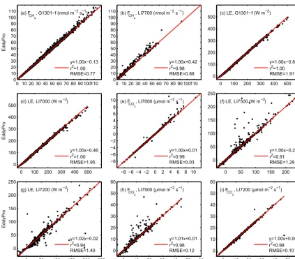
3.1 Flux comparison between software packages Fluxes measured by the same system were analysed and compared as estimated by the two software packages in the reference run. In terms of regression statistics, a very good agreement between EddyUH and EddyPro was ob-tained for LE andFCO2measured by LI-7000 (Fig. 2d and e),
LE and FCH4 by G1301-f at Siikaneva (Fig. 2c and a)
and FCO2 by LI-7200 at Erottaja (Fig. 2i). For LI-7500
LE and FCO2 no significant systematic differences
be-tween the software packages were found (Fig. 2f and h) even though the data show more scatter around the 1:1 line (r2=0.91, RMSE=1.29 W m−2for LE andr2=0.98, RMSE=0.12 µmol m−2s−1forFCO2)than the other
analy-sers. Instead, a systematic difference was found for LE mea-sured by the LI-7200 analyser in Erottaja, the EddyPro fluxes being 2 % higher than those calculated by EddyUH (Fig. 2g). Finally, good agreement resulted from the LI-7700 FCH4, the slope being equal to unity (r
2=0.98 and
RMSE=0.88 nmol m−2s−1; Fig. 2b). However, the
sen-sor separation correction in EddyPro (Horst and Lenschow, 2009) caused relatively large scatter between LI-7700 fluxes, and if the correction was omitted, visually the scatter be-tween the two software packages was reduced, although regression statistics were slightly worse (y=0.94x+0.51, RMSE=1.21 nmol m−2s−1,r2=0.99) (figure not shown). Applicability of the sensor separation correction for this par-ticular dataset is discussed in Sect. 4.2.
differ-Open-path analysers
Closed-path analysers
Iteration
Iteration
Relative magnitude of the processing routine
±2 %2
±25 % % *
1
3
-4...-7
< 1 % *4
± 1...5 % 1...5 % 5 6 4...12 % 5...35 % 5 6
1 2 3 4 5 6
Burba (2013), Moncrieff et al. (2004), Nordbo et al. (2012), This study, Peltola et al. (2013), Peltola et al. (2014),
7 8
Iwata et al. (2014), Järvi et al. (2009) * Comparison between methods
Despiking Coordinate rotation Time lag adjustment WPL correction Spectroscopic correction Spectral correction
Final flux Final flux Despiking Coordinate rotation Time lag adjustment Spectral correction
Processing at raw data level
Processing at covariance level
±2 %2
±25 % % *
1
3
-4...-7
<±1 % *4
NA
-1...-7 %4
±2 %2
±25 % % *
1
3
-4...-7
0...-7 % * 0...2 % 4 3 NA -8...-16 -12...-37 % %4 3
<±1%4* ±2 %2
±25 % % 1 3 * -4...-7 -1...-2 % 3 % 4 8 ±50 % -8...-38 % 1 4 NA <±1%4* ±2 %2
±25 % -4...-7 % 1 3 * -1...-3 % -4...-6 % 4 3 ±50 % -3...-15 % 1 4 NA
<±1%4* ±2 %2
±25 % % *
1
3
-4...-7
3...7 %5
-6...-10 %7
-30...105 % -4...21 % 5 7 -9...32 % 0...9 % 5 7
CH
4CO
2H O
2CH
4CO
2H O
2Relative magnitude of the processing routine Processing step Processing step
Calculation of z/L
Calculation of z/L
w’T ’s →w’T’ w’T ’s →w’T’
Dilution correction WPL correction Spectroscopic correction Spectroscopic correction 5...38 % 1...16 % 5 6
-3...43 %4
-1 %4
1...5 % 1...5 % 5 6 NA NA 5...38 % 1...16 % 5 6
-3...43 %4
-1 %4
Alternative route
Alternative route
F - F F
corr raw
raw
F - F |F |
corr raw
raw
F - F F
run ref
ref
1,8 5,6 2,3,4,7
Relative magnitude definition:
.
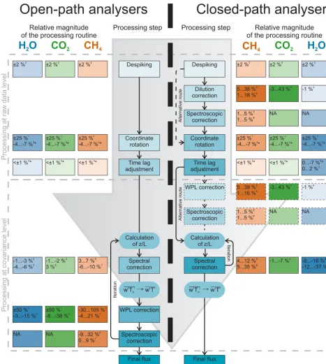
Figure 1.EC data processing scheme for open- and closed-path gas analyser data. Relative magnitude of each processing step is also reported, according to this and other studies. Note the different ways with different sign conventions (see footnotes) in which the relative magnitudes are calculated in different studies, whereFrawis the uncorrected flux,Frunthe flux without the corresponding correction,Fcorrthe flux after
the corresponding correction andFrefthe fully corrected flux. The reported percentages demonstrate the typical impact that the correction
0 10 20 30 40 50 60 70 80 90 100110 0 10 20 30 40 50 60 70 80 90 100 110 EddyPro
(a) FCH
4
, G1301−f (nmol m−2 s−1)
y=1.00x−0.13 r2=1.00 RMSE=0.77
0 10 20 30 40 50 60 70 80 90 100110 0 10 20 30 40 50 60 70 80 90 100 110 (b) F
CH4, LI7700 (nmol m −2 s−1)
y=1.00x+0.42 r2=0.98 RMSE=0.88
0 100 200 300 400 500
0 100 200 300 400
500 (c) LE, G1301−f (W m ) −2
y=1.00x−0.80 r2=1.00 RMSE=1.91
0 100 200 300 400 500
0 100 200 300 400 500 EddyPro
(d) LE, LI7000 (W m )−2
y=1.00x−0.46 r2=1.00 RMSE=1.95
−8 −6 −4 −2 0 2 4 6 8 10 −8 −6 −4 −2 0 2 4 6 8 10 (e) F
CO
2
, LI7000 (μmol m−2 s−1)
y=1.00x+0.01 r2=0.99 RMSE=0.03
0 50 100 150 200 250
0 50 100 150 200 250
(f) LE, LI7500 (W m )−2
y=1.00x−0.24 r2=0.91 RMSE=1.29
0 50 100 150 200 250
0 50 100 150 200 250 EddyUH EddyPro
(g) LE, LI7200 (W m )−2
y=1.02x−0.02 r2=0.94 RMSE=1.40
0 10 20 30 40 50 60
0 10 20 30 40 50 60 EddyUH (h) FCO
2
, LI7500 (μmol m−2 s−1)
y=1.01x+0.01 r2=0.98 RMSE=0.12
0 10 20 30 40 50 60
0 10 20 30 40 50 60 EddyUH (i) FCO
2
, LI7200 (μmol m−2 s−1)
y=1.00x+0.00 r2=0.99 RMSE=0.10
Figure 2.Comparison of the reference run fluxes estimated by EddyUH and EddyPro. CH4flux measured by G1301-f(a)and LI-7700(b),
LE measured by G1301-f(c)and LI-7000(d), CO2flux measured by LI-7000(e), LI-7500(h)and LI-7200(i)and LE measured by LI-7500
(f)and LI-7200(g). Each dot represents a 30 min data value. Dashed lines indicate the 1:1 line, and red solid lines the linear regression to
the data. Fluxes are measured at the Siikaneva fen site(a–e)and at the Erottaja urban site(f–i).
ence of 4 % (Fig. 3q). The reason was found to be a dif-ference in one of the inputs of the WPL temperature fluc-tuation term (T-term), specifically in the water vapour den-sity (ρw). In fact, while EddyUH uses the one from LI-7500,
EddyPro calculatesρwfrom meteorological relative
humid-ity (RH) data. For closed-path analysers or other open-path fluxes there is no difference in the WPL correction, and the uncorrected and WPL corrected curves follow similar pat-tern. The biggest differences between the software packages were related to the spectral corrections. For closed-path LI-7000 and G1301-f the fully corrected (e.g. WPL+SC in Fig. 3) LE fluxes were approximately 7 % larger at night-time in EddyUH than in EddyPro (Fig. 3m and k). How-ever, during these periods the absolute difference was still below 1 W m−2, since the night-time LE is small. This dif-ference is due to different RH dependence of low-pass filter time constant found between the two softwares (see
discus-sion in Sect. 4.1). For LI-7700FCH4 the relative difference
between the software packages was on average 12 % dur-ing the night, EddyPro fluxes bedur-ing larger (Fig. 3c), which corresponds to an absolute difference of 1–4 nmol m−2s−1
(Fig. 3d). This difference was related to the sensor separation correction, and the difference was smaller (4–10 % or 0.5– 1.5 nmol m−2s−1; EddyUH fluxes were larger) if the correc-tion was not done in EddyPro (see the corresponding discus-sion in Sect. 4.2).
3.2 Flux comparison between instruments
Fluxes measured with different gas analysers are com-pared as estimated using the reference combination in EddyUH and EddyPro (Fig. 4). At Erottaja, very good agreement was found between FCO2 measured by
0.8 1
EddyUH/EddyPro
−
a) FCH4, G1301−f a) FCH4, G1301−f (a) FCH4, G1301−f
0.8 1
−
c) FCH4, LI−7700 c) FCH4, LI−7700 (c) FCH4, LI−7700
−4 −2 0 2 nmol m −2 s −1
d) FCH4, LI−7700 d) FCH4, LI−7700 (d) FCH4, LI−7700
1 1.1 1.2
−
k) LE, G1301−f k) LE, G1301−f (k) LE, G1301−f
−1 0 1 2 3 W m −2
l) LE, G1301−f l) LE, G1301−f (l) LE, G1301−f
1 1.1 1.2
−
m) LE, LI−7000 m) LE, LI−7000 (m) LE, LI−7000
−1 0 1 2 3 W m −2
n) LE, LI−7000 n) LE, LI−7000 (n) LE, LI−7000 0.96 0.98 1 1.02 1.04 −
e) FCO2, LI−7000 e) FCO2, LI−7000 (e) FCO2, LI−7000
−0.1 0 0.1
μ
mol m
−2 s
−1
f) FCO2, LI−7000 f) FCO2, LI−7000 (f) FCO2, LI−7000
0.96 0.98 1 1.02 1.04 −
g) FCO2, LI−7200 g) FCO2, LI−7200 (g) FCO2, LI−7200
−0.1 0 0.1
μ
mol m
−2 s
−1
h) FCO2, LI−7200 h) FCO2, LI−7200 (h) FCO2, LI−7200
0.96 0.98 1 1.02 1.04 −
i) FCO2, LI−7500 i) FCO2, LI−7500 (i) FCO2, LI−7500
−0.1 0 0.1
μ
mol m
−2 s
−1
j) FCO2, LI−7500 j) FCO2, LI−7500 (j) FCO2, LI−7500
1 1.1 1.2
−
o) LE, LI−7200 o) LE, LI−7200 (o) LE, LI−7200
−1 0 1 2 3 W m −2
p) LE, LI−7200 p) LE, LI−7200 (p) LE, LI−7200
0 3 6 9 12 15 18 21
1 1.1 1.2
Time, UTC+2
−
q) LE, LI−7500 q) LE, LI−7500 (q) LE, LI−7500
0 3 6 9 12 15 18 21
−1 0 1 2 3 Time, UTC+2 W m −2
r) LE, LI−7500 r) LE, LI−7500 (r) LE, LI−7500
−4 −2 0 2 EddyUH − EddyPro
nmol m
−2 s
−1
b) FCH4, G1301−f b) FCH4, G1301−f (b) FCH4, G1301−f
Uncorrected WPL WPL+SC
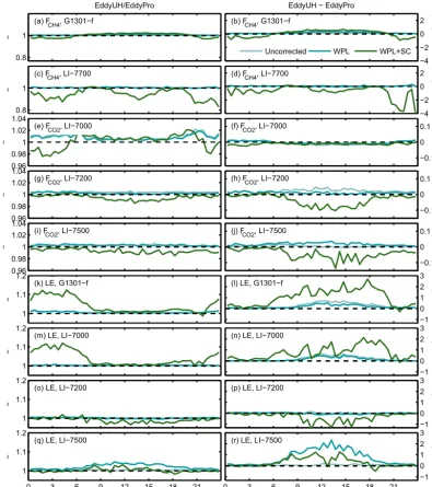
Figure 3.Median diurnal variation of flux ratio (left side) and bias (right side) for the studied instruments and variables between the two software. Light blue shows the uncorrected fluxes after despiking, coordinate rotation, detrending and time lag compensation; blue the WPL
corrected fluxes (for G1301-f and LI-7700FCH4 this includes also spectroscopic correction); and green the WPL plus spectral corrections
(WPL+SC). The WPL+SC curves represent data from the reference run, i.e. data that are fully corrected.
were obtained by using EddyUH (slope=0.99, r2=0.92, RMSE=1.25 µmol m−2s−1) and EddyPro (slope=0.98, r2=0.90, RMSE=1.32 µmol m−2s−1). LE measured by the same gas analysers show slightly weaker correspon-dence, the slope and RMSE being 1.02 and 8.15 W m−2 for EddyUH and 1.06 and 8.36 W m−2 for the EddyPro run, respectively (Fig. 4g and h). The small difference in LE between the two software packages is likely due to the spectral corrections (see below). Overall, the results are in agreement with Nordbo et al. (2013), who also found a better agreement between FCO2 than LE measurements at
the same site. A very good correspondence (slope=0.97, r2=1.00, RMSE=1.94 W m−2) was found between LE measured by LI-7000 and G1301 systems for the EddyUH reference run at the Siikaneva site (Fig. 4c). For EddyPro similar statistics were obtained (slope=0.96, r2=1.00, RMSE=2.56 W m−2 in Fig. 4d). By using the reference combination in the EddyUH run, a relative good agreement was also obtained betweenFCH4 values measured by G1301
be-0 10 20 30 40 50 60 70 80 0 10 20 30 40 50 60 70 80
FCH4, G1301−f (nmol m−2s−1) FCH4
, LI−7700 (nmol m
−2s −1)
EddyUH
(a) Siikaneva wetland
y=1.09x−1.19 r2=0.84 RMSE=2.64
0 10 20 30 40 50 60 70 80 0
10 20 30 40 50 60 70 80
FCH4, G1301−f (nmol m−2s−1)
FCH4
, LI−7700 (nmol m
−2s −1)
EddyPro
(b) Siikaneva wetland
y=1.16x−1.09 r2=0.86 RMSE=3.05
0 100 200 300 400 500
0 100 200 300 400 500
LE, G1301−f (W m−2)
LE, LI−7000 (W m
−2)
(c) Siikaneva wetland
y=0.97x+0.30 r2=1.00 RMSE=1.94
0 100 200 300 400 500
0 100 200 300 400 500
LE, G1301−f (W m−2)
LE, LI−7000 (W m
−2)
(d) Siikaneva wetland
y=0.96x+0.68 r2=1.00 RMSE=2.56
0 10 20 30 40 50 60
0 10 20 30 40 50 60
FCO2, LI−7500 (μmol m−2s−1) FCO2
, LI−7200 (
μ
mol m
−2s −1)
(e) Erottaja urban site
y=0.99x+0.49 r2=0.92 RMSE=1.25
0 10 20 30 40 50 60
0 10 20 30 40 50 60
FCO2, LI−7500 (μmol m−2s−1)
FCO2
, LI−7200 (
μ
mol m
−2s −1)
(f) Erottaja urban site
y=0.98x+0.50 r2=0.90 RMSE=1.32
0 50 100 150 200 250
0 50 100 150 200 250
LE, LI−7500 (W m−2)
LE, LI−7200 (W m
−2)
(g) Erottaja urban site
y=1.02x−0.35 r2=0.95 RMSE=8.15
0 50 100 150 200 250
0 50 100 150 200 250
LE, LI−7500 (W m−2)
LE, LI−7200 (W m
−2)
(h) Erottaja urban site
y=1.06x−0.65 r2=0.90 RMSE=8.36
Figure 4.Scatter plots ofFCH4 measured by G1301-f and LI-7700(a, b), LE measured by G1301-f and LI-7000(c, d),FCO2 measured
by LI-7500 and LI-7200(e, f)and LE measured by LI-7500 and LI-7200(g, h). Subplots in the left column show fluxes calculated with
EddyUH, and those in the right column fluxes calculated with EddyPro. Each dot represents a 30 min data value. Dashed lines indicate the 1:1 line, and red solid lines the linear regression to the data.
tween the two FCH4 values was found in the EddyPro run
(Fig. 4b), because of larger spectral correction estimates for the open-path gas analyser (see Sect. 4.2).
3.3 Effects of different flux processing combinations The impact of calculation steps on the final flux estimates in EddyUH and EddyPro is presented as deviation (in %) from the reference run for Siikaneva (Fig. 5) and Erottaja (Fig. 6) datasets. For closed-path systems in Siikaneva, the run with-out spectral correction had the largest effect on LE, being (in the EddyUH run) 14 and 9 % lower for G1301-f, and 16 and 12 % lower for the LI-7000 system, during night-time and daytime, respectively (Fig. 5c and d). When compared to
the EddyUH run, slightly smaller deviations (10 and 8 % for G1301-f and 12 and 11 % for the LI-7000) were found in the EddyPro run, but the trend in the deviations was consistent between the software packages. A similar range of deviations was found in Erottaja LE measured by LI-7200 (Fig. 6b). However, performing the theoretical spectral correction on the Siikaneva LE had a minimal effect (Fig. 5c and d), while the deviations found in LE measured by LI-7200 at Erottaja ranged between 6 and 3 % (Fig. 6b). The use of a constant time lag produces a small effect on LE, except during night-time when the higher RH increases the sorption of H2O in the
sampling line walls (Nordbo et al., 2014), and H2O time lag
No spec Theor spec No WPL Const lag −40
−20 0 20 40
(Run−ref)/ref (%)
(a) FCH4, G1301−f
No spec Theor spec No WPL Const lag −80 −60 −40 −20 0 20 40 60
(Run−ref)/ref (%)
(b) FCH4, LI−7700
No spec Theor spec No WPL Const lag −40
−20 0 20 40
(Run−ref)/ref (%)
(c) LE, G1301−f
No spec Theor spec No WPL Const lag −40 −20 0 20 40
(Run−ref)/ref (%)
(d) LE, LI−7000
No spec Theor spec No WPL Const lag −80
−60 −40 −200 20 40 60
(Run−ref)/ref (%)
(e) FCO2 LI−7000 EddyUH night
EddyPro night EddyUH day EddyPro day
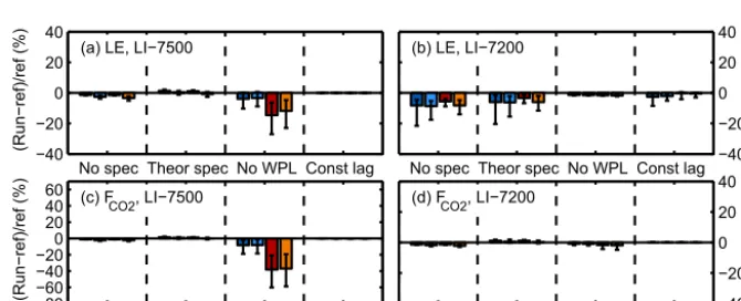
Figure 5.Effect of different calculation procedure of the estimated flux at the Siikaneva site, presented as deviation (in %) from the reference run (ref). Deviation is defined as (run-ref)/ref, where run refers to the run performed with no spectral correction (no spec), theoretical spectral correction (theor spec), no WPL (or dilution) and spectroscopic correction (no WPL) and using a constant time lag (const lag). Bars indicate
the median values, and error bars denote 25th and 75th percentiles. Note the different scale onyaxis in the subplots(b, e)compared to
(a, c, d).
No spec Theor spec No WPL Const lag −40
−20 0 20 40
(Run−ref)/ref (%)
(a) LE, LI−7500
No spec Theor spec No WPL Const lag −40 −20 0 20 40
(Run−ref)/ref (%)
(b) LE, LI−7200
No spec Theor spec No WPL Const lag −80
−60 −40 −200 20 40 60
(Run−ref)/ref (%)
(c) FCO2, LI−7500
No spec Theor spec No WPL Const lag −40 −20 0 20 40
(Run−ref)/ref (%)
(d) FCO2, LI−7200
Figure 6.As in Fig. 5, but for Erottaja. Note the different scale onyaxis in the subplots(c)compared to(a, b, d).
and FCH4 measured by LI-7000 and G1301-f systems,
re-spectively, with respect to the experimental spectral correc-tion (used in the reference run). If the LI-7000FCO2 is
cal-culated without performing the dilution correction (e.g. us-ing the wet mole fraction), we obtained 43 % higher day-time CO2 uptake with both software packages, and about
3 % lower positive fluxes during night-time. The same cor-rection also has a relevant impact on daytimeFCH4 measured
by G1301-f, resulting in 10 and 6 % deviations in EddyUH and EddyPro, respectively.
For open-path systems the critical step is represented by the WPL (and spectroscopic) correction. In Erottaja, the net CO2 emission calculated from LI-7500 data without WPL
correction is underestimated by 38 and 37 % during daytime in EddyUH and EddyPro, respectively (Fig. 6c). Instead, the nocturnal FCO2 is 8 % smaller than from the reference run.
Although the effect of no WPL is lower on LE, the calcu-lated deviations are still relevant, being 15 and 12 % dur-ing daytime (in EddyUH and EddyPro, respectively), and 4 and 3 % during night-time. Finally, in Siikaneva the LI-7700 FCH4calculated in EddyUH without the combined WPL and
spectroscopic correction shows −71 and 20 % deviations from the reference run during daytime and night-time. The same median values estimated in EddyPro are−67 and 18 % (Fig. 5b). In addition, it can be seen from the same figure that the deviation of nocturnalFCH4calculated without
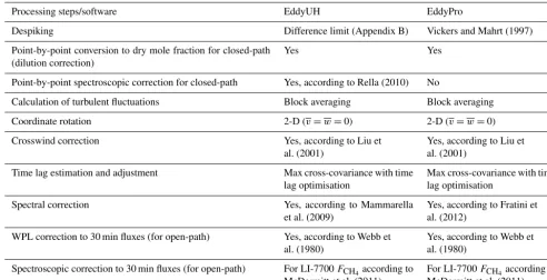
Table 1.Software set-ups for the reference combination.
Processing steps/software EddyUH EddyPro
Despiking Difference limit (Appendix B) Vickers and Mahrt (1997)
Point-by-point conversion to dry mole fraction for closed-path (dilution correction)
Yes Yes
Point-by-point spectroscopic correction for closed-path Yes, according to Rella (2010) No
Calculation of turbulent fluctuations Block averaging Block averaging
Coordinate rotation 2-D (v=w=0) 2-D (v=w=0)
Crosswind correction Yes, according to Liu et
al. (2001)
Yes, according to Liu et al. (2001)
Time lag estimation and adjustment Max cross-covariance with time
lag optimisation
Max cross-covariance with time lag optimisation
Spectral correction Yes, according to Mammarella
et al. (2009)
Yes, according to Fratini et al. (2012)
WPL correction to 30 min fluxes (for open-path) Yes, according to Webb et
al. (1980)
Yes, according to Webb et al. (1980)
Spectroscopic correction to 30 min fluxes (for open-path) For LI-7700FCH4according to
McDermitt et al. (2011)
For LI-7700FCH4according to
McDermitt et al. (2011)
3.4 Differences between cumulative fluxes
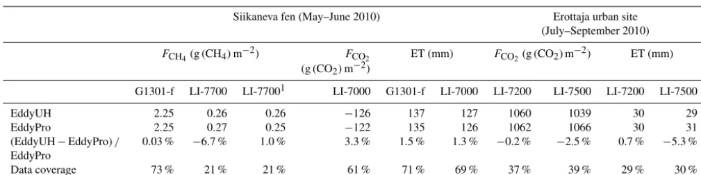
Cumulative sums of non-gap-filled flux time series are mostly within ±2 %, which suggests that there is no sig-nificant systematic bias between the two software packages (Table 2). Biggest relative differences were in LI-7700FCH4
and LI-7500 H2O flux cumulative sums,−6.7 and−5.3 %,
respectively, meaning that the cumulative values estimated with EddyPro were somewhat larger than with EddyUH. For LI-7700FCH4, if the sensor separation correction was
omit-ted, the relative difference was 1.0 % (EddyUH fluxes larger). The smallest relative difference was obtained for G1301-f cu-mulativeFCH4, 0.03 %.
The absolute differences between the cumulative CH4
fluxes at Siikaneva fen during the period May–June 2010 were−0.02 g (CH4)m−2(LI-7700, EddyPro larger) and less
than 0.01 g (CH4)m−2 (G1301-f) (Table 2). The difference
between cumulative CO2 fluxes was −4 g (CO2)m−2;
Ed-dyUH was showing slightly higher CO2uptake. This
orig-inated from the fact that EddyPro estimated approximately 1–3 % higher respiration at night and EddyUH calculated < 1 % higher uptake during daytime (cf. Fig. 3e). These dif-ferences were caused by the spectral corrections and they inflicted the observed deviation between the cumulative LI-7000 CO2 fluxes. At the Erottaja urban site during July–
September 2010 EddyUH showed slightly lower cumulative CO2 emission (−2 g (CO2)m−2) for LI-7200, whereas for
LI-7500 the difference was larger (−27 g (CO2)m−2).
Sim-ilarly, as in the case of LI-7000 CO2fluxes, here the
differ-ence observed between LI-7500 cumulative FCO2 was also
likely caused by the spectral corrections (cf. Fig. 3i). The cu-mulative H2O fluxes were within 2 mm. However, the data
coverage should be considered when evaluating the signifi-cance of these absolute differences. The data coverage of the Siikaneva measurements was between 73 % (CH4, G1301-f)
and 21 % (CH4, LI-7700). At the Erottaja site lower data
cov-erage was obtained (between 37 % (CO2, LI-7500) and 29 %
(H2O, LI-7500 and LI-7200)).
4 Discussion
0.2 0.3 0.4 0.5 0.6 0.7 0.8 0.9 0
0.2 0.4 0.6 0.8 1
Response time (s)
Siikaneva, Picarro G1301−f
(a) H2O, EddyUH, estimated
H2O, EddyUH, fitted CH4, EddyUH, estimated H2O, EddyPro, estimated H2O, EddyPro, fitted CH4, EddyPro, estimated
0.2 0.3 0.4 0.5 0.6 0.7 0.8 0.9 0 0.2 0.4 0.6 0.8 1
RH/100 (−)
Response time (s)
Siikaneva, LI−COR LI−7000
(b) H2O, EddyUH, estimated
H2O, EddyUH, fitted CO2, EddyUH, estimated H2O, EddyPro, estimated H2O, EddyPro, fitted CO2, EddyPro, estimated
0.2 0.3 0.4 0.5 0.6 0.7 0.8 0.9 0
0.5 1 1.5 2 2.5 3
RH/100 (−)
Response time (s)
Erottaja, LI−COR LI−7200
(c) H2O, EddyUH, estimated
H2O, EddyUH, fitted CO2, EddyUH, estimated H2O, EddyPro, estimated H2O, EddyPro, fitted CO2, EddyPro, estimated
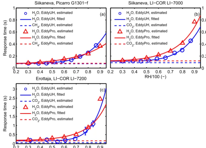
Figure 7.Relative humidity (RH) dependence of low-pass filter time constant as estimated with the two software packages. Note the different scale onyaxis in the subplot(c).
4.1 Critical steps and recommendations for closed-path systems
EC measurements from three closed-path systems (LI-7000, LI-7200 and G1301-f) were processed, and the impact of dif-ferent processing step combinations was analysed using runs performed with EddyUH and EddyPro. Among the different calculation procedures analysed, the spectral correction was the most relevant for the closed-path LE measurements at the two sites, the median values being between 6 and 16 %. On average, the use of theoretical spectral correction gave up to 6 % lower LE in Erottaja, while in Siikaneva the devi-ation respect to the reference run was generally below 3 %. We determined a stronger RH dependence of low-pass filter time constant in Erottaja than in Siikaneva (Fig. 7) caused by the non-heated sampling line there (Nordbo et al., 2013). Moreover, because of different approaches in the spectral correction methods, the low-pass filter time constants mated by EddyPro in Erottaja were larger than those esti-mated by EddyUH for RH values lower than 80 % (Fig. 7c). This may explain the 2 % difference between LI-7200 LE as estimated by EddyPro and EddyUH (Fig. 2g). Although the relative magnitudes of spectral corrections are not di-rectly comparable with other studies, they are in the same range as previously reported (Fig. 1). Surprisingly, at Si-ikaneva the theoretical spectral correction gave on average 7 % higher FCO2 and FCH4 than the experimental spectral
correction, and the result was consistent between the soft-ware packages. A possible explanation could be that in the
site-specific co-spectral model used in the reference run, the co-spectral peak frequencynm=0.056 estimated in unsta-ble conditions is shifted to lower frequencies respect to the Kaimal et al. (1972)-based atmospheric surface layer (ASL) co-spectral model used in the theoretical spectral correction (Moncrieff et al., 1997). In addition, in stable conditions the stability dependence of the estimatednmis less pronounced, and it does not follow the ASL parameterisation strictly (data not shown). This would result in smaller spectral corrections when using the site-specific co-spectral model in Eq. (C2). Generally it is thought that the theoretical approach easily underestimates the high-frequency spectral attenuation for closed-path systems, because of potential variations in the mass flow rates and relative uncertainty in the flow regime (Aubinet et al., 2000). Recent studies, both in the lab and in the field, have also demonstrated the important effects that different dust filters and rain caps (typically mounted at the tube inlet) have on the EC system cut-off frequency (Aubinet et al., 2016; Metzger et al., 2016). Such effects are not in-cluded in the theoretical approach. However, we have shown in this study how the use of a site-specific co-spectral model can reverse the relative magnitude of spectral correction cal-culated with the experimental approach compared to the one obtained via the theoretical approach.
In addition, we found that in Siikaneva the LI-7000FCO2
was greatly affected by the dilution effect due to large H2O
Table 2. Cumulative sums estimated with EddyUH and EddyPro. Relative differences and data coverage are also shown. Data were not gap-filled prior to calculation of the cumulative sums.
Siikaneva fen (May–June 2010) Erottaja urban site (July–September 2010)
FCH4(g (CH4)m
−2) F
CO2 ET (mm) FCO2(g (CO2) m
−2) ET (mm)
(g (CO2)m−2)
G1301-f LI-7700 LI-77001 LI-7000 G1301-f LI-7000 LI-7200 LI-7500 LI-7200 LI-7500 EddyUH 2.25 0.26 0.26 −126 137 127 1060 1039 30 29 EddyPro 2.25 0.27 0.25 −122 135 126 1062 1066 30 31 (EddyUH−EddyPro)/ 0.03 % −6.7 % 1.0 % 3.3 % 1.5 % 1.3 % −0.2 % −2.5 % 0.7 % −5.3 % EddyPro
Data coverage 73 % 21 % 21 % 61 % 71 % 69 % 37 % 39 % 29 % 30 %
1No sensor separation correction in EddyPro.
measured by G1301-f, because the flux to concentration ra-tio for CH4was larger than the one for CO2. In Erottaja the
same effect onFCO2 measured by LI-7200 was much lower
(on average 2 %), because of the 3 times smaller daytime val-ues of LE at this urban site. Besides this, the sampling line was not heated in Erottaja, and different magnitude of the dilution correction between the two sites was expected. In fact, although the heating (and insulation) of the sampling line decreased the H2O low-pass filter effect (especially at
increasing values of RH), at the same time it increased the H2O fluctuations in the sampled air, leading to larger
dilu-tion correcdilu-tion. It is common to think that the WPL and spec-troscopic corrections have small importance for closed-path analysers, since the temperature fluctuations are dampened in the sampling tube (Leuning and Judd, 1996; Rannik et al., 1997). However, this depends on the magnitude of H2O
fluc-tuations, which, as we have demonstrated here, is related to the ecosystem type and system set-up. Fortunately, current closed-path gas analysers also report H2O turbulent signals,
and the measured gas mole fractions can be readily converted into dry mole fractions, either in the analyser internal soft-ware or in the post-field data processing by using the point-by-point dilution and spectroscopic corrections.
Finally, for our sites and datasets, the use of nominal con-stant time lag was only an issue for nocturnal LE, when the absorption effect on H2O in the sampling line became more
relevant, determining an increase of H2O time lag, and thus
flux underestimations of 2 and 7 % in Siikaneva and 3 % in Erottaja, respectively (see Figs. 5c and d, 6b). Daytime de-viations were very small because of the strategy adopted for searching the H2O time lag (see Appendix B).
4.2 Critical steps and recommendations for open-path systems
For open-path gas analysers the WPL correction is the most critical step, and although it depends on ecosystem type, sea-son and target gas, the WPL correction terms can often sur-pass the magnitude of the flux itself and also change the sign
of the measured target gas flux (e.g. Peltola et al., 2013). Thus it is critical to perform this correction accurately, es-pecially when small target gas fluxes co-occur with largeH and LE fluxes. Here, we have shown that LI-7500FCO2
val-ues, measured at Erottaja urban site, are underestimated by 38 % on average if the correction is omitted, and the im-pact of the combined WPL and spectroscopic correction is even larger for LI-7700FCH4 measured at the Siikaneva fen
site (Sect. 3.3). A 2 % difference of daytime values ofH, as calculated by the two software packages, was found in Si-ikaneva (data not shown). The difference stems from the fact that in EddyUH a site-specific co-spectral model is used in the spectral correction, whereas EddyPro uses the co-spectral model from Moncrieff et al. (1997) in doing the spectral cor-rection toH. Nevertheless, the effect on WPL and spectro-scopic correction terms for LI-7700FCH4 was negligible, as
seen in Fig. 3.
If the response time which characterises the measurement system ability to measure the flux contribution of small ed-dies, i.e. high frequencies, is determined using power spec-tra, as done in EddyPro (Fratini et al., 2012), then the high-frequency dampening caused by spatial sensor separation needs to be estimated separately. In EddyPro it was done using the method proposed by Horst and Lenschow (2009), while EddyUH uses cospectra to estimate the measurement system’s high-frequency response, and thus no additional correction for sensor separation is needed. The Horst and Lenschow (2009) method is based on co-spectral peak fre-quency (nm)parameterisations against the stability parame-terζ, in addition to the ASL co-spectral model (as presented in Horst, 1997). Using these assumptions, they derived a de-pendence between the signal dampening due to sensor sepa-ration and the co-spectral peak wavenumber and sensor sep-aration in crosswind, along-wind and vertical directions.
For LI-7700 at the Siikaneva site, it was shown that this correction resulted in systematic differences between the software packages (Sect. 3.4) and between the two co-located CH4instruments (Sect. 3.2). The correction method seemed
fluxes that are too high. As mentioned above, the correction method relies onnmvs.ζparameterisations and Horst (1997) co-spectral model and, if these do not comply with the spec-tral characteristics of turbulence observed at the site, then the correction will be biased. Furthermore, LI-7700 was situ-ated significantly below the sonic anemometer (0.45 m) when compared with the sonic measurement height (2.75 m), and possibly, in such cases, the correction method does not per-form well. Nevertheless, the difference observed in this study emphasises the need for accurate spectral corrections and the importance of minimising the sensor separation when constructing an EC measurement set-up. The sensor separa-tion correcsepara-tions are especially important for open-path anal-ysers, since they cannot be mounted very close to the sonic anemometer due to their size and the flow distortion they may create.
5 Conclusions
We have estimated and analysed the flux uncertainty due to the use of two software packages, using datasets 2 and 3 months long including CO2, CH4 and LE fluxes measured
over a wetland and an urban site in Finland. Outputs from Ed-dyUH and EddyPro, two popular software packages for post-field processing of eddy covariance data, were compared. We evaluated the most critical processing steps, determining the largest deviations in the calculated fluxes. We found that the raw data preparation and processing steps were consistent be-tween the software packages, and most of the deviations in the estimated fluxes were due to the flux corrections. Among
the different calculation procedures analysed, the spectral correction was the most relevant for closed-path LE fluxes, reaching a night-time median value of 15 % at the wetland site. We found up to 43 % deviation (with respect the ref-erence run) if the closed-path CO2flux is calculated
with-out the dilution correction, while the CH4fluxes were up to
10 % lower without dilution and spectroscopic corrections. The WPL (and spectroscopic) correction was the most criti-cal step for open-path systems. However, we also found large spectral correction factors for the open-path CH4fluxes, due
to the sensor separation effect. Turbulent fluxes calculated with a reference combination of processing steps were in good agreement, the systematic difference between the two software packages being up to 2 and 6.7 % for half-hour and 2-month cumulative sum values, respectively. This re-sult is an improvement with respect to earlier software inter-comparison studies (e.g. Mauder et al., 2008), and it suggests that a consistent choice of implemented methods for the post-field processing steps can minimise the systematic flux un-certainty due to the usage of different software packages. Fi-nally, it is recommended for future studies that the impacts of processing steps on fluxes are investigated in more detail, including validation of new methods and corrections across different types of compounds/instruments and ecosystems.
6 Data availability
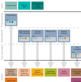
Appendix A: General description of EddyUH
EddyUH (https://www.atm.helsinki.fi/Eddy_Covariance/ EddyUHsoftware.php) is written in MATLAB and includes a graphical user interface (GUI). In order to advance methodological issues (concerning especially CH4and N2O
fluxes), besides standardised procedures, the most recent corrections and methods have also been implemented in EddyUH (see Table A1).
Post-field EC data processing with EddyUH is done through user-defined projects. A project in this context means a certain time period of data from a certain site that are pro-cessed with certain user-defined processing methods. These methods are determined by the user using the GUI and are saved in a set-up file where the site specifics and measure-ment system characteristics among other things are also de-fined. Therefore, all the processed data are always related to the saved project. The same project may include up to five different gas analysers combined with the same ultra-sonic anemometer, giving the possibility for the user to process several raw datasets at the same time. The software includes
Project set-up Raw EC data
Turbulence statistics, time lags, quality statistics
Spectra and Cospectra
Response times, H O response time vs. RH
2
Lag time statistics, H O lag vs. RH2
Coordinate
rotation planes cospectraModel Final outputdataset Flux calculation
Input: Spectral
analysis
Input: Planar fit tool
Input: Time lag optimiser
Input: High-frequency TRF estimation
Input: Preprocessor
Input:
Input
Preprocessing
Subprograms
Flux calculation
Output
Meteorological data (T, P, RH)
Footprints
Figure A1.Flow chart of EddyUH.
a number of modules, which operate at different levels of post-processing (Fig. A1). Preliminary fluxes are calculated in the preprocessor, where the first level of processing is done to the raw dataset. Then several corrections are ap-plied in the flux-calculation module, and the final fluxes are calculated (Table A1). In order to optimise the processing and properly apply all needed corrections, several software tools are available (Fig. A1). Co-spectral data are used in the high-frequency spectral transfer function estimator, where the low-pass filter time constant is experimentally estimated for each gas according to Mammarella et al. (2009). This ap-proach is particularly relevant in the case of closed-path sys-tems. Further, the time lag optimiser is a useful tool to verify the correctness of the chosen time lag window (and eventu-ally refine it) for each gas, as well as to determine the varying window boundaries for H2O as explained in Appendix B.
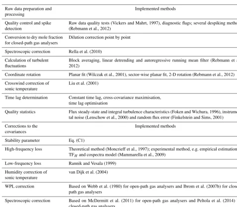
Table A1.List of implemented methods for data processing in EddyUH.
Raw data preparation and processing
Implemented methods
Quality control and spike detection
Raw data quality tests (Vickers and Mahrt, 1997), diagnostic flags; several despiking methods (Rebmann et al., 2012)
Conversion to dry mole fraction for closed-path gas analysers
Dilution correction point by point
Spectroscopic correction Rella et al. (2010)
Calculation of turbulent fluctuations
Block averaging, linear detrending and autoregressive running mean filter (Rebmann et al., 2012)
Coordinate rotation Planar fit (Wilczak et al., 2001), sector-wise planar fit, 2-D rotation (Rebmann et al., 2012)
Crosswind correction of sonic temperature
Liu et al. (2001)
Time lag determination Constant time lag, cross-covariance maximisation,
time lag optimisation
Quality statistics Flux steady-state and integral turbulence characteristics (Foken and Wichura, 1996),
instrumen-tal noise (Lenschow et al., 2000) and random flux error (Finkelstein and Sims, 2001)
Corrections to the covariances
Implemented methods
Stability parameter Eq. (C1)
High-frequency loss Theoretical method (Moncrieff et al., 1997); experimental method, e.g. empirical estimation of
TFH and cospectra model (Mammarella et al., 2009)
Low-frequency loss Rannik and Vesala (1999)
Humidity correction of sonic temperature
van Dijk et al. (2004)
WPL correction Based on Webb et al. (1980) for open-path gas analysers and Ibrom et al. (2007b) for
closed-path gas analysers
Spectroscopic correction Based on McDermitt et al. (2011) for open-path gas analysers and Peltola et al. (2014) for
Appendix B: Raw data preparation and processing in EddyUH
In the first level of data processing several operations are done to the raw dataset in order to calculate uncorrected co-variances of interest. Several methods related to these pro-cessing steps are available (see Table A1), and they are briefly presented below.
B1 Quality control and despiking
The raw data are quality-flagged according to physical plau-sible ranges of high-frequency values of each variable, diag-nostic parameters (if available) and several tests, as described in Vickers and Mahrt (1997). Further spikes are then de-tected, and commonly, this is done applying the Vickers and Mahrt (1997) method. However, other methods also exist in EddyUH, e.g. the difference limits method, which compare the difference between consecutive data points to a given threshold for each raw data time series (see Rebmann et al., 2012 for more details). If the time series contains too many spikes, the data might be useless and a flux should not be calculated for the averaging period of interest (commonly 30 min). Foken (2008) suggests excluding time series with more than 1 % spikes from further analysis.
B2 Point-by-point conversion to dry mole fraction for closed-path gas analysers (dilution correction) Current closed-path gas analysers measure H2O inside the
sampling cell, making the conversion of gas mole fraction relative to dry air possible through a point-by-point dilution correction.
B3 Point-by-point spectroscopic correction for closed-path gas analysers
In addition, H2O affects the shape and width of an absorption
line used to estimate gas concentration via pressure broad-ening. This cross-interference can be corrected with the so-called spectroscopic correction (e.g. Rella et al., 2010). Many of the new laser-based gas analysers output dry mole fraction and thus no dilution or spectroscopic corrections are needed during data post-processing. However, for older gas analy-sers these corrections are needed.
B4 Coordinate rotation
A coordinate rotation is applied to the wind velocity compo-nents, in order to align thexaxis parallel to the mean wind direction and to set the mean vertical velocity equal to zero. This is done according to common practice with two alterna-tive approaches, the so-called 2-D rotation (Rebmann et al., 2012) or the planar-fit method (Wilczak et al., 2001).
B5 Calculation of turbulent fluctuations
In order to extract the turbulent fluctuations from the mea-sured time series, the mean values are subtracted from the time series. There are three methods available in EddyUH, i.e. block averaging, linear detrending and autoregressive filtering (Rebmann et al., 2012). Of these three methods, only block averaging fulfils the Reynolds averaging rules. All methods attenuate the low-frequency part of the tra. Block averaging has the smallest effect on the tra, whereas autoregressive filtering attenuates the cospec-tra the most (Rannik and Vesala, 1999). Linear detrending and autoregressive filtering are methods used to remove un-wanted low-frequency variation (trend) in the signal (e.g. Mammarella et al., 2010). However, often block averaging is recommended.
B6 Crosswind correction of sonic temperature
Sonic anemometers calculate sonic temperatureTsbased on
three paths, and thus crosswind should be taken into account. The correction can be applied point by point to the tempera-ture fluctuations (Liu et al., 2001; Eq. 10) or to the temper-ature covariance (Liu et al., 2001; Eq. 12). Note that some sonic anemometers might include this correction in their in-ternal firmware.
B7 Time lag determination and adjustment
The gas signal measured by closed-path analysers usually lags behind the wind speed measurement made with the sonic anemometer. The time lag can be estimated theoretically if sampling tube length and diameter are known, in addition to the flow rate in the tube. However for H2O the time lag
de-pends on relative humidity due to adsorption and desorption of water on the tube walls (Ibrom et al., 2007a; Mammarella et al., 2009; Massman and Ibrom, 2008). The lag between open-path gas analyser measurement and sonic anemometer measurement is caused by the sensor separation: the further away the gas analyser is from the anemometer, the longer the time lag between the two measurements is. It also depends on wind speed and direction. The time lag (for both open- and closed-path systems) is commonly determined by searching the maximum of cross-covariance between the vertical wind and gas signal time series within a certain predefined lag win-dow. With this method, effects of slightly varying flow rate and relative humidity on H2O time lag can be properly taken
into account. The lag window used should be as narrow as possible; however, it should be wide enough in order to cover the variation in time lag during the processed period. In the preprocessing step of EddyUH, a constant search window is used through the whole measurement period for the time lag estimation. It is advisable to have a clearly wider lag win-dow for H2O than for other gases, since H2O time lag
the preprocessor, statistics of the determined time lags can be evaluated with the time lag optimiser, in addition to the H2O
time lag RH dependence. Later these results can be used in the final flux calculation step. For H2O a RH-dependent lag
window can be used. For other gases if the determined lag deviates more than 3σ from the mean time lag (where the averaging period is defined by the user), then the mean time lag is used. This approach limits the possibility for erroneous time lags, which may occur if no clear maximum in the cross-covariance can be found.
B8 Final step and outputs of EddyUH preprocessor Finally, covariances are calculated as a final step of the first processing level, which is performed by the preprocessor in EddyUH. Besides covariances and time lag estimates, the EddyUH preprocessor outputs include wind and gas sig-nals statistics (mean, standard deviation, skewness, kurtosis), power spectra and cospectra for each averaging time period. In addition, quality statistics parameters are also calculated, e.g. flux steady-state and integral turbulence characteristics (Foken and Wichura, 1996), instrumental noise (Lenschow et al., 2000) and random flux error (Finkelstein and Sims, 2001). All these data are saved in monthly binary files, and then used by other modules (Fig. A1).
Appendix C: Corrections to the covariances in EddyUH In the second level of processing, several corrections must be applied to the 30 min covariances, and the set of corrections are different for closed- and open-path systems (see Fig. 1). At this stage the estimated covariances are used to calculate the stability parameter defined as
ζ =z−d
L =(z−d) − Tpu3∗
gκw0T0 s
!−1
, (C1)
wherezis the measurement height (m),d the displacement height, (m), L the Obukhov length (m), Tp the potential
temperature (K), u∗= 4
q
u0w02+v0w02the friction velocity
(m s−1),gthe acceleration due to the gravity (m s−2)andκ the von Karman constant.
C1 Spectral correction
Flux loss at high frequency is due to the incapability of the measurement system to detect small-scale variation. The in-adequate frequency response, sensor separation and line av-eraging, and, in closed-path systems, the air sampling trough tubes and filters are the main reasons causing co-spectral at-tenuation. On the other hand, flux loss at low frequency is due to limited averaging period (30 min) and trend removal. The frequency response correction is usually performed based on a priori knowledge of the system transfer function and the
unattenuated cospectrum, e.g.
CF= R∞
0 Cws(f )df R∞
0 TF(f )Cws(f )df
. (C2)
Here CF is the estimated spectral correction factor,Cws the normalised unattenuated cospectrum, f the frequency and TF=TFH·TFL the total transfer function. The correction, performed by multiplying the covariance by the factor CF, always increases the flux magnitude. The low-frequency cor-rection depends on the method used for calculating the tur-bulent fluctuations (see Appendix B), and is performed us-ing theoretically derived formulations for TFL (Rannik and Vesala, 1999).
The high-frequency transfer function TFH can be derived either theoretically or experimentally (Foken et al., 2012). The correction is different for momentum flux, sensible and latent heat fluxes and other gas fluxes, and it differs between open- and closed-path EC systems. In the theoretical ap-proach, the ASL co-spectral models (Moncrieff et al., 1997) are used, and TFH is calculated as superposition of specific transfer functions representing different causes of flux loss, whose formulas can be found in Leuning and Judd (1996), Moncrieff et al. (1997) and Moore (1986). This approach works fine for correcting the momentum and sensible heat flux, as well as for gas fluxes measured by open-path sys-tems. Alternatively, the experimental approach can be used, where the model cospectra and TFH are estimated using in situ measurements. Different methods have been proposed for retrieving the TFH from the measured power spectra or cospectra ofTsand the target gas dry mole fraction (Fratini
et al., 2012; Ibrom et al., 2007a; Mammarella et al., 2009; Nordbo et al., 2014). In EddyUH the method by Mammarella et al. (2009) is included. Many studies have used the theoret-ical approach because it is simpler to apply, while the experi-mental approach requires site- and sensor-specific investiga-tions.
C2 WPL correction
For measurements done with an open-path gas analyser, fluc-tuations in air density cause apparent variations in measured scalar concentration, and this needs to be corrected accord-ing to Webb et al. (1980). The correction is performed to 30 min fluxes of the target gas, and the H2O and temperature
covariances used in the correction should correspond to situ-ations in ambient air, e.g. those that are fully corrected. For closed-path gas analyser the correction can be done to the covariances as well as an alternative of the point-by-point di-lution correction applied to the raw data. The correction is less critical than for an open-path gas analyser due to the fact that the temperature fluctuations are usually dampened in the sampling line (Rannik et al., 1997). Then, only H2O
fluctua-tions are relevant, and it is preferable that H2O is measured in
the case, then external H2O measurements can be used,
pro-vided that the H2O covariance is modified to correspond to
circumstances in the measurement cell (Ibrom et al., 2007b; Peltola et al., 2014).
C3 Spectroscopic correction
Gas molar concentration measurements carried out with in-struments based on laser spectroscopy (like LI-7700 and G1301-f analysers) also require corrections for spectroscopic effects that affect measured values, in addition to the above-mentioned WPL or dilution corrections. As these spectro-scopic effects are related to the changes in shape of the ab-sorption line, due to the changes in gas temperature, H2O and
pressure, one can incorporate the spectroscopic effects into WPL terms (modified equation) (McDermitt et al., 2011).
When estimating the CH4 fluxes using the LI-7700,
one should always use the temperature coming from the sonic anemometer and not those recorded by the in-path thermocouple of the LI-7700 instrument. Furthermore, one should always use the uncorrected CH4molar concentration
(mmol m−3)for flux measurements, while H2O fluxes
neces-sary to compute CH4fluxes should be acquired with an H2O
analyser (in our study LI-7000).
For closed-path systems measuring H2O in the same
sam-pling cell, it is simple to do the correction to the raw data point by point (see above). In case H2O is not measured
in-ternally, it is preferably to dry the air samples or to have ex-ternal H2O measurements. In the latter case the correction
can be applied to the half-hourly averaged fluxes according to the method proposed by Peltola et al. (2014).
C4 Humidity correction of sonic temperature
The correction is based on the transformation of sonic tem-perature (Ts) to actual air temperature (T). In EddyUH,
the updated version (van Dijk et al., 2004) of the original Schotanus et al. (1983) correction is implemented. Follow-ing the derivation in van Dijk et al. (2004) the temperature covariance is calculated as
w0T0=(1−0.51q) w0T0
s−0.51T w0q0, (C3)
wherew0T0
sandw0q0are the final sonic temperature and H2O
covariances (e.g. after spectral correction), andqis specific humidity (kg (H2O) kg (moist air)−1). The covariancew0T0
is then used in Eq. (3) to calculateH, while the covariance w0T0
sis used to recalculate the stability parameter in Eq. (C1).
C5 Iteration of corrections
Acknowledgements. The study was supported by Väisälä Foun-dation, EU projects InGOS and GHG-LAKE (project 612642), Nordic Centre of Excellence DEFROST and National Centre of Excellence (272041), ICOS-FINLAND (281255), CarLAC (281196), funded by Academy of Finland. We would also like to thank Gerardo Fratini for the useful discussion related to this study.
Edited by: C. Ammann
Reviewed by: M. Aubinet and two anonymous referees
References
Aubinet, M., Grelle, A., Ibrom, A., Rannik, Ü., Moncrieff, J., Fo-ken, T., Kowalski, A., Martin, P. H., Berbigier, P., Bernhofer, C., Clement, R., Elbers, J., Granier, A., Grunwald, T., Morgenstern, K., Pilegaard, K., Rebmann, C., Snijder, W., Valentini, R., and Vesala, T.: Estimates of the annual net carbon and water ex-change of forests: The EUROFLUX methodology, Adv. Ecol. Res., 30, 113–175, 2000.
Aubinet, M., Vesala, T., and Papale, D.: Eddy Covariance: A Prac-tical Guide to Measurement and Data Analysis, Springer Nether-lands, 2012.
Aubinet, M., Joly, L., Loustau, D., De Ligne, A., Chopin, H., Cousin, J., Chauvin, N., Decarpenterie, T., and Gross, P.: Dimen-sioning IRGA gas sampling systems: laboratory and field exper-iments, Atmos. Meas. Tech., 9, 1361–1367, doi:10.5194/amt-9-1361-2016, 2016.
Burba, G.: Eddy Covariance Method for Scientific, Industrial, Agri-cultural and Regulatory Applications, A Field Book on Measur-ing Ecosystem Gas Exchange and Areal Emission Rates, ISBN 978-0-615-76827-4, LI-COR Biosciences, Lincoln, Nebraska, 332 pp., 2013
Burba, G. G., McDermitt, D. K., Grelle, A., Anderson, D. J., and Xu, L.: Addressing the influence of instrument surface heat
ex-change on the measurements of CO2 flux from open-path gas
analyzers, Glob. Change Biol., 14, 1854–1876, 2008.
Clement, R.: Mass and Energy Exchange of a Plantation Forest in Scotland Using Micrometeorological Methods, PhD, Edinburgh, UK, 597 pp., 2004.
Detto, M., Verfaillie, J., Anderson, F., Xu, L., and Baldocchi, D.: Comparing laser-based open- and closed-path gas analyzers to measure methane fluxes using the eddy covariance method, Agr. Forest Meteorol., 151, 1312–1324, 2011.
Finkelstein, P. L. and Sims, P. F.: Sampling error in eddy correlation flux measurements, J. Geophys. Res.-Atmos., 106, 3503–3509, 2001.
Foken, T.: Micrometeorology, Springer, Berlin, Germany, 2008. Foken, T. and Wichura, B.: Tools for quality assessment of
surface-based flux measurements, Agr. Forest Meteorol., 78, 83–105, 1996.
Foken, T., Göckede, M., Mauder, M., Mahrt, L., Amiro, B., and Munger, J. W.: Post-field data quality control, in: Handbook of Micrometeorology, edited by: Lee, X., Massman, W., and Law, B., Kluwer Academic Publishers, Dordrecht, the Netherlands, 2004.
Foken, T., Leuning, R., Oncley, S., Mauder, M., and Aubinet, M.: Corrections and data quality control, in: Eddy Covariance. A Practical Guide to Measurement and Data Analysis, edited by:
Aubinet, M., Vesala, T., and Papale, D., Springer Netherlands, 2012.
Fratini, G. and Mauder, M.: Towards a consistent eddy-covariance processing: an intercomparison of EddyPro and TK3, At-mos. Meas. Tech., 7, 2273–2281, doi:10.5194/amt-7-2273-2014, 2014.
Fratini, G., Ibrom, A., Arriga, N., Burba, G., and Papale, D.: Rel-ative humidity effects on water vapour fluxes measured with closed-path eddy-covariance systems with short sampling lines, Agr. Forest Meteorol., 165, 53–63, 2012.
Horst, T. W.: A simple formula for attenuation of eddy fluxes mea-sured with first-order-response scalar sensors, Bound.-Lay. Me-teorol., 82, 219–233, 1997.
Horst, T. W. and Lenschow, D. H.: Attenuation of Scalar Fluxes Measured with Spatially-displaced Sensors, Bound.-Lay. Meteo-rol., 130, 275–300, 2009.
Ibrom, A., Dellwik, E., Flyvbjerg, H., Jensen, N. O., and Pilegaard, K.: Strong low-pass filtering effects on water vapour flux mea-surements with closed-path eddy correlation systems, Agr. Forest Meteorol., 147, 140–156, 2007a.
Ibrom, A., Dellwik, E., Larsen, S. E., and Pilegaard, K.: On the use of the Webb–Pearman–Leuning theory for closed-path eddy correlation measurements, Tellus B, 59, 2007b.
Iwata, H., Kosugi, Y., Ono, K., Mano, M., Sakabe, A., Miy-ata, A., and Takahashi, K.: Cross-Validation of Open-Path and Closed-Path Eddy-Covariance Techniques for Observing Methane Fluxes, Bound.-Lay. Meteorol., 151, 95–118, 2014. Järvi, L., Mammarella, I., Eugster, W., Ibrom, A., Siivola, E.,
Dell-wik, E., Keronen, P., Burba, G., and Vesala, T.: Comparison of net CO2 fluxes measured with open- and closed-path infrared gas analyzers in an urban complex environment, Boreal Environ. Res., 14, 499–514, 2009.
Kaimal, J. C., Izumi, Y., Wyngaard, J. C., and Cote, R.: Spectral Characteristics of Surface-Layer Turbulence, Q. J. Roy. Meteor. Soc., 98, 563–589, 1972.
Kormann, R. and Meixner, F. X.: Bound.-Lay. Meteorol., 99, 207– 224, 2001.
Lee, X., Massman, W., and Law, B.: Handbook of micrometeorol-ogy – A guide for surface flux measurement and analysis – In-troduction, Kluwer Academic Publishers, Dordrecht, the Nether-lands, 2004.
Lenschow, D. H., Wulfmeyer, V., and Senff, C.: Measuring second-through fourth-order moments in noisy data, J. Atmos. Ocean. Tech., 17, 1330–1347, 2000.
Leuning, R. and Judd, M. J.: The relative merits of open- and closed-path analyzers for measurements of eddy fluxes, Glob. Change Biol., 2, 241–253, 1996.
Liu, H., Peters, G., and Foken, T.: New Equations For Sonic Tem-perature Variance And Buoyancy Heat Flux With An Omnidi-rectional Sonic Anemometer, Bound.-Lay. Meteorol., 100, 459– 468, 2001.
Mammarella, I., Launiainen, S., Gronholm, T., Keronen, P., Pumpa-nen, J., Rannik, Ü., and Vesala, T.: Relative Humidity Effect on the High-Frequency Attenuation of Water Vapor Flux Measured by a Closed-Path Eddy Covariance System, J. Atmos. Ocean. Tech., 26, 1856–1866, 2009.
Mammarella, I., Werle, P., Pihlatie, M., Eugster, W., Haapanala, S., Kiese, R., Markkanen, T., Rannik, Ü., and Vesala, T.: A