www.nonlin-processes-geophys.net/15/931/2008/ © Author(s) 2008. This work is distributed under the Creative Commons Attribution 3.0 License.
Nonlinear Processes
in Geophysics
Experimental and numerical study of spatial and temporal evolution
of nonlinear wave groups
L. Shemer and B. Dorfman
Tel-Aviv University, Tel-Aviv, Israel
Received: 22 August 2008 – Revised: 27 October 2008 – Accepted: 27 October 2008 – Published: 8 December 2008
Abstract. The evolution along the tank of unidirectional nonlinear wave groups with narrow spectrum is studied both experimentally and numerically. Measurements of the in-stantaneous surface elevation within the tank are carried out using digital processing of video-recorded sequences of im-ages of the contact line movement at the tank side wall. The accuracy of the video-derived results is verified by mea-surements performed by conventional resistance-type wave gauges. An experimental procedure is developed that enables processing of large volumes of video images and thus allows capturing the spatial structure of the instantaneous wave field along the whole tank. The experimentally obtained data are compared quantitatively with the solutions of the Modified Nonlinear Schr¨odinger (MNLS, or Dysthe) equation written in either temporal or spatial form. The adopted approach al-lows studying evolution along the tank of wave frequency spectra, as well as the temporal variation of the wave num-ber spectra. It is demonstrated that accounting for the 2nd order bound (locked) waves is essential for getting a quali-tative and quantiquali-tative agreement between the measured and the computed spectra. The relation between the frequency and the wave number spectra is discussed.
1 Introduction
Rapid advancement in both theoretical and experimental studies of water waves that occurred in recent decades were prompted by the discovery by Benjamin and Feir (1967) of the sideband instability of weakly nonlinear Stokes waves. Important theoretical model for studying the instability and the long time behavior of the nonlinear water waves was de-veloped by Zakharov (1968). The Zakharov integral equation
Correspondence to: L. Shemer
describes near-resonant interactions between waves at the lowest possible order and was originally derived for infinitely deep water. Zakharov also showed that under the assump-tion of narrow wave spectrum, Nonlinear Schr¨odinger (NLS) equation can be deduced for unidirectional waves from the Zakharov equation. The NLS equation, accurate to the 3rd order in the wave steepnessε, therefore describes resonant interactions pertaining to a weakly nonlinear wave train with a narrow band of frequencies and wave lengths, and gov-erns the slow modulation of the wave group envelope. Later the NLS equation for water gravity waves in water of finite depth was derived by using the multiple scales method by Hasimoto and Ono (1972), and by applying the averaged La-grangian formulation by Yuen and Lake (1975). In the study of Lake et al. (1977) an agreement was obtained between the experimentally found growth rates of the unstable sidebands and the theoretical predictions based on the NLS equations.
She-mer (2002) have demonstrated that this modification can be easily derived by expanding the dispersion term in the Za-kharov equation into the Taylor series. The effect of each one of the additional (as compared to the NLS equation) terms in the Dysthe model was studied in Shemer et al. (2002). They demonstrated that for steep waves all these terms are essen-tial and contribute significantly to the accuracy of the solu-tion.
The theoretical models mentioned above were derived to describe the evolution of the wave field in time. Complete information on the wave field along the tank at a prescribed instant constitutes the initial condition required for the so-lution of the problem. In laboratory experiments, however, waves are generated by a wavemaker usually placed at one end of the experimental facility. The experimental data are commonly accumulated using sensors placed at fixed loca-tions within the tank. Hence, to perform quantitative com-parison of model predictions with results gained in those ex-periments, the governing equations have to be modified to a spatial form, to describe the evolution of the temporally varying wave field along the experimental facility. Such a modification of the Dysthe model was carried out by Lo and Mei (1985) who obtained a version of the equation that de-scribes the spatial evolution of the group envelope. Numer-ical computations based on the Dysthe model for unidirec-tional wave groups propagating in a long wave tank indeed provided good agreement with experiments and exhibit the front-tail asymmetry, Shemer et al. (2002). The spatial ver-sion of the Dysthe equation was also derived by Kit and She-mer (2002) from the spatial form of the Zakharov equation (Shemer et al., 2001, 2007) that is free of any restrictions on the spectrum width.
In the present work, the evolution along the tank of narrow-spectra unidirectional nonlinear wave groups excited by a wavemaker is studied using digital processing of video-recorded sequences of images of the contact line movement at the tank side wall. The technique allows accurate mea-surements of both the spatial variation of the instantaneous surface elevation along the whole tank, and of the tempo-ral variation of the surface elevation at any prescribed loca-tion within the tank. The comparison of the experimentally obtained data thus can be carried out with the solutions of the model equations presented in the temporal or the spatial form. The Dysthe MNLS equation describes evolution of the complex nonlinear wave group envelope and constitutes an appropriate theoretical model for studying such wave groups. The advantages and disadvantages of the spatial and tempo-ral forms of the model equation are discussed. The Dysthe equation in both temporal and spatial forms is solved numer-ically, and the results of both versions are compared quanti-tatively with the experimental data.
2 Theoretical background
Consider a narrow-banded unidirectional deep-water wave group with the dominant frequency ω0 and wave number k0that are related by the deep-water dispersion relation for
gravity waves:
ω20=k0g (1)
where g is the acceleration due to gravity. Evolution of the wave group in a wave flume can be represented by variation in time and space of either the surface elevation
η(x, t ), or of the velocity potential φ at the free surface,
ψ (x, t )=φ (x, z=η, t ). For a narrow-banded wave group it is convenient to express the variation ofηandψat the lead-ing order in terms of their complex envelope amplitudes:
η(x, t )=Re[aη(x, t )expi(k0x−ω0t )] (2a)
ψ (x, t )=Re[aψ(x, t )expi(k0x−ω0t )] (2b)
The MNLS coupled system of equations, which describes the evolution of the complex envelopea(x, t )and of the poten-tial of the induced mean currentφ(x, z, t )was in fact derived by Dysthe for the surface velocity potential amplitude,aψIt
was demonstrated by Hogan (1986), see also Kit and She-mer (2002), that while at the 3rd order the governing equa-tion for both amplitudes, of the surface elevaequa-tion,aη, and of
the free surface velocity potential,a9, are identical, and thus
there is no difference in the NLS equation for either of those amplitudes, at the 4th order the governing equations differ somewhat. For quantitative comparison of the model predic-tions with the experiment that directly provides data on the surface elevation variation, the equation describing the vari-ation ofaηis applied in sequel, with the index “η” omitted.
In fixed coordinates, the governing system of equations has the following form:
∂a ∂t +
ω0 2k0
∂a ∂x+i
ω0 8k20
∂2a ∂x2 +
i
2ωk2|a|
2a− 1
16
ω0 k03
∂3a ∂x3
+ω0k0
4 a
2∂a∗
∂x +
3 2ω0k0|a|
2∂a ∂x +ik0a
∂φ ∂x z=0=0
(3)
∂2φ
∂x2 +
∂2φ
∂z2 =0 z <=0. (4)
These equations are subject to the boundary conditions at the free surface
∂φ
∂z =
ω0
2
∂|a|2
∂x (z=0) (5)
and at the bottom
∂φ
∂z =0(z→ −∞) (6)
steepnessεand can be derived from the 3rd order Zakharov integral equation by adding the narrow-band assumption with spectral widthO(ε), Stiassnie (1984). Incorporation of the narrow-band assumption results in the overall 4th order Dys-the equation.
The sign of the terma2∂a∗/∂xin Eq. (3) is positive, while in the velocity potential version used in Dysthe (1979) and Lo and Mei (1985) it is negative. The opposite signs of this term constitute the only difference between the two versions of the 4th order envelope evolution equation.
The problem of wave field evolution in a tank admits two different formulations. In the so-called temporal formula-tion, the spatial distribution of the complex envelopea(x)is presumed to be known at a prescribed instantt0, and its
vari-ation in time is obtained by numerical solution of the model equation. Alternatively, the variation of the complex enve-lope in time,a(t ), can be specified at a prescribed location
x=x0, and the variation ofa(t )along the tank is then studied
in the spatial formulation using the appropriately modified model equations. It should be stressed that the spatial for-mulation is routinely applied in the experiment-related stud-ies (Lo and Mei, 1985; Shemer et al., 2002), since the wave gauges provide information on the temporal variation of the surface elevation at fixed locations. The experimental ap-proach of the present study makes it possible to measure the variation with time of the instantaneous complex group en-velope along the tank, as well as the variation of the surface elevation with time at any location within the tank. Both temporal and spatial formulations of the Dysthe equation are therefore employed.
Consider first the temporal model. In analogy to Lo and Mei (1985), in a coordinate system moving at the group ve-locitycg=ω0/2k0, the following dimensionless scaled
vari-ables are introduced:
τ=ε2ω0t;ξ=εk0(x−cgt ), A=a/a0, 8=ω0a02φ;Z=εk0z (7)
In these variables, the equations forAand8are:
∂A ∂τ +
i
8
∂2A ∂ξ2 +
i
2|A|
2A
+ε−1
16
∂3A ∂ξ3 +
1
4A
2∂A∗
∂ξ +
3 2|A|
2∂A
∂ξ +iA
∂8 ∂ξ z=0
=0 (8)
∂28
∂ξ2 +
∂28
∂Z2 =0 (Z <0), (9)
with8satisfying the following boundary conditions:
∂8
∂Z =
1 2
∂|A|2
∂ξ , Z=0,
∂8
∂Z =0, Z→ −∞ (10)
Equations (7) to (10) and the appropriate initial conditions constitute the temporal version of the Dysthe model. The corresponding spatial version can be obtained either from Eq. (3) as in Lo and Mei (1985), or from the spatial ver-sion of the Zakharov equation, Kit and Shemer (2002). The
scaled dimensionless space and time variables in Eq. (7) are replaced for the spatial version by
ξ =ε2k0x, τ =εω0(x/cg−t ) (11)
The governing equations then assume the following form
∂A ∂ξ+i
∂2A ∂τ2+i|A|
2A+8ε|A|2∂A
∂τ+2εA
2∂A
∗
∂τ
+4iεA ∂8 ∂τ
Z=0
=0 (12)
4∂
28
∂τ2 +
∂28
∂Z2 =0 Z <0 (13)
∂8
∂Z |Z=0 = ∂|A|2
∂τ ,
∂8
∂Z =0, Z→ −∞ (14)
The formulation of the spatial model given by Eqs. (11)–(14) is completed by specifying the temporal variation of the en-velope at the prescribed locationA(ξ0,τ).
In both the temporal and the spatial formulations, the nor-malized envelope shapeA(ξ,τ) determines the surface ele-vation at the leading order. WithA(ξ, τ )known, application of Eq. (2a) represents the so-called free waves only. The 2nd order higher frequency bound, or locked, waves can also be determined fromA(ξ, τ )using:
B(A) = 1
2εA
2 (15)
The surface elevation that contains the 2nd order bound waves with frequencies and wave numbers that are respec-tively twice higher than those of the free waves are thus ob-tained for both temporal and spatial formulation as
η/a0=Re
Aei(k0x−ω0t )+B (A) e2i(k0x−ω0t ) (16)
3 Experimental facility and the initial conditions
The experiments were performed in the wave tank that is 18 m long, 1.2 m wide and has transparent side walls, as well as windows at the bottom which allow viewing of the flow from various directions. The tank is filled to mean wa-ter depth of 0.6 m. Waves are generated by a compuwa-ter- computer-controlled paddle-type 4-module wavemaker that is placed in sealed boxes within the tank, so that the paddles are lo-cated at the distance of about 1 m from the tank end. Beach for wave energy absorption starts at the distance of about 3 m from the other end of the tank. The net length of the facility therefore is about 14 m. The instantaneous surface eleva-tion at any fixed locaeleva-tion can be measured by resistance type wave gauges made of 0.3 mm platinum wire. The gauges are shifted along the tank using an instrument carriage. More de-tails about the facility can be found in Shemer et al. (2007).
by digital processing of video clips that record the contact line movement at the tank’s wall. The instantaneous con-tact line shapes were recorded by a single monochrome CCD video camera (Pixelink PL-A471) at a rate of 30 fps. The size of each frame is 640 by 480 pixels. The field of view of the camera located one meter from the tank wall spans 50 cm along the tank, yielding the pixel dimension of about 0.8 mm. Advantage was taken of extremely high repeatabil-ity of the wave field emanating from the prescribed wave-maker driving signal. The camera is placed on the instru-ment carriage to enable imaging of different regions of the tank. Each camera recording session is synchronized with the wavemaker driving signal using a common reference sig-nal. A single wave group was generated for each recording session. For the consecutive recording session, the carriage is shifted along the tank, so that slightly overlapping images of the contact line movement along the whole experimental facility are obtained. Every frame of the recorded video clip at each camera location was processed separately.
Experiments were performed for a wave group with Gaus-sian envelope generated by the wave maker. The temporal variation of the surface elevation at the wavemaker has to the leading order the following form:
η(t, x=0)=a0A(t ) cos(ω0t ); (17)
with the Gaussian envelope shape given by
A(t, x=0) =e−
t mT0
2
. (18)
The selection of the wave parameters in Eqs. (17) and (18) was based on the following considerations. Shorter domi-nant wave lengthλ0increases the effective length of the
fa-cility (in terms ofλ0)and thus allows studying group
evolu-tion over extended range. On the other hand, if the dominant wave is too short, the shape of wave groups prescribed by Eqs. (17) and (18) can not be faithfully reproduced in the present facility. Shorter waves also have lower absolute am-plitudes, resulting in larger relative measurement errors. The dominant wave period selected in the present experiments
T0=0.7 s corresponds to the wave lengthλ0=2π/k0=0.76 m.
The initial width of the group is determined by the parameter
m.The group becomes wider as the value of mincreases; correspondingly, the surface elevation frequency spectrum becomes narrower withmincreased. Based on our earlier studies (Shemer et al., 2002), the value ofm=3.5 was cho-sen. This value ofmcorresponds to the spectral width that is sufficient to satisfy the narrow spectrum constraint for the applicability of the Dysthe equation. On the other hand, the extension of the group form=3.5 is short enough to enable studying of the temporal evolution of the group within the tank.
For a given dominant wave period, the value of the wave amplitudea0in Eq. (17) determines the maximum steepness
of the wave groupε=a0k0. To enable determination of the
in-stantaneous spatial envelope shape of the wave group and to
study its nonlinear temporal evolution, the entire group has to be present in the tank. Hence, on one hand, the group gener-ation by the wavemaker has to be completed before initigener-ation of the study of the temporal variation of the envelope shape, and on the other hand, measurements of spatial wave group structure remain meaningful as long as the front of the group does not reach the beach. The group propagates along the tank with the group velocitycg=0.54 m/s. The spatial
exten-sion of the group for the adopted parameters does not exceed 6–7 m. When the generation of the group by the wavemaker is completed, the group front is about 5 m from the beach, leaving the duration that does not exceed 10 s to study the wave group evolution before its front reaches the far end of the tank. According to Eq. (7), the time scale of the nonlinear effects isO(ε2). Hence, for the duration of the process pre-scribed by the group shape, the dominant frequency and the length of the tank, higher wave steepness increases the effec-tive evolution time at the slow scaleτ. On the other hand, nonlinear waves with higher steepness tend to break. Since wave breaking cannot be accounted for by the Dysthe model, the wave steepness must remain below the value that can lead to wave breaking.
The maximum initial wave steepness of ε=0.18 (a0=22 mm) adopted in this study was selected
experi-mentally on the basis of visual observations of wave group propagation along the tank with different values ofa0. For
this value of ε, τ=1 corresponds to dimensional duration
t=3.44 s, or 4.9 dominant wave periods. This is well below the experiment duration limit of about 7 s imposed by the effective length of the tank. The spectral width of the signal given by Eq. (18), calculated as in Shemer et al. (2002), is
1ω/ω0=0.054<ε, thus satisfying the narrow spectrum limit
of the Dysthe model. For these experimental conditions, the dimensionless depth k0h≈5, so that the condition for the
validity of the Dysthe model,k0h=O(1/ε) is also satisfied.
The experimental results are compared with the theoreti-cal predictions based on the numeritheoreti-cal solution of the Dys-the equation in eiDys-ther temporal, Eqs. (7)–(10), or spatial, Eqs. (11)–(14), forms, together with the corresponding ini-tial conditions. The iniini-tial envelope shapeA(0, τ) for the spatial evolution case is given by Eq. (18) with the scaling defined by Eq. (11).
An alternative approach was therefore employed. Since nonlinear effects become prominent at slow scales, cf. Eqs. (7), (11), it can be assumed that the initial evolution of the wave group is mainly governed by linear dispersion ef-fects, while nonlinearity can be neglected. This assumption enables linearization of the governing Eq. (12), yielding
∂A
∂ξ +i
∂2A
∂τ2 =0 (19)
Following Pelinovski and Kharif (2000), the solution of Eq. (19) for a Gaussian envelope at the wavemaker given by Eq. (18) can be written in the physical variables (x,t )as
A(x, t ) = |A(x, t )|exp(iθ ); (20)
where the amplitude |A(x, t )|and the phaseθof the enve-lope are given by
|A(x, t )| = mπ
4
q
m4π4+4k2 0x2
exp
−
"
m2π2
4(m4π4+4k2 0x2)
(ω0t−2k0x)2
#
, (21)
θ = k0x (ω0t−2k0x)
2
2(m4π4+4k2 0x2)
−1/2tan−1
2k
0x m2π2
. (22)
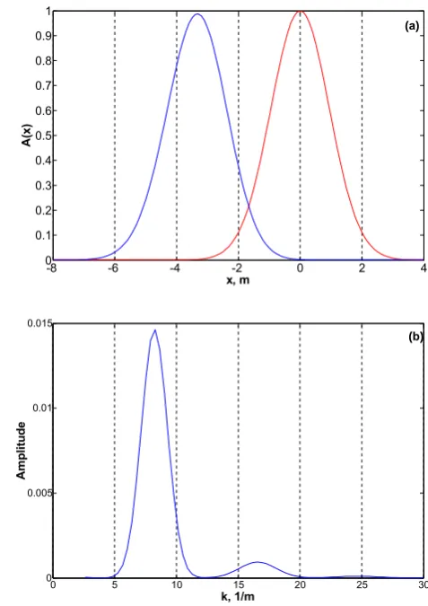
While Eqs. (20)–(21) represent the solution of the spatial evolution problem; they describe the complex group enve-lope variation in time and space, and thus can be used to define the initial conditions for the solution of the temporal evolution problem. The calculated according to Eq. (21) en-velope shape is presented in Fig. 1a at two instants. The 1st curve corresponds to the instant when the maximum of the envelope is at the wavemaker located atx=0. The 2nd curve represents the spatial distribution of the group envelope im-mediately before the entrance of the group to the tank and corresponds to the instant when the wave group excitation by the wavemaker is initiated in the experiments. This wave envelope is somewhat wider than the 1st one, with the maxi-mum value below unity. This complex envelope shape prior to the group’s “entrance” to the tank served as the initial con-dition. Time in the present study is thus measured relative to that instant of initiation of the wavemaker movement. The wavenumber spectrum of the surface elevation presented in Fig. 1b apparently does not vary in time for the linearized problem and therefore can be seen as the initial spectrum for the nonlinear evolution problem.
The Dysthe model describing either the spatial or the tem-poral evolution of a nonlinear wave group is solved using the pseudo-spectral split-step Fourier method based on Lo and Mei (1985). The computed complex envelope is then trans-lated into the physical coordinates (x, t ). The variation of
21
-8 -6 -4 -2 0 2 4
0 0.1 0.2 0.3 0.4 0.5 0.6 0.7 0.8 0.9 1
x, m
A(
x)
(a)
0 5 10 15 20 25 30
0 0.005 0.01 0.015
k, 1/m
A
m
pl
it
ude
(b)
Figure 1. Initial conditions for the temporal evolution computations. A) Envelope shape
centered at the wavemaker (x=0 m) and at the instant corresponding to imitation of the
wavemaker operation (Fig. 1. Initial conditions for the temporal evolution computations.t=0 s); b) Initial wavenumber amplitude spectrum. (a) Envelope shape centered at the wavemaker (x=0 m) and at the instant corresponding to initiation of the wavemaker operation; (b) Initial wavenumber amplitude spectrum.
the surface elevation at any fixed locationη(x0,t )in the
spa-tial formulation, or at the fixed instantη(x,t0)in the
tempo-ral formulation, is obtained from the complex envelope that contains the 2ndorder correction calculated using Eq. (16).
4 Video data processing
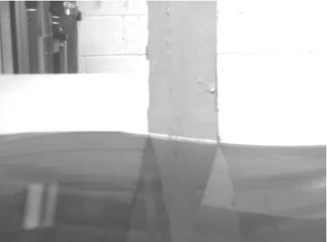
An example of a recorded image is presented in Fig. 2. While the contact line can be clearly identified visually, the image contains numerous additional features such as the tank sup-porting beam, objects in the laboratory beyond the tank, re-flections, etc. An effective algorithm was developed to ex-tract quantitative information from the recorded video clips that contain thousands of images like that in Fig.2.
22
F
Figure 2. Contact line image that contains tank wall supporting beam and the viewing window Fig. 2. Contact line image that contains tank wall supporting beam
and the viewing window.
area is cropped from the whole image in the vicinity of the desired curve as a rectangular window that is small with re-spect to the entire image. The initial window is built in the 1st image of the series around a point that constitutes the center of the searching area and is chosen at or in a close vicinity to the desired curve. Since the slope of the interface is usually quite small, the window aspect ratio selected in most cases is in the range of 2 to 3, with the width of the window being about 50 pixels.
The vertical coordinate of the interfacial curve for every horizontal location is defined as the weighted average of the pixel intensities along the vertical extent of the window. Once all vertical coordinates within the window are calcu-lated, contact line shape within the window is approximated by a second order polynomial using the least mean square fit on the array of the detected points. The vertical coordi-nate of the contact line at the center of the window is finally obtained from the polynomial value at the corresponding hor-izontal coordinate. The contact line coordinates determined by this procedure contain contribution of the pixel intensities in the vicinity of each point and are obtained at a sub-pixel resolution.
The window is then shifted forward by one pixel in the di-rection given by the slope of the contact line, and the process is repeated. At each step, the window is inclined by an angle corresponding to the window shift direction. This process continues until the whole image is covered. Once the coor-dinates of the contact line profile in a given frame have been determined, the search in the next frame is performed utiliz-ing this information. At the recordutiliz-ing rate of 30 frames per second, the contact line shift between the consecutive frames is quite small, making it advantageous to start the search in the next frame with the initial window built around the pre-vious profile.
The applied procedure has an additional advantage of al-lowing processing of numerous clips captured during the ex-periment at different locations along the tank automatically. At various locations along the tank the vertical position of the camera and its distance from the opposite tank wall re-main constant within a reasonable accuracy. Each clip was recorded after the camera has been shifted along the tank by the distance corresponding to the horizontal extent of the recorded image, and the wavemaker was activated after a suf-ficient delay so that all waves from the previous run have vanished. The initial search window in the consecutive clips is placed according to the coordinate of the interface deter-mined in the last window of the clip recorded at the upstream location at the identical timing relative to the reference sig-nal.
The present experimental approach was validated exten-sively using conventional resistance wire gauges at a number of locations along the tank and comparing with data simul-taneously acquired at same distancex by image processing technique. Measurements of the evolution of wave groups with wide frequency spectra that vary significantly along the tank due to dispersion and nonlinearity (Shemer et al., 2007) were performed for validation purposes. The spanwise uni-formity of the surface elevation was also checked by placing the probes across the tank. The difference between the in-stantaneous values of the surface elevation measured by the wave gauge located close to the tank’s wall and by video im-age processing at various distances from the wavemaker al-ways remains well below 1 mm and does not exceed the de-viation between the outputs of different probes. The spectra derived from those measurements exhibit a very good agree-ment for all frequencies in the spectra. More details on the experimental method employed are given in Dorfman and Shemer (2007).
5 Experimental and numerical results
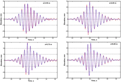
The temporal variation of the surface elevation within a wave group with the initially Gaussian envelope at x=0 as given by Eqs. (17) and (18) is studied first. Variation of the surface elevation within the group at a number of locations along the tank computed according to Eqs. (11)–(14) is compared in Fig. 3 with the results of video image processing.
23
22 24 26 28 30 32
-30 -20 -10 0 10 20 30
Time, s
E
levatio
n
, m
m
x=3.55 m
Figure 3. Variation of the surface elevation within the group at different distances x from the wavemaker): experiments; simulations
26 28 30 32 34 36
-30 -20 -10 0 10 20 30
Time, s
E
le
vat
io
n
, m
m
x=5.75 m
28 30 32 34 36 38
-30 -20 -10 0 10 20 30
Time, s
E
le
vat
io
n
, m
m
x=6.85 m
24 26 28 30 32 34
-30 -20 -10 0 10 20 30
Time, s
E
levat
io
n, m
m
x=4.65 m
Fig. 3. Variation of the surface elevation within the group at different distancesxfrom the wavemaker:—experiments;—simulations.
clearly demonstrates that the duration of the group extends withx and that the initially symmetric Gaussian envelope shape (Fig. 1a) gradually exhibits stronger left-right asym-metry, with increasingly steep front and elongated tail. The maximum surface elevation within the group may exceed significantly the nominal value ofa0. This increase of the
maximum amplitude is associated in part with the focusing properties of the nonlinear Schr¨odinger equation that affects the shape of the group envelope, as discussed in Shemer et al. (1998). The NLS equation, however, is only capable of reflecting correctly some limited features of the solution, and the extension to the MNLS equation is required to get both qualitative and quantitative agreement between experiments and computations, see Shemer et al. (2002). Ap apparent additional reason for higher maximum values of the surface elevation notable in Fig. 3, as well as for the crest-trough asymmetry, is the contribution of 2nd order bound (locked) waves.
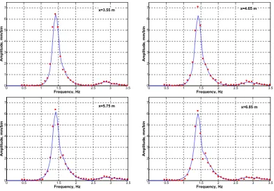
The notable variation of the group shape along the tank in Fig. 3 is due to both linear dispersion and nonlinear ef-fects. To separate linear and nonlinear contributions, fre-quency spectra of surface elevation variation in time that vary only due to nonlinear effects, are presented in Fig. 4. The frequency spectra of Fig. 4 are plotted for the same loca-tions along the tank as in Fig. 3. The spectra are computed for those parts of the surface elevation records that contain the whole group with duration of about 13 s (about 20T0).
The spectra are thus discrete with the frequency increment of
about 0.077 Hz. For demonstration purposes only, the ampli-tude spectra obtained for the computed temporal variation of the surface elevation that naturally are smoother than the re-sults derived from the experimental data, are drawn as a solid line.
The agreement between experiments and computations in Fig. 4 is quite good. While the initial amplitude spectrum corresponding to Eq. (17) also has a symmetric Gaussian shape, the spectra of Fig. 4 are asymmetric and deviate from the Gaussian shape. Note the existence of a kink in the spec-tral shape at the frequency slightly exceeding the dominant one, f0=1/T0=1.43 Hz, that is visible atx=5.75 m and
be-comes stronger atx=6.85 m. The kink is observable both in the measured and in the computed spectra. Even for a rel-atively short extent of the spatial evolution, widening of the spectrum is visible in Fig. 4. This spectral widening and non-Gaussian spectral shape indicate that nonlinearity is essential in the wave group evolution along the tank.
The contribution of the 2nd order bound waves to the am-plitude spectrum is quite significant at all locations. The measured using the digital processing of the video images spectrum of bound waves around the 2nd harmonic of the dominant frequency f0 is in excellent agreement with the
24 Figure 4. Variation of the frequency spectra along the tank: symbols– experiments, line – simulations
0 0.5 1 1.5 2 2.5 3 3.5
0 1 2 3 4 5 6 7
Frequency, Hz
Am
p
lit
ud
e,
m
m
/b
in
x=4.65 m
0 0.5 1 1.5 2 2.5 3 3.5
0 1 2 3 4 5 6 7
Frequency, Hz
Am
p
lit
u
d
e, m
m
/b
in
x=3.55 m
0 0.5 1 1.5 2 2.5 3 3.5
0 1 2 3 4 5 6 7
Frequency, Hz
Am
p
lit
ud
e,
m
m
/b
in
x=5.75 m
0 0.5 1 1.5 2 2.5 3 3.5
0 1 2 3 4 5 6 7
Frequency, Hz
Am
p
lit
ud
e,
m
m
/b
in
x=6.85 m
Fig. 4. Variation of the frequency spectra along the tank: symbols – experiments, line – simulations.
As stressed above, the main motivation for developing the data acquisition method based on the processing of se-quences of video images is in its capability to measure in-stantaneous spatial distribution of the surface elevation. Ap-plication of this method enables following the temporal evo-lution of the whole wave group as well. This information can be compared with the numerical solution of the system of Eqs. (7)–(10) that constitute the Dysthe model in its tem-poral formulation. The initial conditions for the temtem-poral evolution caseA(x, 0) are obtained using Eqs. (21) and (22), as described in Sect. 3 and presented in Fig. 1.
To compare the numerical and the experimental results, the whole group at the selected instants has to be physically present within the wave tank boundaries. The numerical so-lution of Eqs. (7)–(10) indicates that at the dimensional time
t=12 s (relative to the instant depicted in Fig. 1) the advance-ment of the group along the tank is sufficient for the tail of the computed instantaneous spatial envelope distribution to emerge within the tank, thus enabling comparison with the experiment. Similarity of the numerical and the experimental results is examined also at three additional instants:t2=14 s; t3=16 s andt4=18 s. Equations (15)–(16) are used again to
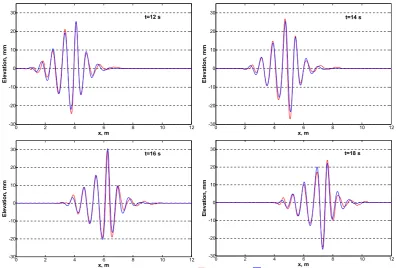
account for the contribution of the 2nd order bound waves. The spatial variation of the surface elevation as a result of the temporal evolution of the complex wave envelope is pre-sented at the selected instances in Fig. 5. As in the spatial evolution case, good agreement is obtained between the nu-merical simulations and the experimental observations. At the earliest instant presented in Fig. 5,t=12 s, the formation
of the group has just been completed and the group in its en-tirety emerges in the tank, while at the last instant,t=18 s, the front of the group approaches the far end of the wave tank.
Deviation of the group shape in Fig. 5 from the initial en-velope presented in Fig. 1a is obvious. Both left-right and trough-crest asymmetries observed in the temporal records presented in Fig. 3, as well as significant variations in the extreme values of the surface elevation within the group, are visible in Fig. 5 as well. Note, however, that the left-right asymmetry in Fig. 5 is opposite to that of Fig. 3, where the steeper part of the group appears at earlier sampling times. The experimental results are in agreement with the numeri-cal solutions of the temporal Dysthe model.
Comparison of Figs. 3 and 5 also illustrates the well known fact that since the group velocity of deep water waves is a half of their phase velocity, the number of waves within the group in the temporal surface elevation variation records of Fig. 3 is twice larger than in the instantaneous spatial “snapshots” of the same group plotted in Fig. 5.
25
0 2 4 6 8 10 12
-30 -20 -10 0 10 20 30
x, m
E
levat
io
n
, m
m
t=12 s
0 2 4 6 8 10 12
-30 -20 -10 0 10 20 30
x, m
E
levat
io
n
, m
m
t=14 s
Figure 5. The instantaneous surface elevation at various instants: experiments; simulations
0 2 4 6 8 10 12
-30 -20 -10 0 10 20 30
x, m
E
le
vat
io
n,
mm
t=18 s
0 2 4 6 8 10 12
-30 -20 -10 0 10 20 30
x, m
E
le
vati
o
n
, mm
t=16 s
Fig. 5. The instantaneous surface elevation at various instants:—experiments;—simulations.
26 Figure 6. Wavenumber spectra of the surface elevation at various instants: symbols – experiments; lines - simulation
0 5 10 15
0 1.5 3 4.5
k, 1/m
Am
p
lit
u
d
e,
m
m
/b
in
Experiment Free + Bound Waves Free Waves only Bound Waves only t=12 s
0 5 10 15
0 1.5 3 4.5
k, 1/m
A
m
p
litude, m
m
/bi
n
t = 14 s
0 5 10 15
0 1.5 3 4.5
k, 1/m
A
m
plit
ude
, m
m
/bin
t = 16 s
0 5 10 15
0 1.5 3 4.5
k, 1/m
A
m
p
litude, m
m
/bi
n
t = 18 s
All spectra in Fig. 6 exhibit essential differences from the initial wavenumber spectrum presented in Fig. 1b. The agreement between the simulated and the experimental re-sults in Fig. 6 is quite good at all instances presented; the differences can be attributed in part to inaccuracy associated with choosing the initial condition. There are similarities but also essential differences between the frequency spec-tra given in Fig. 4, and the wave number specspec-tra of Fig. 6. In both figures the spectra become wider in the course of the wave group evolution. The wave number spectra in all frames of Fig. 6 are however much wider than the frequency spectra in Fig. 4.
The larger width of the wave number spectra relative to the frequency spectra follows from the dispersion relation for deep water, Eq. (1) that is appropriate for the present exper-iments. In the narrow spectrum approximation the relative widths of those spectra are related by
1k k0
=21ω
ω0
(23) As a result, in all frequency spectra of the temporal variation of the surface elevation for a narrow-band wave group mov-ing along the tank, Fig. 4, the free waves and the bound waves are totally separated. For the initial condition presented in Fig. 1b, the separation of free and bound waves’ spectral do-mains still exists. The spectral widening in course of group propagation along the tank, however, leads to overlapping domains of the free and of the 2nd harmonic bound waves in the wave number spectra of Fig. 6. Each measured spectrum apparently contains free as well as bound waves. In numeri-cal simulations, complex group envelope that corresponds to free waves only is computed first. Bound waves are then ob-tained from the free wave field. The computed wave number spectra of free and bound waves are also plotted in Fig. 6.
The overlapping of free and bound waves domains in the wave number spectra precludes straightforward filtering out of the free wave spectrum from the experimental results. This difficulty complicates significantly the determination of the spatial group envelope’s shape that contains the free-wave part only from the experimental data. The initial conditions for solving the temporal evolution problem could not there-fore be determined from experiment. This difficulty forced to apply the linearized approach presented by Eqs. (19)–(22) in order to translate the temporal variation of the surface el-evation at the wavemaker given by Eqs. (17), (18) into the spatial form.
Accounting for the 2nd harmonic bound waves is essen-tial to get a better agreement with the measured spectra at high wave numbers. The disagreements between computa-tions and measurements in the low wave number region of the spectrum in Fig. 6 may partially stem from the fact that for longer waves, the depth of the experimental facility of 0.6 m is not large enough for those wave components to be considered deep. The low wave number bound waves may become significant and can constitute a significant
contribu-tion to the spectral shape. The effect of long bound waves was considered in the framework of the Zakharov equation in Shemer et al. (2007). The validity of Dysthe equation that served as the theoretical model in the present study, how-ever, is restricted to deep waves. The long bound waves were therefore not considered in the current study.
6 Discussion
It should be stressed that theoretical studies of nonlinear water-waves are often performed by solving temporal evo-lution models, while in the laboratory as well as in field experiments surface elevation variation with time is usually recorded at fixed locations, sometimes these data also contain information on the wave propagation directions. Attempts are sometimes made to translate the measured by point sen-sors frequency spectrum into the corresponding wave num-ber (or wave vector in the two-dimensional case) spectrum. However, direct quantitative comparison of the frequency and the wave number spectra can not be carried out in a con-sistent way.
Instantaneous “snapshot” of the whole wave field taken to get the wave number spectrum, on one hand, and measure-ments of the temporal variation of the surface elevation vari-ation with time at a fixed locvari-ation to get the wave frequency spectrum, on the other hand, constitute essentially different ways of studying an evolving in space and in time water-wave field. Moreover, as the present study demonstrates, direct computation of the wave number spectrum from the measured frequency spectrum can not be carried out even assuming that the evolution is slow as compared to the rel-evant temporal scale (represented by the duration of contin-uous sampling that determines the frequency resolution of the spectrum) and the spatial scale (the extent of the imaged wave field that determines the wave number spatial resolu-tion) of the data acquisition process.
to evaluate quantitatively the shape of the high end of the wave number spectrum from the measured surface elevation variation in time at a fixed location and the corresponding frequency spectrum.
Two version of the MNLS equation are considered here: The first is based on the original formulation of Dys-the (1979), Eqs. (7) to (10), that describes evolution in time of a unidirectional narrow-spectrum wave group with pre-scribed initial spatial distribution of the complex group en-velope. Lo and Mei (1985) were the first to notice that in order to carry out comparison with experimental data pro-vided by point sensors, a version of the MNLS equation that describes evolution of the wave group envelope in space is re-quired. The spatial version introduced in their paper requires prescribed temporal variation of the complex wave envelope at a given location, usually at the wavemaker, as the initial condition.
Each version of the MNLS equation, either spatial or tem-poral, yields variation of the wave field in time as well as in space. The derivation of the spatial MNLS version by Lo and Mei was based on the temporal Dysthe equation and the appropriate change of variables. The two version of the MNLS equation can also be derived from the correspond-ing temporal (Stiassnie, 1984; Hogan, 1986) or spatial (Kit and Shemer, 2002) versions of the Zakharov equation. These derivations shed light on two important facts. First, the evo-lution equations for complex envelopes of the surface ele-vation variation and for the velocity potential are somewhat different at the 4th order appropriate for the MNLS model. Since the surface elevation is the parameter measured di-rectly, the surface elevation version of the MNLS equation is used here for carrying out quantitative comparison of model predictions with the experimental results.
The second comment is related to the inclusion of ad-ditional linear terms in the temporal version of the MNLS equation by Trulsen and Dysthe (1996) and Trulsen et al. (2000). Derivation of the Dysthe model from the Za-kharov equation clearly demonstrates that these additional terms appear due to expansion of the interaction coefficient in the Zakharov equation around the carrier wave frequency
ω0in terms of the wave number deviation fromk0. For
uni-directional waves in deep water this expansion has an infinite number of terms and therefore has to be truncated. In the spatial evolution case the situation is different and the expan-sion is of the wave numbers around the frequencyω0. For the
dispersion relation presented by Eq. (1) the expansion does not contain terms beyond quadratic. In the spatial version of the unidirectional MNLS the dispersion is thus presented ex-actly. The spatial evolution version of the MNLS equation is therefore more accurate in this sense than the temporal ver-sion.
7 Conclusions
An effective method for identification of the instantaneous contact line shapes in a sequence of recorded video images is developed. Experiments indicate that the surface eleva-tion values calculated employing the proposed image-based method have an error comparable to that of conventional re-sistance type gauges.
Advantage was taken of the controlled and repeatable character of the experiments that enabled synchronization of the video camera and the wavemaker operation to ob-tain phase-locked surface elevation distributions on length scales exceeding the size of the imaged scene. The applied technique allows studying temporal evolution of the instanta-neous wave field in the whole tank and thus determination of the variation in time of the wavenumber spectra. This ability is important for carrying out quantitative comparison of pre-diction of nonlinear evolution models with the experimental results.
This experimental approach is adopted here to study both the spatial and the temporal evolution of narrow-banded uni-directional wave groups. The experimental results are com-pared in detail with the solutions of the appropriate version of the MNLS equation. The present experimental and numeri-cal study demonstrates that the envelopes of deep-water uni-directional wave groups with narrow spectrum have certain similarities in their evolution pattern in both time and space. Good quantitative and qualitative agreement between mea-surements and computations is obtained for both the spatial and the temporal evolution formulations. The most visible feature of the evolution process is the gradual transforma-tion of the initially symmetric envelope shape into a strongly asymmetric one. This feature can not be reproduced by the cubic Schr¨odinger equation in which the initially symmetric envelope can not become asymmetric, and requires the ex-tension to the MNLS equation for its proper description.
Both the spatial and the temporal version of the model de-scribe correctly the widening of the spectrum in the course of evolution. The shapes of the spectra are, however, quite different in these formulations, the wave number spectrum being twice wider than the corresponding frequency spec-trum.
Acknowledgement. The support of this study by a grant # 964/05 from the Israel Science Foundation is gratefully acknowledged.
Edited by: V. Shrira
Reviewed by: two anonymous referees
References
Benjamin, T. B. and Feir, J. E.: The disintegration of wavetrains on deep water, J. Fluid Mech., 27, 417–430, 1967.
Dean, R. G. and Dalrymple, R. A.: Water wave mechanics for engi-neers and scientists, World Scientific, Singapore, 1991. Dorfman, B. and Shemer, L.: Video image-based technique for
measuring wave field evolution in a laboratory wave tank, Mar-itime Industry, Ocean Eng. and Coastal Resources, 2, edited by: Guedes Soares, C. and Kolev, P. K., Taylor & Francis, London, 711–720, 2007.
Dysthe, K. B: Note on a modification to the nonlinear Schr¨odinger equation for application to deep water waves, Proc. R. Soc. Lond., A369, 105–114, 1979.
Hasimoto, H. and Ono, J.: Nonlinear modulation of gravity waves, J. Phys. Soc. Japan, 33, 805–811, 1972.
Hogan, S. J.: The potential form of the fourth-order evolution equa-tion for deep-water gravity-capillary waves, Phys. Fl., 29, 3479– 3480, 1986.
Kit, E. and Shemer, L.: Spatial versions of the Zakharov and Dysthe evolution equations for deep water gravity waves, J. Fluid Mech., 450, 201–205, 2002.
Lake, B. M., Yuen, H. C., Rungaldier, H., and Ferguson, W. E.: Nonlinear deep water waves: theory and experiment, 2. Evolu-tion of a continuous wave train, J. Fluid Mech., 83, 49–74, 1977. Lo, E. and Mei, C. C.: A numerical study of water-wave modulation based on a higher-order nonlinear Schr¨odinger equation, J. Fluid Mech., 150, 395–416, 1985.
Pelinovsky, E. and Kharif, C.: Simplified model of the freak wave formation from the random wave field, Proc. 15th Int. Workshop on Water Waves and Floating Bodies, edited by: Miloh, T. and Zilman, G. Caesaria, 142–145, 2000.
Shemer, L., Kit, E., Jiao, H.-Y., and Eitan, O.: Experiments on nonlinear wave groups in intermediate water depth, J. Waterway, Port, Coastal & Ocean Eng., 124, 320–327, 1998.
Shemer, L., Jiao, H.-Y., Kit, E., and Agnon, Y.: Evolution of a non-linear wave field along a tank: experiments and numerical sim-ulations based on the spatial Zakharov equation, J. Fluid Mech., 427, 107–129, 2001.
Shemer, L., Kit, E., and Jiao, H.-Y.: An experimental and numerical study of the spatial evolution of unidirectional nonlinear water-wave groups, Phys. Fl., 14, 3380–3390, 2002.
Shemer, L., Goulitski, K., and Kit, E.: Evolution of wide-spectrum wave groups in a tank: an experimental and numerical study, Eur. J. Mech. B/Fluids, 26, 193–219, 2007.
Stiassnie, M.: Note on the modified nonlinear Schr¨odinger equation for deep water waves, Wave Motion, 6, 431–433, 1984. Trulsen, K. and Dysthe, K. B.: A modified nonlinear Schr¨odinger
equation for broader bandwidth gravity waves on deep water, Wave Motion, 24, 281–289, 1996.
Trulsen, K., Kliakhandler, I., Dysthe, K. B., and Velarde, M. G.: On weakly nonlinear modulation of waves on deep water, Phys. Fl., 12, 2432–2437, 2000.
Yuen, H. C. and Lake, B. M.: Nonlinear deep water waves: Theory and experiment, Phys. Fluids, 18, 956–960, 1975.