www.ocean-sci.net/4/151/2008/
© Author(s) 2008. This work is distributed under the Creative Commons Attribution 3.0 License.
Ocean Science
The low-resolution CCSM2 revisited: new adjustments and a
present-day control run
M. Prange
MARUM – Center for Marine Environmental Sciences and Department of Geosciences, University of Bremen, Klagenfurter Str., 28334 Bremen, Germany
Received: 26 July 2006 – Published in Ocean Sci. Discuss.: 18 August 2006 Revised: 17 April 2008 – Accepted: 18 April 2008 – Published: 26 May 2008
Abstract. The low-resolution (T31) version of the Com-munity Climate System Model CCSM2.0.1 is revisited and adjusted by deepening the Greenland-Scotland ridge, chang-ing oceanic mixchang-ing parameters, and applychang-ing a regional freshwater flux adjustment at high northern latitudes. The main purpose of these adjustments is to maintain a robust Atlantic meridional overturning circulation which collapses in the original model release. The paper describes the present-day control run of the adjusted model (referred to as “CCSM2/T31x3a”) which is brought into climatic equi-librium by applying a deep-ocean acceleration technique. The accelerated integration is extended by a 100-year syn-chronous phase. The simulated meridional overturning cir-culation has a maximum of 14×106m3s−1in the North At-lantic. The CCSM2/T31x3a control run is evaluated against observations and simulations with other climate models. Most shortcomings found in the CCSM2/T31x3a control run are identified as “typical problems” in global climate modelling. Finally, examples (simulation of North Atlantic hydrography, West African monsoon) are shown in which CCSM2/T31x3a has a better simulation skill than the latest low-resolution Community Climate System Model release, CCSM3/T31.
1 Introduction
Transporting cold deepwater from the North Atlantic to the Southern Ocean and warm water masses in the upper lay-ers in opposite direction, the present-day Atlantic merid-ional overturning circulation (AMOC) is associated with a substantial northward heat transport of order 1015W (e.g. Ganachaud and Wunsch, 2000). During the past two decades
Correspondence to: M. Prange
of paleoceanographic and paleoclimatic research the role of the AMOC in driving or amplifying global climatic changes came more and more into focus. Strong variations in the AMOC might have induced changes in the global temper-ature distribution, wind fields and the hydrologic cycle. The possibility that the AMOC could change in the future (Meehl et al., 2007) motivates paleoceanographers to understand how it may have differed in the past.
Fig. 1. Atlantic meridional overturning circulation (Sv) obtained
with the Eulerian-mean velocity from the standard CCSM2/T31 control run with default settings and parameters. A 10-yr average is shown calculated from years 278–287 (the control run has started from observational data).
their climatic effect relied on the perturbation of North At-lantic Deep Water (NADW) formation by melting icebergs (e.g. Rahmstorf, 2002, and references therein). Freshwater perturbations in the North Atlantic were also likely to be responsible for the last two pronounced cold intervals, the Younger Dryas (ca. 13 000 years ago) and the “8 k event” about 8200 years ago (Alley and Agustsdottir, 2005, and ref-erences therein). Less pronounced Holocene climatic shifts in the North Atlantic realm have recently been associated with moderate AMOC variations (Oppo et al., 2003; Schulz et al., 2007; Jongma et al., 2007). These few examples demonstrate that the AMOC is crucial for the understanding of past – and probably future – climate change. A climate model without representation of the AMOC is virtually use-less for most paleo-relevant scientific questions.
Paleoclimatic model experiments usually require long in-tegration times either to reach climatic equilibria which differ from the present-day situation or to simulate long-term (e.g. millennial) climatic trends and changes. To reduce computa-tion time, numerical models used in paleoceanographic and paleoclimatic research are therefore often reduced in com-plexity (cf. Claussen et al., 2002) and/or employ relatively coarse grid resolutions. Low-resolution configurations of the fully-coupled NCAR (National Center for Atmospheric Research) Community Climate System Model CCSM have been released both for version 2.0.1 (“CCSM2/T31”) and for version 3.0 (“CCSM3/T31”). In these so-called “paleo versions”, the horizontal resolution of the atmospheric com-ponent is given by T31 spectral truncation (3.75◦by 3.75◦ transform grid), whereas the ocean has a nominal resolu-tion of 3.6◦ by 1.6◦with 25 levels. While the present-day control run of CCSM3/T31 exhibits a robust thermohaline circulation in the Atlantic Ocean (Yeager et al., 2006), the AMOC spins down in CCSM2/T31 such that the net
vol-could contribute to the improvement of the AMOC simula-tion as well (albeit more indirectly). Either way, there seems to be no obvious reason why CCSM2/T31 should not be consigned to history in view of the release of CCSM3/T31. In the present paper, however, it is shown that the perfor-mance of CCSM2/T31 can substantially be improved by ap-plying some modifications to the original model. The low-resolution version of CCSM2.0.1 with these adjustments in-cluded is referred to as CCSM2/T31x3a to reflect the at-mospheric resolution (“T31”), the average resolution of the ocean grid (“x3”) as well as the implementation of ad-justments (“a”). We shall see that CCSM2/T31x3a simu-lates a robust AMOC that is similar to the ocean circula-tion in CCSM3/T31. Even more interesting, there are sev-eral applications where CCSM2/T31x3a performs better than CCSM3/T31, depending on the phenomenon under investi-gation and its geographical location.
The present paper is devoted to the description of the present-day control run of CCSM2/T31x3a. Even though a detailed model intercomparison is far beyond the scope of this paper, examples shall be shown in which CCSM2/T31x3a provides a better simulation than CCSM3/T31. The following section describes the tuning of CCSM2/T31x3a. Section 3 describes and discusses the asyn-chronous integration technique which is used to achieve a statistical equilibrium climate state. The present-day climate from the CCSM2/T31x3a control run is presented in Sect. 4. The focus is placed on oceanic and atmospheric climatolog-ical means. The simulation skill for interannual variability in the tropical Pacific and North Atlantic regions is briefly discussed. CCSM2/T31x3a’s control run is compared with other models – particularly with CCSM3/T31 – in Sect. 5. Conclusions are drawn in Sect. 6.
2 CCSM2/T31x3a: components and adjustments
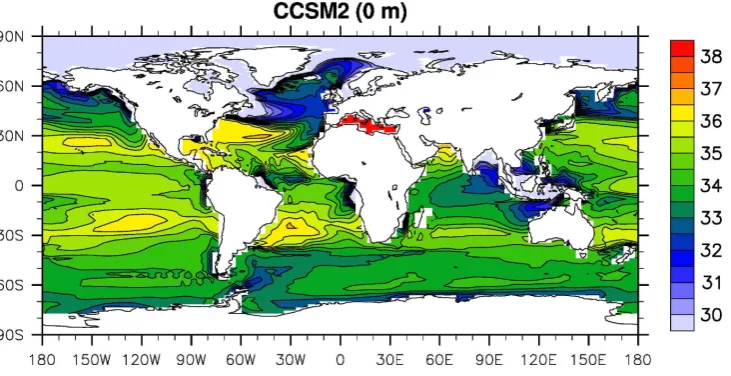
Fig. 2. Annual-mean sea surface salinity (psu) in the standard CCSM2/T31 control run with default settings and parameters. A 10-yr average
is shown calculated from years 278–287 of the simulation. The model output can be compared with observations shown in Fig. 14.
via a central coupler. The atmosphere component is the Com-munity Atmosphere Model CAM2, a global general circula-tion model developed from NCAR’s CCM3 (Collins et al., 2003). CAM2 employs a spectral dynamical core (i.e. the numerical solutions of the partial differential equations are approximated using harmonics and involve the use of the Fast Fourier Transform; e.g. Canuto et al., 1988) and hy-brid vertical coordinates with 26 levels, combining terrain-following sigma coordinates (which are defined by the ratio of the pressure at a given point in the atmosphere to the pres-sure on the surface of the earth underneath it) at the bottom with pressure-level coordinates at the top of the model. The ocean is represented by the z-coordinate, Bryan-Cox type (cf. Kantha and Clayson, 2000) Parallel Ocean Program POP 1.4 (Smith and Gent, 2002). The model employs an implicit free surface (Dukowicz and Smith, 1994), an anisotropic vis-cosity parameterization (Smith and McWilliams, 2003) and Gent and McWilliams’ (1990) isopycnal mixing for tracers using the skew-flux form (Griffies, 1998). A non-local KPP (K-profile parameterization) scheme is applied for vertical mixing (Large et al., 1994). The sea-ice component is the Community Sea-Ice Model CSIM4 (Briegleb et al., 2002) with elastic-viscous-plastic dynamics scheme (Hunke and Dukowicz, 1997), an explicit brine-pocket parameterization (Bitz and Lipscomb, 1999) and an ice thickness distribution module that accounts for five ice thickness categories (Bitz et al., 2001). The land component of CCSM2.0.1 is the Com-munity Land Model CLM2 (Vertenstein et al., 2002). It in-cludes complex biogeophysics and hydrology along with a state-of-the-art river runoff module (Branstetter and Erick-son, 2003). Detailed documentations of all model compo-nents and parameters can be found at www.ccsm.ucar.edu/ models/ccsm2.0.1.
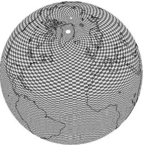
In the framework of CCSM, atmosphere and land models share an identical horizontal grid. Likewise, ocean and sea ice use one and the same horizontal grid. In CCSM2/T31x3a, the ocean/sea-ice component is formulated on an orthogonal grid which shifts the north pole singularity into Greenland to avoid time-step constraints due to grid convergence. This grid is referred to as “gx3v4” (Fig. 3). It has a longitudinal resolution of 3.6◦. The latitudinal resolution of “gx3v4” is variable, with finer resolution (approximately 0.9◦) near the equator.
In CCSM2/T31x3a, several adjustments to the standard CCSM2.0.1 release are applied. The overall goal is to am-plify the meridional overturning circulation in the Atlantic Ocean. Due to the computational expense of performing fully-coupled experiments systematic sensitivity studies, elu-cidating the effects of each modification separately, are not feasible for the time being. The tuning of CCSM2.0.1 is based on experience with other models. CCSM2/T31x3a in-cludes the following adjustments:
– The Greenland-Scotland ridge is slightly deepened such that the sill depths are∼590 m and∼900 m in the Den-mark Strait and in the Iceland-Scotland passage, respec-tively (Fig. 4). Given the rather coarse resolution of the “gx3v4” ocean grid, the new bathymetry is still appro-priate. A deeper Greenland-Scotland ridge facilitates the exchange of dense water masses between the North Atlantic and the Nordic Seas where deep winter convec-tion takes place (cf. Koesters et al., 2004).
Fig. 3. Horizontal cell distribution of the ocean/sea-ice grid “gx3v4”. Note the displaced north pole and the enhanced resolu-tion at low latitudes.
0.3 cm2/s is reached at about 2300 m depth). Thus, com-pared to the default setting, vertical mixing is slightly increased in the upper ocean below the surface bound-ary layer (alternatively, one could have applied geo-graphically varying upper-ocean parameters with lower vertical diffusivity in the tropics and much higher values in the Southern Ocean where internal wave activity is known to be enhanced, see Gnanadesikan et al., 2006). Vertical mixing provides a mechanism for the conver-sion of cold deep waters into warm water of the upper layers. The crucial role of vertical mixing in driving the thermohaline circulation has been demonstrated in nu-merous studies (e.g. Bryan, 1987; Wright and Stocker, 1992; Marotzke, 1997; Prange et al., 2003).
– For the Redi and bolus parts of the Gent-McWilliams parameterization diffusivities are set to 1.2×107cm2/s. This represents a 50% increase compared to the default. It is expected that higher horizontal mixing counter-acts halocline formation in the northern North Atlantic, thereby favouring convective activity and NADW for-mation (cf. Schmittner and Weaver, 2001).
– The coefficient used in the quadratic ocean bottom drag formula is increased from 10−3to 10−2. The most im-portant effect of this change is a substantial retardation of the flow through the shallow Bering Strait. This throughflow is associated with an import of relatively fresh water from the North Pacific to the Arctic Ocean
are potentially important for NADW formation. Be-yond these regions, the hydrological cycle is simulated without unphysical adjustments. This is a main advan-tage over the more common application of global flux-correction fields. The freshwater flux redistribution re-quires modifications in the POP Fortran code and it is presumably the most substantial change to the standard model set-up. Note that neither heat nor momentum flux corrections are implemented in CCSM2/T31x3a. In addition to the model tuning which aims at boosting the AMOC, optimized sea-ice/snow albedos are applied based on results from stand-alone sea-ice model experiments: Max-imum albedos for thick, dry sea ice are set to 0.82 and 0.38 for the visible and near-infrared spectral band, respectively. The near-infrared albedo for dry snow is set to 0.74. No dis-tinction is made between the hemispheres.
3 Accelerated integration
Accelerated integration techniques are often applied to cli-mate models to reduce the computational expense. In or-der to obtain a present-day climatic equilibrium, a deep-ocean acceleration technique – which is highly efficient in the framework of CCSM2/T31x3a – is employed here. This ap-proach allows for increasing tracer time steps with depth, ex-ploiting the relaxation of the Courant-Friedrichs-Lewy con-straint due to diminishing current speeds in the deep ocean (Bryan and Lewis, 1979; Bryan, 1988). Such an asyn-chronous integration technique has proven useful for search-ing equilibrium solutions without any interest in the transient behaviour of the model: Once an equilibrium is reached (i.e. vanishing time-derivates in the model equations), the solu-tion is independent of the time-stepping.
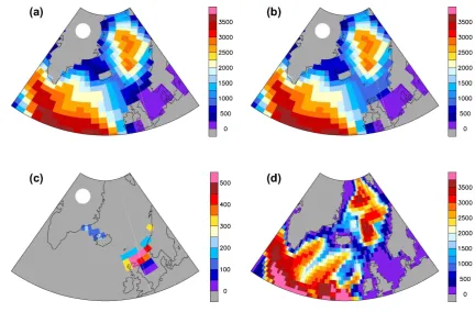
Fig. 4. Bathymetry around the Greenland-Scotland ridge: (a) Ocean depths (m) at tracer grid points in the original low-resolution CCSM2.0.1 release plotted in raster-mode to display the “gx3v4” ocean-grid structure; (b) same as (a) but for the new bathymetry used in CCSM2/T31x3a; (c) difference between CCSM2/T31x3a and original bathymetry; (d) real bathymetry (ETOPO60) for comparison.
in a realistically forced ocean model due to intra- and inter-annual variability. In order to quantify these errors, Danaba-soglu (2004) recently applied accelerated integration meth-ods to POP 1.4 subject to realistic forcing. Comparing equi-librium temperatures and salinities obtained by deep-ocean acceleration with those from a 10 000-year synchronous con-trol run, he found that errors are of order 0.1 K and 0.1 psu, respectively, provided that two conditions are met: (i) verti-cal variations in time step are restricted to depths where ver-tical tracer fluxes (i.e. verver-tical gradients) are small enough that tracers are conserved well enough (in particular below the pycnocline); (ii) the accelerated integration is extended by a synchronous phase of – at least – several decades (Dan-abasoglu et al., 1996; Wang, 2001; Dan(Dan-abasoglu, 2004). The synchronous extension is important not only to correctly cap-ture oceanic variability, but also to test the stability and re-liability of the accelerated equilibrium solution (cf. Bryan, 1984; see also Sect. 4.1). Previous modelling studies have demonstrated the ability of acceleration techniques to reach an equilibrium paleoclimatic solution (e.g. see Huber and Sloan, 2001; Huber and Nof, 2006).
The acceleration-induced small errors found by Danaba-soglu (2004) are tolerable for most paleoclimatic applica-tions. In particular, errors in large-scale oceanic mass and heat transports turned out to be negligible (for instance, the
error in maximum Atlantic northward heat transport was about 0.01 PW or 1–2%). Using the same oceanic model grid as in the study by Danabasoglu (2004), a similar deep-ocean acceleration scheme is used here. The surface time step in the ocean model is set to 1 h (time-step restriction due to nu-merical instability) and does not change down to a depth of 1300 m. Below 2500 m, the tracer time step is increased by a factor 50. Between 1300 m and 2500 m, the tracer time step has a linear variation.
4 Present-day control run
4.1 Experimental design and spin-up
For the present-day control run of CCSM2/T31x3a, the at-mospheric composition of 1990 AD is adopted. Volume mix-ing ratios of greenhouse gases are listed in Table 1. The total aerosol visible optical depth is set to 0.14, while a value of 1365 W/m2 is used for the solar constant. The model is initialized with observational data sets provided at www.ccsm.ucar.edu/models/ccsm2.0.1.
Fig. 5. Sketch of the regional freshwater flux adjustment used in CCSM2/T31x3a. Surface freshwater fluxes by precipitation and river runoff into the ocean are reduced over the red area. The corre-sponding amount of freshwater is distributed over the Pacific Ocean (blue area). All other parts of the world ocean (yellow area) are not affected by the flux adjustment.
Table 1. Volume mixing ratios of greenhouse gases used in the
present-day control run.
Trace gas Volume mixing ratio
CO2 3.530×10⁻⁴ CH4 1.676×10⁻⁶ N2O 0.309×10⁻⁶ CFC11 0.263×10⁻⁹ CFC12 0.479×10⁻⁹
synchronous spin-up phase, depth-accelerated integration is applied for 293 years, followed by a centennial synchronous extension. This gives a total integration time of 400 surface years for the coupled climate model corresponding to 14,757 deep-ocean years. Only the third stage of the integration pro-cedure (i.e. the centennial synchronous phase) shall serve for an evaluation of the simulated present-day climate.
Figure 6 shows the time series of global ocean tempera-ture over the accelerated spin-up phase and the synchronous extension. Initialized with climatological data (Steele et al., 2001) the ocean cools by about 0.6 K until reaching a near-equilibrium state. During the same time, global average salinity increases by about 0.01 psu (not shown). This
salin-Fig. 6. Globally averaged potential temperature of the ocean
dur-ing spin-up, plotted as deviation from the mean value of year 400. Note that deep-ocean acceleration is applied from (surface) year 8 to (surface) year 300.
Table 2. Average maximum overturning strength (AMOC) and
peak northward heat transport (NAHT) in the North Atlantic, vol-ume transport through Drake Passage (ACC), Indonesian Through-flow (ITF), and Bering Strait throughThrough-flow (BS) in CCSM2/T31x3a. For comparison, estimates given by Ganachaud and Wunsch (G&W, 2000) and Stammer et al. (2003) are listed.
Transport CCSM2/T31x3a G&W Stammer
AMOC (Sv) 14 13–17 –
NAHT (PW) 0.6 1.15–1.45 0.6
ACC (Sv) 92 134–146 124
ITF (Sv) 10.5 11–21 11.5
BS (Sv) 1.3 0.8 –
ity drift is mainly attributable to the non-conservative char-acter of deep-ocean acceleration.
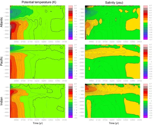
Fig. 7. Time versus depth (m) plots of horizontally averaged potential temperatures (left) and salinities (right) for the Atlantic, Pacific, and
Indian Ocean basins, plotted as deviations from the mean value of year 400 (smoothed by 7-yr averaging). Contour intervals are 0.1 K and 0.01 psu, respectively. Note that deep-ocean acceleration is applied from (surface) year 8 to (surface) year 300.
Starting from an ocean at rest, most mass (or volume) transports obtain quasi-equilibrium within 50 surface years. Figure 8 shows the temporal evolution of the Atlantic merid-ional overturning streamfunction at 25◦S. At equilibrium, al-most 12 Sv of deep water are exported to the Southern Ocean between 1000 and 3000 m depth; below 3000 m, 2–3 Sv of Antarctic Bottom Water (AABW) enter the Atlantic Ocean. The major goal of model tuning is achieved: CCSM2/T31x3a produces a robust AMOC which induces a substantial north-ward heat transport (cf. Sect. 4.2.1). In this stable climatic mode, the northern high-latitude freshwater flux correction totals 0.107 Sv (averaged over the last 100 years of the inte-gration period); 69% (i.e. 0.074 Sv) of this amount is due to river runoff, while 31% (i.e. 0.034 Sv) is due to precipitation
over the ocean. For comparison: Actual climatological river discharge into the Arctic Ocean is about 0.1 Sv (e.g. Prange and Gerdes, 2006).
Fig. 8. Time versus depth plot of the meridional overturning streamfunction in the South Atlantic during spin-up (smoothed by 7-yr averaging). Note that deep-ocean acceleration is applied from (surface) year 8 to (surface) year 300.
accelerated integration led to a “false equilibrium”, a rapid reorganisation of the oceanic volume transports would be ex-pected after switching from accelerated to synchronous inte-gration at year 300 (which is obviously not the case). 4.2 Equilibrium climatology
4.2.1 Ocean
For the following evaluation of the CCSM2/T31x3a present-day climatic equilibrium, the last 90 years of the synchronous integration phase are considered; that is, averages from sur-face years 311–400 are calculated and compared to observa-tional climatologies or observation-based estimates.
Some important integrated measures for the world ocean circulation are listed in Table 2 and compared with esti-mates from inverse (Ganachaud and Wunsch, 2000) and data-constrained (Stammer et al., 2003) modelling. While the In-donesian Througflow (ITF) and the transport of Pacific Wa-ter into the Arctic Ocean through Bering Strait (cf. Sect. 2) are well captured by the model, the simulated mass trans-port of the ACC is 25–30% smaller than observation-based estimates. Without further sensitivity studies one can only speculate on the reasons for this bias. The transport of the ACC is usually dominated by the baroclinic flow field (e.g. Webb and de Cuevas, 2007). Thus, the undersimulated ACC transport is probably a result of an incorrect baroclinic field in the Southern Ocean that may result from too weak zonal wind forcing at ACC latitudes (cf. Sect. 4.2.3).
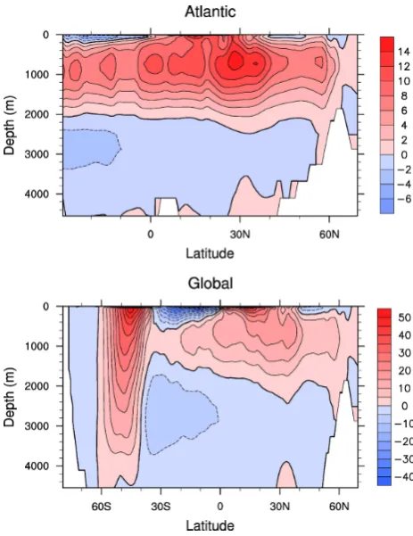
The maximum meridional overturning strength in the North Atlantic appears to be in line with observation-based estimates. Note, however, that only 60% of deep-water formed in the North Atlantic is exported to the Southern Ocean (Fig. 10). Accordingly, the Atlantic Ocean northward heat transport simulated by CCSM2/T31x3a is at the lower end of the range suggested by observations. In addition, the
Fig. 9. Monthly (blue) and annual-mean (red) transport time series
for the Antarctic Circumpolar Current at Drake Passage. Note that deep-ocean acceleration is applied from (surface) year 8 to (surface) year 300.
flow of NADW is relatively shallow and the total formation of AABW is weak (Fig. 10). For comparison: Ganachaud and Wunsch (2000) estimate a northward AABW flow of 5– 7 Sv into the Atlantic, 4–12 Sv into the Indian, and 5–9 Sv into the Pacific Ocean.
A rather unusual feature of CCSM2/T31x3a’s NADW overturning cell is the strong sinking around 40◦N in addi-tion to the common sinking branch around 60◦N (cf. Stouf-fer et al., 2006). A quite similar pattern is produced by CCSM3/T31 (cf. Yeager et al., 2006). Showing vertical ve-locities at 750 m depth in the North Atlantic, Fig. 11 provides some insight into the three-dimensional structure of the over-turning circulation. It is clearly visible that the mid-latitude sinking branch of the AMOC is associated with a wide area of downward motion along the path of the North Atlantic Current. It is unclear why other models show this behaviour only to a lesser extent or not at all. Surface heat fluxes and oceanic mixing processes are likely to play a role. However, extensive sensitivity studies were required to better define and resolve this problem.
receives water basically from the Pacific North Equatorial Current (cf. Gordon, 2001). The Atlantic Equatorial Under-current is mainly fed from the South Atlantic (South Equato-rial Current).
The Benguela Current, appearing below the Ekman layer, separates from the African coast far too south. Similar prob-lems arise with other eastern boundary currents (e.g. the Humboldt Current). Given the rather coarse resolution of the model grid, subtropical western boundary currents – includ-ing Kuroshio, Gulf Stream, East Australian Current, Mozam-bique Current, and Brazil Current – are simulated satisfacto-rily. As in reality, the Brazil Current is conspicuously weak as compared with the other western boundary currents (cf. Peterson and Stramma, 1991).
At high southern latitudes, the flow field is dominated by the ACC. South of the ACC, the westward flowing Antarc-tic Coastal Current is simulated. Around the southern tip of Africa, the model version of the Agulhas Current/leakage transports water from the Indian Ocean to the South Atlantic. This transport may be an integral part of the global conveyor belt circulation (Gordon, 1986). In the North Atlantic, a strong North Atlantic Current marks the boundary between the subtropical gyre and the cyclonic subpolar gyre. Pro-viding the convective regions south of Greenland and in the Nordic Seas with warm and salty water, the simulation of the North Atlantic Current is of utmost importance for the ther-mohaline circulation.
The flow field at 2000 m depth is characterized by a vigor-ous circulation around Antarctica. In the Atlantic Ocean, the southward movement of NADW constitutes the lower limb of the thermohaline overturning circulation. The NADW flow path forms an anticyclonic loop in the North Atlantic, which has no counterpart in observations. South of 30◦N,
the southward flow of NADW is confined to the Deep West-ern Boundary Current.
Potential temperatures simulated by CCSM2/T31x3a are shown in Fig. 13 along with observational data. Modelled sea surface temperatures (SST) in the tropical Indian and Pacific oceans are lower than observed. This cold bias is up to 2 K in the equatorial central Pacific (see also Fig. 28). The cold sur-face temperatures are associated with a larger than observed low-level cloud cover over the equatorial Pacific (not shown). In the tropical Atlantic, the western warm pool is too cold and the zonal SST gradient has the wrong sign. The tropical cold temperature bias is also visible at 100 m depth. The most pronounced deficiencies at subtropical latitudes are found in the eastern boundary currents and major upwelling re-gions (along the west coasts of North America, South Amer-ica, northwest AfrAmer-ica, and southwest Africa), where surface and subsurface temperatures are too warm. In northern high latitudes, the North Atlantic Current provides for moderate water temperatures south of Iceland and in the Norwegian Sea. Compared to the standard CCSM2/T31 control run (not shown), the model adjustments result in upper-ocean temper-atures in the northern North Atlantic that are much more in
Fig. 10. Mean Atlantic (top) and global (bottom) Eulerian
merid-ional overturning circulation (Sv). Positive values indicate clock-wise circulation. Since only the Eulerian portion of the circulation is shown, a spurious wind-driven overturning cell (so-called Dea-con cell) appears in the ACC region (Southern Ocean). As doc-umented by Danabasoglu et al. (1994), there is a substantial can-cellation between the Eulerian and bolus velocity terms in the La-grangian tracer velocity for the ACC region when using the Gent-McWilliams isopycnal scheme as in CCSM2/T31x3a (not shown here).
line with observations. At 500 m depth, the modelled Pacific, Indian and North Atlantic subtropical gyres exhibit higher temperatures compared to observations, whereas the subtrop-ical South Atlantic is slightly too cold in CCSM2/T31x3a. At 2000 m in the North Atlantic, simulated NADW has a po-tential temperature of about 4.5◦C. Deep temperatures in the Pacific and Indian oceans are∼1 K colder than in observa-tions, pointing to a cold bias in AABW. A similar deep-ocean cold bias has been found in a higher resolution version of the model (Kiehl and Gent, 2004).
Fig. 11. Annual-mean ocean vertical velocities (m/day) at 750 m depth in the North Atlantic (positive values indicate upward flow).
exhibits surface salinities which are now much closer to ob-servations. However, low-salinity water still caps off the Labrador Sea (cf. Fig. 28), forcing convection to occur fur-ther to the east. The reason for this shortcoming is unclear. Deficiencies in the wind stress curl, however, are likely to play a crucial role in the formation of the Labrador low-salinity cap (Gnanadesikan et al., 2006). In the Nordic Seas and northern North Atlantic, winter convection and, hence, deep-water formation takes place where upper-ocean salini-ties are around or above 35 psu.
In the South Atlantic, the model exhibits an upper-ocean fresh bias. The subtropical front is marked by the 34.9 psu isohaline at 100 m depth. In observations, the front resides well to the south of the Cape of Good Hope and the Aus-tralian continent. In CCSM2/T31x3a, the subtropical front is shifted far to the north (cf. Fig. 14). Part of this fresh bias can be attributed to excessive rainfall between 35◦S and 60◦S
(see Fig. 21). In the southeastern Atlantic, a possible source of error is the lack of Agulhas eddies that transport salty wa-ter into the Atlantic. A much finer grid resolution would be required to simulate the formation of these eddies.
Relatively high salinities are found in the North Pacific, whereas the upper Indian Ocean is overly fresh. In particular, the salinity of Australasian Mediterranean Water (AAMW) at the surface (at 100 m depth) is about 1 psu (0.5 psu) be-low observational values. At 500 m depth, the signature of AAMW is well captured by the model, still the region around Madagascar is too fresh. The salinity field at 2000 m reveals somewhat saltier NADW in the model compared to observa-tions. Traces of Eurafrican Mediterranean Water are absent at 2000 m depth in both the temperature (Fig. 13) and salinity (Fig. 14) fields of the model.
4.2.2 Sea ice
Maximum and minimum sea-ice conditions in the Northern and Southern Hemispheres simulated by CCSM2/T31x3a are displayed in Fig. 15. The use of optimized sea-ice/snow
4.2.3 Atmosphere
The overall performance of CCSM2/T31x3a with respect to the climatology of atmospheric basic surface variables (SLP, reference height air temperature, precipitation) is de-scribed in the following. Figure 16 displays the geograph-ical mean pattern of December–February (DJF) SLP simu-lated by the model against NCEP reanalysis data. The core positions of subpolar lows and subtropical highs are gener-ally well captured in CCSM2/T31x3a, although the centers of the Icelandic Low and Azores High are slightly displaced eastward relative to observations. The strengths of the sub-tropical highs are overestimated in the Northern Hemisphere, and underestimated in the Southern Hemisphere. Anoma-lously high pressure is found in Arctic and sub-Arctic re-gions, where the model produces too much sea ice and too cold surface air temperatures (Labrador Sea, Greenland Sea, Barents Sea). Over Canada, the simulated winter pressure is lower than observed by up to 9 hPa. In high southern lati-tudes, the model exhibits a low pressure-bias over the sub-polar seas, and a high-pressure bias over the Antarctic conti-nent.
During June–August (JJA) the simulated strengths of sub-tropical highs are close to reanalysis data in the South-ern Hemisphere (Fig. 17). In the Northern Hemisphere, CCSM2/T31x3a exhibits a pronounced high-pressure bias over the mid-latitude oceans. In the Arctic realm, the sim-ulated SLP is more than 6 hPa larger than in NCEP data with a maximum deviation over Greenland. Antarctic and sub-Antarctic regions in the model climate are characterized by a strong low-pressure bias relative to reanalysis data. A similar seasonality of the Antarctic SLP bias (high pressure during DJF, low pressure during JJA) has been found in other cli-mate models (e.g. Min et al., 2004). It should be noted, how-ever, that errors in the reanalysis data cannot be excluded for these extreme regions.
The deviation in simulated annual-mean SLP (Fig. 18) is associated with anomalously weak westerlies at the latitude of Drake Passage relative to NCEP data. The poor simula-tion of Southern Ocean wind forcing may partly be respon-sible for the low volume transport in the ACC (see above). Moreover, it may partly account for the model’s bias towards a weak AMOC (cf. McDermott, 1996; Gnanadesikan, 1999). The geographical pattern of DJF 2-meter air temperature over land is shown in Fig. 19. The winter surface climate of CCSM2/T31x3a is too warm over Greenland, northeast-ern Asia, and northnortheast-ern North America. The North American warm bias is associated with a low SLP anomaly (Fig. 16). During the summer season, simulated air temperatures are in better agreement with observations (Fig. 20). An overall cold bias for African and South American climates, however, is visible in both seasons. The same holds true for a pro-nounced warm bias over Antarctica.
A comparison of the simulated geographical distribution of annual-mean precipitation rate with CMAP observations
Fig. 12. Annual-mean ocean velocities at the surface (top), at 100 m
depth (middle), and at 2000 m depth (bottom).
Fig. 13. Annual-mean ocean temperature (◦C) at different depths simulated by CCSM2/T31x3a (left) and from Levitus data (right).
and northern South America, while the coastal areas of Peru and Ecuador are too wet. Over the tropical ocean, the dif-ference plot between model and data reveals several short-comings in the simulation: an east-west dipole over the In-dian Ocean, a north-south dipole over the equatorial Atlantic owing to a rather diffuse Atlantic Intertropical Convergence Zone (ITCZ) in the model annual average, and a “double
ITCZ” in the eastern Pacific. The “double ITCZ” emerges from a spurious zonal band of excess rainfall just south of the equator, whereas the observations reveal a maximum extend-ing from the west Pacific warm pool south-eastwards towards French Polynesia (the South Pacific Convergence Zone).
Fig. 14. Annual-mean ocean salinity (psu) at different depths simulated by CCSM2/T31x3a (left) and from Levitus data (right).
data. While the major meridional shift in observed tropi-cal precipitation from the southern to the Northern Hemi-sphere takes place from March to April, it occurs between May and July in the model. During that time, zonal-average CCSM2/T31x3a precipitation shows a false double structure of the ITCZ. In observations, the zonally averaged precipita-tion rate has a Northern Hemisphere maximum from June to August. In the model, the Northern Hemisphere maximum
Fig. 15. Sea-ice thickness during months of maximum (top) and minimum (bottom) ice cover for the Arctic (left) and Antarctic (right).
Numbers mark ice thicknesses based on observations (Strass and Fahrbach, 1998; Harms et al., 2001; Rothrock et al., 2003).
4.2.4 Total heat transport
Annual averaged meridional heat transports by the ocean, the atmosphere, and the coupled system are displayed in Fig. 23 and compared with NCEP-derived values. In CCSM2/T31x3a, the maximum meridional ocean heat trans-port is 1.3 PW in the Northern Hemisphere, and 1.2 PW in the Southern Hemisphere. These transports are about 0.5 PW
Fig. 16. December–February (DJF) mean sea-level pressure: CCSM2/T31x3a control run versus NCEP 1979–1998 reanalysis data (rmse =
Fig. 17. June–August (JJA) mean sea-level pressure: CCSM2/T31x3a control run versus NCEP 1979–1998 reanalysis data (rmse =
Fig. 18. Difference in annual-mean sea-level pressure between CCSM2/T31x3a and NCEP 1979–1998 reanalysis data (rmse =
root-mean-square error).
4.3 Climate variability 4.3.1 Tropical Pacific
Tropical climate variability on the short-range timescale from a few months to several years is dominated by the El Ni˜no/Southern Oscillation (ENSO). Figure 24 shows the wavelet power spectrum of the Ni˜no-3.4 index (SST 5◦S– 5◦N, 170◦W–120◦W) calculated from the synchronous
inte-gration phase of the CCSM2/T31x3a control run. The global wavelet power spectrum exhibits a maximum around 2 years, while the ENSO period deduced from observational data has a broader spectral peak near 3–7 years.
For a closer inspection of tropical Pacific variability, Fig. 25 displays Hovm¨oller plots of equatorial SST and 850-hPa zonal-wind anomalies. A 20-year interval has been cho-sen which includes two very strong El Ni˜no events (years 366/367 and 368/369) and a phase of reduced ENSO fre-quency (years 370–378). Comparing the SST anomalies with the 850-hPa zonal-wind anomalies reveals a strong atmosphere-ocean coupling in the model tropics. Wind anomalies are particularly pronounced during the two strong El Ni˜no events as well as during the two strong cold La Ni˜na events in years 365/366 and 370. Compared to observations, the amplitude of SST variations is too small in the model tropical Pacific. Moreover, CCSM2/T31x3a simulates the strongest SST fluctuations in the central part of the basin, while SST variability in the eastern Pacific is substantially underestimated. Likewise, maximum zonal-wind anomalies are situated too far in the west compared to observations.
It has been shown by Latif et al. (2001) and AchutaRao and Sperber (2002) that many climate models are not capable of simulating ENSO’s phase locking to the annual cycle. To test the skill of CCSM2/T31x3a in simulating the seasonal
cycle phase-locking, the interannual standard deviations of the Ni˜no-3.4 SST anomalies are calculated as a function of calendar month (Fig. 26). Although CCSM2/T31x3a sim-ulates a secondary maximum in August, the strongest vari-ability occurs during boreal winter. It is therefore concluded that, compared to other models, CCSM2/T31x3a shows rea-sonably good skill in simulating the seasonal cycle phase-locking.
4.3.2 North Atlantic
Fig. 19. December–February (DJF) reference height (2 m) air temperature: CCSM2/T31x3a control run versus Willmott/Matsuura 1950–
Fig. 21. Annual-mean precipitation rate: CCSM2/T31x3a control run versus Xie/Arkin (CMAP) 1979–1998 observations (rmse =
Fig. 22. Mean annual cycle of zonally averaged precipitation: CCSM2/T31x3a control run versus Xie/Arkin (CMAP) 1979–1998
observa-tions.
5 Discussion
5.1 Common biases
CCSM2/T31x3a produces an overall reasonable present-day global climate. Nevertheless, the evaluation of the control run has revealed several shortcomings. Most of these short-comings are well known as “typical problems” (i.e. com-mon biases) in global, non-flux-corrected climate models. A strong surface cold bias in the equatorial Pacific, a wrong
sign of the tropical Atlantic zonal SST gradient, and posi-tive SST biases at the eastern boundaries of the subtropical Pacific and Atlantic ocean basins (coastal upwelling regions of North/South America, northwestern/southwestern Africa) were to be expected from the history of ocean climate mod-elling (Mechoso et al., 1995; Latif et al., 2001; AchutaRao and Sperber, 2002; Davey et al., 2002; Wittenberg et al., 2006).
Fig. 23. Mean northward heat transports as derived from the CCSM2/T31x3a control run (left) and NCEP 1979–1998 reanalysis data (right)
for ocean, atmosphere, and the coupled system (TOA = Top of atmosphere). The heat transports are total and thus include all eddy transports.
Fig. 24. Wavelet (Morlet) power spectrum (Torrence and Compo, 1998) of the Ni˜no-3.4 index calculated from the CCSM2/T31x3a control
run (monthly values from the 100-yr synchronous integration phase): Temporal evolution (left), where the contour levels are chosen so that 75%, 50%, 25%, and 5% of the wavelet power (K2) is above each level (black contour is the 5% significance level, using a red-noise, autoregressive lag 1 background spectrum), and global wavelet power spectrum (right). The dotted curve marks the significance for the global wavelet spectrum.
clouds in the atmosphere model) and wind stress ocean forc-ing (drivforc-ing the coastal upwellforc-ing of cold thermocline wa-ter through surface Ekman divergence) each contribute about one-half to the common eastern boundary SST bias in global climate models (Kiehl and Gent, 2004; Large and Danaba-soglu, 2006). The representation of narrow coastal upwelling is also strongly dependent on the spatial resolution of the oceanic model grid. However, increasing the resolution of the ocean model does not necessarily reduce the SST
Fig. 25. Equatorial Pacific (5◦S–5◦N) monthly anomaly Hovm¨oller plots for SST (left) and 850-hPa zonal wind (right). A 20-yr interval from the synchronous CCSM2/T31x3a integration phase is shown (top) along with NCEP 1981–2000 data (bottom).
The rainfall double ITCZ is a common problem in coupled non-flux-corrected climate models (Mechoso et al., 1995; Lambert and Boer, 2001; Harvey, 2003; Covey et al., 2003; Li et al., 2004; Dai, 2006). A better simulation of the sur-face hydrography in the east Pacific coastal upwelling re-gions might improve the spatial structure of tropical rain-fall. Recently, Zhang and Wang (2006) demonstrated that the use of a modified Zhang-McFarlane convection scheme
J F M A M J J A S O N D 0.4
Month model
Fig. 26. Monthly standard deviations of the Ni˜no-3.4 SST index
calculated from the 100-yr synchronous CCSM2/T31x3a integra-tion phase (blue) and from 1950–2004 NCEP data (red).
biases over northeastern Asia and northern North America are often found in climate models (Lambert and Boer, 2001; Covey et al., 2003).
The movement and distribution of sea ice is strongly de-termined by the high-latitude wind field. Excessive ice build-up along the Siberian coast is mainly attributable to an erro-neous Arctic wind field and has been identified to be another common problem in many climate models (Bitz et al., 2002; DeWeaver and Bitz, 2006). Chapman and Walsh (2007) showed that, in the Barents Sea, nearly all state-of-the-art global climate models reveal a substantial oversimulation of sea ice associated with a strong cold bias in surface air tem-perature. Moreover, Chapman and Walsh (2007) pointed out that most models produce a positive SLP bias in the Eurasian sector of the Arctic Ocean.
The skill of models to simulate interannual variability in the tropical Pacific has been analysed in various studies. It has been found that most global climate models tend to produce ENSO-like variability that occurs at a higher-than-observed frequency (periodicity of 2–3 years instead of 3–7 years), and that most models are placing the maximum SST variability in the equatorial Pacific too far to the west (Latif et al., 2001; Davey et al., 2002; AchutaRao and Sperber, 2002). Although the latest climate models tend to be more realistic in representing the frequency with which ENSO occurs, and they are better at locating enhanced SST variability over the eastern Pacific (van Oldenborgh et al., 2005; AchutaRao and Sperber, 2006), CCSM2/T31x3a’s skill to simulate interan-nual variability in the tropical Pacific is well within the range of other models.
None of the above mentioned problems disappears in the higher-resolution (T42) version of CCSM2.0.1 or in
Fig. 27. Standard deviation of monthly mean 500-hPa geopo-tential height associated with the leading EOF corresponding to the NAO-like pattern in the North Atlantic region during four winter months (December–March) and percent variance explained: CCSM2/T31x3a synchronous integration phase (top) and NCEP re-analysis data (bottom).
Fig. 28. Annual-mean SST (top) and surface salinity (bottom) differences between CCSM control runs (CCSM2/T31x3a, left; CCSM3/T31,
right) and observations.
Table 3. Errors of mean values (first number) and root-mean-square errors (second number) with respect to global climatologies for different
versions of the Community Climate System Model (T31: low resolution; T42: medium resolution; T2m: 2-meter air temperature over land). The values for CCSM2/T42, CCSM3/T31 and CCSM3/T42 were taken from www.ccsm.ucar.edu/experiments and refer to the 1990 AD control runs b20.007 (average over years 561–580), b30.031 (average over years 801–820), and b30.004 (average over years 801–820), respectively.
Data set CCSM2/ CCSM2/ CCSM3/ CCSM3/ Units
T31x3a T42 T31 T42
NCEP SLP (DJF) +0.34, 3.84 +0.21, 3.62 −0.21, 3.91 −0.30, 3.17 hPa NCEP SLP (JJA) −0.38, 4.97 −0.47, 5.72 −0.97, 5.69 −1.00, 6.67 hPa Willmott T2m (DJF) +0.28, 4.12 +1.57, 4.70 −0.24, 3.70 +1.02, 3.93 K Willmott T2m (JJA) +0.16, 3.42 +1.11, 3.36 −1.04, 3.69 −0.26, 3.32 K CMAP Prec. (Ann.) +0.08, 1.19 +0.16, 1.24 +0.03, 1.28 +0.10, 1.38 mm/day
5.2 Potential side-effects of AMOC tuning
The tuning applied to CCSM2/T31x3a primarily aims at amplifying the AMOC. However, parameter changes might have substantial negative side-effects. In particular, Meehl et al. (2001) showed that larger values of vertical diffusiv-ity may reduce ENSO variance due to a lower sharpness of the tropical thermocline. Based on the results of uncou-pled ocean-only sensitivity experiments, it has also been sug-gested that the ACC volume transport through Drake Passage
decreases with increasing horizontal or isopycnal diffusivi-ties (Danabasoglu and McWilliams, 1995).
Fig. 29. Annual-mean salinity differences (psu) between CCSM control runs (CCSM2/T31x3a, left; CCSM3/T31, right) and observations
at 100 m depth in the North Atlantic.
years. Although the deep ocean has not reached equilibrium after this relatively short integration time, one can expect that both the volume transport of the ACC and the hydrography of the uppermost layers in the equatorial Pacific Ocean have largely been spun up.
Despite smaller horizontal mixing coefficients in the stan-dard CCSM2/T31 (cf. Sect. 2), the 10-year (years 278–287 of the control run) averaged ACC transport through Drake Passage is only 80.3 Sv, i.e. more than 10 Sv smaller than in CCSM3/T31x3a. Obviously, other (unknown) effects over-compensate for the influence of horizontal mixing on the ACC transport in the complex coupled system. Likewise, the effect of enhanced vertical mixing in CCSM2/T31x3a on ENSO variability is elusive. The standard deviation of an-nual mean Ni˜no-3.4 SST in the CCSM2/T31x3a control run is 0.36◦C, which is substantially smaller than the observa-tional value (ca. 0.64◦C for the period 1950–2005 AD). In the standard CCSM2/T31 control run, the standard deviation of annual mean Ni˜no-3.4 SST is 0.42◦C for the 10-year inter-val 278–287. Although the ENSO variance in CCSM2/T31 is slightly larger than in CCSM2/T31x3a (which was to be ex-pected as the background vertical mixing in the upper ocean is enhanced in CCSM2/T31x3a), this difference is not signif-icant at the 0.05 significance level according to an F-test. In summary, the negative side-effects of enhanced vertical mix-ing coefficients in CCSM2/T31x3a prove to be small or even negligible with respect to ACC and ENSO dynamics. 5.3 Comparisons with CCSM3/T31
Even though a detailed model intercomparison is far be-yond the scope of this paper, some examples shall be shown in which CCSM2/T31x3a provides a better simulation than CCSM3/T31. For this purpose, a present-day (1990 AD) control run with the standard CCSM3/T31 serves as a ref-erence (experiment b30.031; output data downloaded from
www.earthsystemgrid.org). Starting from observational data, CCSM3/T31 was synchronously integrated for 879 years. For the following comparisons with CCSM2/T31x3a, 80-year averages (80-years 800–879) from the CCSM3/T31 control run are used.
Figure 28 shows the global fields of SST and surface salin-ity errors from the CCSM2/T31x3a and CCSM3/T31 control runs. Both models are unable to produce the cold tempera-tures observed in coastal upwelling regions. In CCSM3/T31, a cold bias is particularly pronounced (>7◦C) in the North Pacific and North Atlantic oceans, where the SSTs in CCSM2/T31x3a are much closer to observations. As to surface salinity biases in CCSM3/T31 and CCSM2/T31x3a, the errors are quite comparable. The most obvious differ-ences are visible at high northern latitudes. In the northern North Pacific, CCSM2/T31x3a overestimates surface salin-ity, while CCSM3/T31 is too fresh. CCSM2/T31x3a’s sur-face salinities are also too high in the Arctic Ocean, where CCSM3/T31 tends to produce extremely fresh water masses. Both models simulate too fresh water in the northern North Atlantic. A zonal low-salinity tongue at around 40◦N, how-ever, is particularly troublesome in CCSM3/T31. This fresh bias is not restricted to the surface; it spoils the simulation also at subsurface levels (Fig. 29).
Fig. 30. Mean precipitation (m/yr) and near-surface winds (m/s) over West Africa for July–September as calculated from observa-tional/NCEP reanalysis data (top) and CCSM control runs (bottom). The land data for the precipitation climatology are based on histor-ical rain gauge measurements (Legates and Willmott, 1990), while oceanic precipitation is estimated from the Microwave Sounding Unit (Spencer, 1993).
flow penetrates as far north as 20◦N, where it converges with dry northerly winds at the monsoon trough. Both the wind and precipitation patterns are rather well captured by CCSM2/T31x3a. Most importantly, summer precipita-tion maxima reside on the African continent. By contrast, CCSM3/T31’s simulation of the summer low-level wind and precipitation fields over North Africa reveals several critical shortcomings. The northerly winds penetrate too far south, while the southerly monsoon flow is too weak (cf. Fig. 31). The most crucial problem in the CCSM3/T31 control run is the location of the tropical precipitation band. The model does not adequately simulate the summer migration of the rain belt onto the African continent. Instead, tropical precipi-tation maxima reside over the Guinea coast and over the Gulf of Guinea. It has been hypothesized that simulated warmer-than-observed SSTs in the Gulf of Guinea are responsible for excessive rainfall south of the Guinea coast (Meehl et al., 2006). The comparison between CCSM2/T31x3a and CCSM3/T31 corroborates this hypothesis, since the Gulf of
Guinea warm bias is much more pronounced in CCSM3/T31 than in CCSM2/T31x3a (cf. Fig. 28).
6 Conclusions
Fig. 31. Difference in July–September near-surface winds (m/s) between CCSM3/T31 and CCSM2/T31x3a over West Africa.
Mikolajewicz et al., 2007). Heat flux adjustment is not im-plemented either. The absence of air-sea heat flux adjustment avoids distortion in the non-linear dependence of heat fluxes on SST and sea ice.
In the present paper, important aspects of the present-day control run of CCSM2/T31x3a have been analysed, and ma-jor shortcomings have been exposed. Most biases found in the CCSM2/T31x3a control run have been identified as “typ-ical problems” in global climate modelling. Examples have been shown in which CCSM2/T31x3a has a better simu-lation skill than CCSM3/T31 (North Atlantic hydrography, West African monsoon). On the other hand, CCSM3/T31 has a stronger and more realistic ENSO SST variability in the tropical Pacific (cf. Yeager et al., 2006). There is also no doubt that for applications in which variations of the Arc-tic Ocean freshwater budget play a crucial role, special care should be taken with CCSM2/T31x3a due to the implemen-tation of the arctic/subarctic flux adjustment. Nevertheless, depending on the phenomenon under investigation and its geographical location, CCSM2/T31x3a is a useful alterna-tive to CCSM3/T31. Given its good simulation skills and its relatively low resource demands, CCSM2/T31x3a shows promise for studies of paleoclimate and other applications requiring long integrations and equilibrated solutions. Acknowledgements. The manuscript has benefited tremendously from comments and suggestions by Stephen Griffies. I would like to thank Michael Schulz and Ute Merkel for stimulating discussions and three anonymous reviewers as well as David Webb for their constructive comments. I am indebted to Manuel Renold and Christoph Raible for providing their POP analysis software. Thanks is due to Mark J. Stevens for making the CCSM Diagnos-tics Package available. The software package can be downloaded from www.cgd.ucar.edu/cms/stevens/master.html. The model run
AchutaRao, K. and Sperber, K. R.: ENSO simulation in coupled ocean-atmosphere models: are the current models better?, Clim. Dynam., 27, 1–15, 2006.
Alley, R. B. and Agustsdottir, A. M.: The 8k event: Cause and consequences of major Holocene abrupt climate change, Quat. Sci. Rev., 24, 1123–1149, 2005.
Bitz, C. M., Fyfe, J. C., and Flato, G. M.: Sea ice response to wind forcing from AMIP models, J. Climate, 15, 522–536, 2002. Bitz, C. M., Holland, M., Weaver, A. J., and Eby, M.: Simulating
the ice-thickness distribution in a coupled climate model, J. Geo-phys. Res., 106, 2441–2464, 2001.
Bitz, C. M. and Lipscomb, W. H.: An energy-conserving thermo-dynamic model of sea ice, J. Geophys. Res., 104, 15 669–15 677, 1999.
Bourke, R. H. and Garrett, R. P.: Sea ice thickness distribution in the Arctic Ocean, Cold Reg. Sci. Technol., 13, 259–280, 1987. Branstetter, M. L. and Erickson, D. J.: Continental runoff
dynamics in the Community Climate System Model (CCSM2) control simulation, J. Geophys. Res., 108, 4550, doi:10.1029/2003JD003212, 2003.
Briegleb, B. P., Bitz, C. M., Hunke, E. C., Lipscomb, W. H., and Schramm, J. L.: Description of the Community Climate System Model version 2: Sea ice model, Technical Report, Los Alamos National Laboratory, Los Alamos, New Mexico, National Center for Atmospheric Research, Boulder, Colorado, http://www.ccsm. ucar.edu/models/ccsm2.0.1/csim, 2002.
Broecker, W., Bond, G., Klas, M., Clark, E., and McManus, J.: Origin of the North Atlantic’s Heinrich events, Clim. Dynam., 6, 265–273, 1992.
Bryan, F.: Parameter sensitivity of primitive equation ocean general circulation models, J. Phys. Oceanogr., 17, 970–986, 1987. Bryan, K.: Accelerating the convergence to equilibrium in
ocean-climate models, J. Phys. Oceanogr., 14, 666–673, 1984. Bryan, K.: Efficient methods for finding the equilibrium climate of
coupled ocean-atmosphere models, in: Physically-based mod-elling and simulation of climate and climate change – Part I, edited by: Schlesinger, M. E., Kluwer Academic Publishers, 567–582, 1988.
Bryan, K. and Lewis, L. J.: A water mass model of the world ocean, J. Geophys. Res., 84, 2503–2517, 1979.
Canuto, C., Hussaini, M. Y., Quarteroni, A., and Zang, T. A.: Spec-tral methods in fluid dynamics, Springer-Verlag, Berlin, 567 pp., 1988.
Claussen, M., Mysak, L. A., Weaver, A. J., et al.: Earth system mod-els of intermediate complexity: Closing the gap in the spectrum of climate system models, Clim. Dynam., 18, 579–586, 2002. Collins, W. D., Hack, J. J., Boville, B. A., et al.: Description of the
NCAR Community Atmosphere Model (CAM2), Technical Re-port, National Center for Atmospheric Research, Boulder, Col-orado, http://www.ccsm.ucar.edu/models/atm-cam/docs/cam2.0/ description/index.html, 2003.
Covey, C., AchutaRao, K. M., Cubasch, U., et al.: An overview of results from the Coupled Model Intercomparison Project, Global Planet. Change, 37, 103–133, 2003.
Dai, A.: Precipitation characteristics in eighteen coupled climate models, J. Climate, 19, 4605–4630, 2006.
Danabasoglu, G.: A comparison of global ocean general circula-tion model solucircula-tions obtained with synchronous and accelerated integration methods, Ocean Model., 7, 323–341, 2004.
Danabasoglu, G. and McWilliams, J. C.: Sensitivity of the global ocean circulation to parameterizations of mesoscale tracer trans-ports, J. Climate, 8, 2967–2987, 1995.
Danabasoglu, G., McWilliams, J. C., and Gent, P. R.: The role of mesoscale tracer transports in the global ocean circulation, Sci-ence, 264, 1123–1126, 1994.
Danabasoglu, G., McWilliams, J. C., and Large, W. G.: Approach to equilibrium in accelerated global oceanic models, J. Climate, 9, 1092–1110, 1996.
Davey, M. K., Huddleston, M., Sperber, K. R., et al.: STOIC: a study of coupled model climatology and variability in tropical ocean regions, Clim. Dynam., 18, 403–420, 2002.
Deser, C., Capotondi, A., Saravanan, R., and Phillips, A. S.: Tropi-cal Pacific and Atlantic climate variability in CCSM3, J. Climate, 19, 2451–2481, 2006.
DeWeaver, E. and Bitz, C. M.: Atmospheric circulation and its ef-fect on Arctic sea ice in CCSM3 simulations at medium and high resolution, J. Climate, 19, 2415–2436, 2006.
Driscoll, N. W. and Haug, G. H.: A short circuit in the ocean’s ther-mohaline circulation: A cause for northern hemisphere glacia-tion?, Science, 282, 436–438, 1998.
Dukowicz, J. K. and Smith, R. D.: Implicit free-surface formulation of the Bryan-Cox-Semtner ocean model, J. Geophys. Res., 99, 7991–8014, 1994.
Folland, C. K., Palmer, T. N., and Parker, D. E.: Sahel rainfall and worldwide sea temperatures, Nature, 320, 602–607, 1986. Ganachaud, A. and Wunsch, C.: Improved estimates of global
ocean circulation, heat transport and mixing from hydrographic data, Nature, 408, 453–457, 2000.
Gent, P. R. and McWilliams, J. C.: Isopycnal mixing in ocean cir-culation models, J. Phys. Oceanogr., 20, 150–155, 1990. Gerdes, R. and Koeberle, C.: On the influence of DSOW in a
nu-merical model of the North-Atlantic general circulation, J. Phys. Oceanogr., 25, 2624–2642, 1995.
Giannini, A., Saravanan, R., and Chang, P.: Oceanic forcing of Sa-hel rainfall on interannual to interdecadal time scales, Science, 302, 1027–1030, 2003.
Gnanadesikan, A.: A simple predictive model for the structure of the oceanic pycnocline, Science, 283, 2077–2079, 1999. Gnanadesikan, A., Dixon, K. W., Griffies, S. M., et al.: GFDL’s
CM2 global coupled climate models. Part II: The baseline ocean simulation, J. Climate, 19, 675–697, 2006.
Gordon, A. L.: Inter-ocean exchange of thermocline water, J.
Geo-phys. Res., 91, 5037–5046, 1986.
Gordon, A. L.: Interocean exchange, in: Ocean circulation and cli-mate, edited by: Siedler, G., Church, J., and Gould, J., Academic Press, San Diego, 303–314, 2001.
Griffies, S. M.: The Gent-McWilliams skew-flux, J. Phys. Oceanogr., 28, 831–841, 1998.
Harms, S., Fahrbach, E., and Strass, V. H.: Sea ice transports in the Weddell Sea, J. Geophys. Res., 106, 9057–9074, 2001.
Harvey, L. D. D.: Characterizing and comparing the control-run variability of eight coupled AOGCMs and of observations. Part 2: precipitation, Clim. Dynam., 21, 647–658, 2003.
Hasumi, H.: Sensitivity of the global thermohaline circulation to interbasin freshwater transport by the atmosphere and the Bering Strait throughflow, J. Climate, 15, 2516–2526, 2002.
Haug, G. H. and Tiedemann, R.: Effect of the formation of the Isthmus of Panama on Atlantic Ocean thermohaline circulation, Nature, 393, 673–676, 1998.
Holland, M. M., Bitz, C. M., Hunke, E. C., Lipscomb, W. H., and Schramm, J. L.: Influence of the sea ice thickness distribution on polar climate in CCSM3, J. Climate, 19, 2398–2414, 2006. Huber, M. and Nof, D.: The ocean circulation in the Southern
Hemisphere and its climatic impacts in the Eocene, Palaeogeogr., Palaeoclimat., Palaeoecol., 231, 9–28, 2006.
Huber, M. and Sloan, L. C.: Heat transport, deep waters, and ther-mal gradients: Coupled simulation of an Eocene greenhouse cli-mate, Geophys. Res. Lett., 28, 3481–3484, 2001.
Hunke, E. C. and Dukowicz, J. K.: An elastic-viscous-plastic model for sea ice dynamics, J. Phys. Oceanogr., 27, 1849–1867, 1997. Jongma, J. I., Prange, M., Renssen, H., and Schulz, M.:
Amplifica-tion of Holocene multicentennial climate forcing by mode tran-sitions in North Atlantic overturning circulation, Geophys. Res. Lett., 34, L15706, doi:10.1029/2007GL030642, 2007.
Kantha, L. H. and Clayson, C. A.: Numerical models of oceans and oceanic processes, Academic Press, 940 pp., 2000.
Kiehl, J. T. and Gent, P. R.: The Community Climate System Model, version 2, J. Climate, 17, 3666–3682, 2004.
Koesters, F., Kaese, R., Fleming, K., and Wolf, D.: Denmark Strait overflow for Last Glacial Maximum to Holocene conditions, Pa-leoceanogr., 19, PA2019, doi:10.1029/2003PA000972, 2004. Lamb, P. J.: Case studies of tropical Atlantic surface circulation
patterns during recent sub-saharan weather anomalies: 1967 and 1968, Mon. Weather Rev., 106, 482–491, 1978.
Lambert, S. J. and Boer, G. J.: CMIP1 evaluation and intercom-parison of coupled climate models, Clim. Dynam., 17, 83–106, 2001.
Large, W. G. and Danabasoglu, G.: Attribution and impacts of upper-ocean biases in CCSM3, J. Climate, 19, 2325–2346, 2006. Large, W. G., McWilliams, J. C., and Doney, S. C.: Oceanic vertical mixing: A review and a model with a nonlocal boundary layer parameterization, Rev. Geophys., 32, 363–403, 1994.
Latif, M., Sperber, K., Arblaster, J., et al.: ENSIP: the El Ni˜no simulation intercomparison project, Clim. Dynam., 18, 255–276, 2001.
Laxon, S., Peacock, N., and Smith, D.: High interannual variability of sea ice thickness in the Arctic region, Nature, 425, 947–950, 2003.
Meehl, G. A., Arblaster, J. M., Lawrence, D. M., Seth, A., Schnei-der, E. K., Kirtman, B. P., and Min, D.: Monsoon regimes in the CCSM3, J. Climate, 19, 2482–2495, 2006.
Meehl, G. A., Gent, P. R., Arblaster, J. M., Otto-Bliesner, B. L., Brady, E. C., and Craig, A.: Factors that affect the amplitude of El Ni˜no in global coupled climate models, Clim. Dynam., 17, 515–526, 2001.
Meehl, G. A., Stocker, T. F., Collins, W. D., et al.: Global cli-mate projections, in: Clicli-mate Change 2007: The physical science basis (Contribution of Working Group I to the Fourth Assess-ment Report of the IntergovernAssess-mental Panel on Climate Change), edited by: Solomon, S., et al., Cambridge University Press, Cam-bridge, 747–845, 2007.
Mikolajewicz, U., Groeger, M., Maier-Reimer, E., Schurgers, G., Vizcaino, M., and Winguth, A. M. E.: Long-term effects of an-thropogenic CO2 emissions simulated with a complex earth sys-tem model, Clim. Dynam., 28, 599–633, 2007.
Min, S.-K., Legutke, S., Hense, A., and Kwon, W.-T.: Climatology and internal variability in a 1000-year control simulation with the coupled climate model ECHO-G, M&D Technical Report, No. 2, Max Planck Institute for Meteorology, Hamburg, Germany, 67 pp., 2004.
Oppo, D. W., McManus, J. F., and Cullen, J. L.: Deepwater vari-ability in the Holocene epoch, Nature, 422, 277–278, 2003. Peltier, W. R. and Solheim, L. P.: The climate of the Earth at Last
Glacial Maximum: statistical equilibrium state and a mode of internal variability, Quat. Sci. Rev., 23, 335–357, 2004. Peterson, R. G. and Stramma, L.: Upper-level circulation in the
South Atlantic, Prog. Oceanogr., 26, 1–73, 1991.
Piotrowski, A. M., Goldstein, S. L., Hemming, S. R., and Fairbanks, R. G.: Temporal relationship of carbon cycling and ocean circu-lation at glacial boundaries, Science, 307, 1933–1938, 2005. Prange, M.: Influence of Arctic freshwater sources on the
circu-lation in the Arctic Mediterranean and the North Atlantic in a prognostic ocean/sea-ice model, Reports on Polar and Marine Research, No. 468, Alfred Wegener Institute, Bremerhaven, Ger-many, 220 pp., 2003.
Prange, M. and Gerdes, R.: The role of surface freshwater flux boundary conditions in Arctic Ocean modelling, Ocean Model., 13, 25–43, 2006.
Prange, M., Lohmann, G., and Paul, A.: Influence of vertical mixing on the thermohaline hysteresis: Analyses of an OGCM, J. Phys. Oceanogr., 33, 1707–1721, 2003.
Prange, M., Lohmann, G., Romanova, V., and Butzin, M.: Mod-elling tempo-spatial signatures of Heinrich Events: Influence
http://www.clim-past.net/3/97/2007/.
Seo, H., Jochum, M., Murtugudde, R., and Miller, A. J.: Ef-fect of ocean mesoscale variability on the mean state of tropical Atlantic climate, Geophys. Res. Lett., 33, L09606, doi:10.1029/2005GL025651, 2006.
Severinghaus, J. P. and Brook, E. J.: Abrupt climate change at the end of the last glacial period inferred from trapped air in polar ice, Science, 286, 930–934, 1999.
Smith, R. and Gent, P.: Reference manual for the Parallel Ocean Program (POP), Technical Report, Los Alamos National Lab-oratory, Los Alamos, New Mexico, National Center for Atmo-spheric Research, Boulder, Colorado, http://www.ccsm.ucar.edu/ models/ccsm2.0.1/pop, 2002.
Smith, R. D. and McWilliams, J. C.: Anisotropic horizontal viscos-ity for ocean models, Ocean Model., 5, 129–156, 2003. Spencer, R. W.: Global oceanic precipitation from the MSU during
1979–91 and comparisons to other climatologies, J. Climate, 6, 1301–1326, 1993.
Stammer, D., Wunsch, C., Giering, R., et al.: Volume, heat, and freshwater transports of the global ocean circulation 1993–2000 estimated from a general circulation model constrained by World Ocean Circulation Experiment (WOCE) data, J. Geophys. Res., 108, 3007, doi:10.1029/2001JC001115, 2003.
Steele, M., Morley, R., and Ermold, W.: PHC: a global ocean hydrography with a high quality Arctic Ocean, J. Climate, 14, 2079–2087, 2001.
Stouffer, R. J., Dixon, K. W., Spelman, M. J., et al.: Investigating the causes of the response of the thermohaline circulation to past and future climate changes, J. Climate, 19, 1365–1387, 2006. Strass, V. H. and Fahrbach, E.: Temporal and regional variation of
sea ice draft and coverage in the Weddell Sea obtained from up-ward looking sonars, in: Antarctic sea ice – Physical processes, interactions, and variability, edited by: Jeffries, M. O., Antarc-tic Res. Ser., 74, American Geophys. Union, Washington D.C., 123–139, 1998.
Torrence, C. and Compo, G. P.: A practical guide to wavelet analy-sis, B. Am. Meteorol. Soc., 79, 61–78, 1998.
van Oldenborgh, G. J., Philip, S. Y., and Collins, M.: El Ni˜no in a changing climate: a multi-model study, Ocean Sci., 1, 81–95, 2005,
http://www.ocean-sci.net/1/81/2005/.
Voelker, A. H. L. and workshop participants: Global distribution of centennial-scale records for marine isotope stage (MIS) 3: a database, Quat. Sci. Rev., 21, 1185–1214, 2002.
Wadley, M. R. and Bigg, G. R.: Impact of flow through the Cana-dian Archipelago on the North Atlantic and Arctic thermohaline circulation: an ocean modelling study, Q. J. Roy. Meteor. Soc., 128, 2187–2203, 2002.
Wang, D.: A note on using the accelerated convergence method in climate models, Tellus A, 53, 27–34, 2001.
Webb, D. J. and de Cuevas, B. A.: On the fast response of the South-ern Ocean to changes in the zonal wind, Ocean Sci., 3, 417–427, 2007,
http://www.ocean-sci.net/3/417/2007/.
Wittenberg, A. T., Rosati, A., Lau, N.-C., and Ploshay, J. J.: GFDL’s CM2 global coupled climate models. Part III: Tropical Pacific climate and ENSO, J. Climate, 19, 698–722, 2006.
Wright, D. G. and Stocker, T. F.: Sensitivities of a zonally averaged global ocean circulation model, J. Geophys. Res., 97, 12 707– 12 730, 1992.
Yeager, S. G., Shields, C. A., Large, W. G., and Hack, J. J.: The low-resolution CCSM3, J. Climate, 19, 2545–2566, 2006. Zhang, G. J. and Wang, H.: Toward mitigating the double ITCZ