www.ocean-sci.net/7/835/2011/ doi:10.5194/os-7-835-2011
© Author(s) 2011. CC Attribution 3.0 License.
Ocean Science
Extraction of spatial-temporal rules from mesoscale eddies
in the South China Sea based on rough set theory
Y. Du1, X. Fan1, Z. He2, F. Su1, C. Zhou1, H. Mao2, and D. Wang2
1State Key Laboratory of Resources and Environmental Information System, Institute of Geographic Science and Natural Resources Research, Chinese Academy of Sciences, Beijing, 100101, China
2Key Laboratory of Tropical Marine Environmental Dynamics, South China Sea Institute of Oceanology, Chinese Academy of Sciences, Guangzhou, 510301, China
Received: 29 March 2011 – Published in Ocean Sci. Discuss.: 14 June 2011
Revised: 14 October 2011 – Accepted: 26 October 2011 – Published: 7 December 2011
Abstract. In this paper, a rough set theory is introduced to
represent spatial-temporal relationships and extract the cor-responding rules from typical mesoscale-eddy states in the South China Sea (SCS). Three decision attributes are adopted in this study, which make the approach flexible in retriev-ing spatial-temporal rules with different features. The results demonstrate that this approach is effective, and therefore pro-vides a powerful approach to forecasts in the future studies. Spatial-temporal rules in the SCS indicate that warm eddies following the rules are generally in the southeastern and cen-tral SCS around 2000 m isobaths in winter. Their intensity and vorticity are weaker than those of cold eddies. They usu-ally move a shorter distance. By contrast, cold eddies are in 2000 m and deeper regions of the southwestern and north-eastern SCS in spring and fall. Their intensity and vorticity are strong. Usually they move a long distance. In winter, a few rules are followed by cold eddies in the northern tip of the basin and southwest of Taiwan Island rather than warm eddies, indicating cold eddies may be well-regulated in the region. Several warm-eddy rules are achieved west of Lu-zon Island, indicating warm eddies may be well-regulated in the region as well. Otherwise, warm and cold eddies are distributed not only in the jet flow off southern Vietnam in-duced by intraseasonal wind stress in summer-fall, but also in the northern shallow water, which should be a focus of a future study.
Correspondence to: C. Zhou ([email protected])
1 Introduction
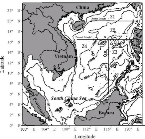
The South China Sea (SCS: 2◦300–23◦300N, 99◦100– 121◦500E) is the largest semi-enclosed marginal sea in the northwestern Pacific Ocean, as shown in Fig. 1. It has a large NE-SW oriented abyssal basin with greatest depth of 5567 m. There is an approximate 3.5×10⁶km2of total area with mean depth of 1212 m. The SCS is well linked to the adjacent seas through several straits or channels, connecting to the Pacific Ocean through the Luzon Strait, to the Sulu Sea through the Mindoro Strait, to the East China Sea through the Taiwan Strait and to the Java Sea through the Karimata Strait and so on.
Fig.1 Topography of the SCS.
(Z1: northeastern SCS; Z2: central SCS; Z3: southeastern SCS; Z4: southwestern SCS;
Solid lines are the boundaries of Z1, Z2, Z3 and Z4).
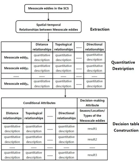
Fig.2 Flowchart of the procedure for representing spatial-temporal relationships among mesoscale eddy states
1
Fig. 1. Topography of the SCS. (Z1: northeastern SCS; Z2: central SCS; Z3: southeastern SCS; Z4: southwestern SCS; solid lines are the boundaries of Z1, Z2, Z3and Z4).
barotropic response to intraseasonal wind stress forcing in shallow water, and barotropic and baroclinic instabilities and eddy energy advection in deep water, with an exception off-shore from Vietnam in summer.
On the other hand, mesoscale variability also has an in-terannual variation as a response to El Nino/Southern Os-cillation (ENSO) in the SCS. Xiu et al. (2010) reveal that mesoscale eddy activities are not induced by the ENSO events directly, although interannual variabilities in SSH fields are highly correlated with ENSO (Xie et al., 2003; Liu et al., 2004; Wu and Chang, 2005; Fang et al., 2006; Wang et al., 2006). Previous works reveal that eddies are shed from strong currents such as the Gulf Stream and Kuroshio (Hurl-burt and Thompson, 1980; Li et al., 1998; Hetland et al., 1999), and then generate prominent spatial-temporal vari-ability in regional hydrography (Wu and Chiang, 2007). Ob-servational results show that, in winter, there is an anticy-clonic eddy shed from the Kuroshio loop due to an unstable Kuroshio meander in the northern Luzon Strait (Li and Wu, 1989; Jia and Liu, 2004); the eddy subsequently moves west-ward into the SCS (Li et al., 1998; Wang et al., 2000; Yuan et al., 2006). Direct views of eddy-shedding events can be provided by satellite remote sensing data (Yuan et al., 2007; Li, 2002; Su et al., 2002). Numerical studies also support this notion (Yang et al., 2000; Metzger and Hurlburt, 2001) and discuss eddy-shedding mechanisms (Jia et al., 2005). The previous studies reveal that mesoscale eddies propagate westward with a speed of 0.1 m s−1, the order of magnitude of the phase speed of baroclinic Rossby waves in the SCS (e.g. Wu et al., 2005; Wu and Chiang, 2007; Hwang et al.,
2004; Roemmich and Gilson, 2001; Hu et al., 2001; White, 2000; D. Wang et al., 2008). Topographic eddies can be in-duced by an eddy-shedding process resulting from the inter-action between unstable rotating fluid and sharp topography in the SCS (Yuan and Wang, 1986; Hu et al., 2001).
Among methods of studying eddies, cruise observation is difficult and expensive, so that only sparse data can be achieved. Numerical modeling depends heavily on specific boundary conditions and also intensive computation. Re-mote sensing is good at extracting instantaneous state rather than continuous evolution of mesoscale eddies. Therefore, it is necessary to introduce a new approach to extract spatial-temporal rules from eddies efficiently in order to depict their distribution pattern in-depth and quantitatively.
Rough set theory is an approach to extract and represent the knowledge that can be derived from incomplete datasets with uncertainties (Miao and Li, 2008). Since rough set theory is available to analyze data with insufficient and in-complete knowledge, it has been applied in many traditional domains, including finance, medicine, telecommunications, vibration analysis, control theory, signal analysis, pattern recognition, and image analysis (Yasdi, 1996; Polkowski and Skowron, 1998; Polkowski et al., 2000; Skowron, 2001; Le-ung and Li, 2003). In this paper, rough set theory is in-troduced to extract spatial-temporal rules from mesoscale eddies during November 2003–June 2009 in the SCS. In Sect. 2, we present the rough set theory and spatial-temporal relationships representation. Data sources and the spatial-temporal rules of mesoscale eddies in the SCS are described in Sect. 3. The findings are discussed in Sect. 4, followed by a conclusion in Sect. 5.
2 Data and method
2.1 Data
Raw data can be acquired from output of the US Naval Re-search Laboratory (NRL, http://www7320.nrlssc.navy.mil/ global nlom32/scs.html) the NRL Layered Global Ocean Model (NLOM), including SSH, SST (Sea surface tempera-ture) and surface current speed. The SSH data is assimilated from satellite data acquired by ENVISAT, GFO and JASON-1, etc. The SST data is assimilated from IR data with a tem-poral resolution of 1 day and a horizontal spatial resolution of (1/32)◦×(1/32)◦. The SCS is divided into 4 zones (Z1– Z4, shown in Fig. 1), according to generating mechanisms of mesoscale eddies (Wang, 2004). We identify eddies in the SCS and track their evolution process from 5-yr-and-8-month time series of SSH data during November 2003–June 2009 in accordance with the following four criteria:
2. The horizontal scale is not less than 100 km (Wang et al., 2003; Lin et al., 2007).
3. The eddy can be tracked over 20 days.
4. The SSH difference between center of an eddy and its outmost contour, intensity of an eddyM, is not less than 8 cm (Lin et al., 2007).
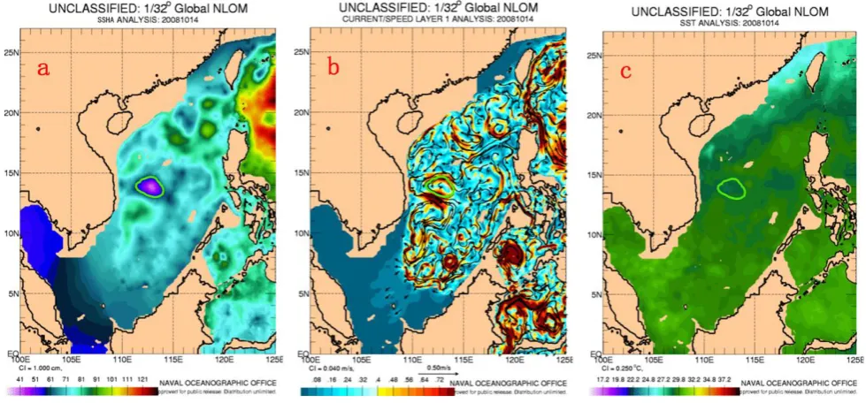
Wang et al. (2003) choose 30 days as the minimal lifetime of eddy processes, and Lin et al. (2007) choose 5 weeks. In this paper, shorter-lifetime eddies are able to be detected, owing to highly-resolved data. Eddy state is defined as a “time-slice” of an eddy process at one moment. In total, 391 typ-ical mesoscale-eddy states, including 291 warm-eddy states and 100 cold-eddy states, are detected in this paper. Gener-ally, one image represents one state, rather than more than one image represents one state. One of them with the corre-sponding modeling image is illustrated in Fig. 4a–c.
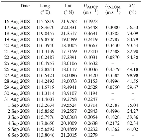
Initially, reliability of the modeling performance needs to be evaluated by comparing with hydrographic observa-tion. SSHA (Sea surface height anomaly) was obtained from NLOM SSH fields during 2003–2009. AVISO merged tem-poral 7-day and spatial (1/12)◦×(1/12)◦sea level anomaly (SLA) observation is adopted to check the accuracy of NLOM SSHA. In Fig. 5a–e, several deterministic eddies of the SCS are shown, e.g. a warm eddy off the Luzon Strait (marked as red capital A), the eddy pair offshore from Viet-nam (red capital D), in summer-fall, and its process of evo-lution are well reflected in NLOM SSHA. The warm eddy near Paracel Island (red capital C) and the west Luzon eddy (Qu, 2000; red capital B) are also well-reflected in the north-ern SCS. In addition, a cruise measurement was performed during 16 August–6 September 2008. Hourly current veloc-ity was gathered by using ADCP (supported by South China Sea Institute of Oceanology, Chinese Academy of Sciences, China). Near-sea surface current speeds (38 m beneath) were selected to validate those at the corresponding positions sim-ulated by NLOM. Comparison of the current speeds simu-lated by NLOM with cruise measurements is shown in Ta-ble 1. Accuracy of current speed is calculated as
δU=
1−
UNLOM−UADCP
UADCP
·100% (1)
where UNLOM is the surface current speed simulated by NLOM.UADCPis the 38 m-layer current speed recorded by ADCP. δU is the ratio of accuracy. δU at 8 (out of 15) stations exceeds 70 %. Therefore, we consider the NLOM SSHA acceptable in the SCS.
2.2 Rough set theory
Rough set is a mathematical approach proposed by Pawlak (1982) to extract decision rules from a decision sys-tem, which is a special case of an information system. For-mally, a decision system can be represented by the form
Table 1. Comparison of current speed derived from NLOM with
cruise measurement.
Date Long. Lat. UADCP UNLOM δU (◦E) (◦N) (m s−1) (m s−1) (%)
16 Aug 2008 115.5819 21.9792 0.1972 – – 17 Aug 2008 118.4670 22.0331 0.5448 0.3080 56.53 18 Aug 2008 119.8457 21.3517 0.4631 0.3385 73.09 19 Aug 2008 119.8736 19.0399 0.2419 0.2787 84.79 20 Aug 2008 116.3940 18.1005 0.3667 0.3430 93.54 21 Aug 2008 111.3139 17.3159 0.2210 0.2588 82.90 22 Aug 2008 110.2487 17.3391 0.1031 0.0870 84.38 25 Aug 2008 110.4957 18.0106 0.1632 – – 26 Aug 2008 112.8241 18.0117 0.3036 0.4579 49.18 27 Aug 2008 116.5421 18.0086 0.3420 0.3385 98.98 28 Aug 2008 114.2493 18.0073 0.3153 0.4996 41.55 29 Aug 2008 111.5718 18.4941 0.2528 0.0750 29.67 30 Aug 2008 111.3114 18.9107 0.1194 – – 31 Aug 2008 111.4607 19.2758 0.2247 – – 1 Sep 2008 113.2634 19.5524 0.3714 0.2787 75.04 2 Sep 2008 115.8565 19.2557 0.2843 0.4996 24.27 3 Sep 2008 115.7976 20.0368 0.3054 0.1828 59.86 4 Sep 2008 117.0650 20.1009 0.2638 0.2172 82.34 5 Sep 2008 115.6592 20.4859 0.2232 0.1362 61.02 6 Sep 2008 113.8046 21.2015 0.1279 – –
S=(U,C∪D), whereU is a nonempty finite set of objects called the universe,C is a nonempty finite set of attributes, andD /∈C is the decision attribute. The elements ofC are condition attributes or simply conditions. The decision at-tributes may take several values, though binary outcomes are rather frequent (Komorowski et al., 1999). In this study, the universeU may be the whole set of mesoscale-eddy cases in the SCS, and the decision attribute D can be the place of origin, generating season or the type of mesoscale ed-dies. For example, we can associate the number 1 with a warm eddy, 0 with a cold eddy. Condition attributes inCare the factors associated with spatial-temporal characteristics of mesoscale eddies, such as intensity, the place of origin, hor-izontal scale and relationships between a target eddy and its reference eddy1.
2.2.1 Attribute reducts
Rough set analysis aims at synthesizing an approximation of concepts from acquired data (Bai et al., 2010). There are some concepts that cannot be fully defined in a crisp manner by attributes at hand, e.g. mesoscale ocean eddies cannot be classified by their hydrographic features. Rough sets use up-per and lower approximations to describe the uncertain con-cept.
1Reference eddy is defined as the nearest eddy to target eddy
In rough set theory, attribute reducts is a key step. The ba-sic idea is a classification (of the eddies inU) on the basis of attributes, using only attributes (inC) that help to refine the classification. We redundant attributes that do not distinguish between eddies in any “equivalence” class (i.e. eddies that are indistinguishable using all the retained attributes). There are usually several such subsets of attributes, and those that are minimal are called reducts (Komorowski et al., 1999).
The decision attribute D induces a partition of the uni-verse of objects U. Without any loss of generality, it is as-sumed thatVD (decision values) is the set of n partitioning
results according to the values of a geographical attribute
D{v1(D),...,vn(D)}, where vi(D) is said to be one of the
partitioning results. The induced partition is therefore the collection of equivalence classes Xv1(D),...,Xvn(D), called decision classes, where two objects are said to belong to the same decision class if they have the same result for the deci-sion attribute:Xi= {x∈U|D(x)=vi(D)}.
It is possible that two objects that are indistinguishable with respect to attributes C may belong to different decision classes. The decision system S is said to be inconsistent with respect to C if this is the case and consistent otherwise.
The decision table is then simplified using the algorithm proposed by Pawlak (1991), which is briefly summarized as follows. The positive region of D with respect to C, POSC(D)is given by
POSC(D)=
[
X∈U/D
CX (2)
where POSC(D)is a collection of all elements in U, which
can be uniquely categorized into an equivalence class of D by the partitioning U according to values of attribute C.Xis any member of U/D and U/D represents an equivalence class of the decision attributes.CXdenotes the lower approximation of X with respect to C, which meansX cannot be exactly represented because it may include some objects which are indistinguishable based on the attributesC.
CX= {x|[x]C⊆X}. (3)
Where [x]C denote the equivalence class of the C-indiscernibility relations, which can also be denoted as IND(C)for simplicity, means that if(x,x0)∈IND(C), then objectsxandx0reindiscernible from each other by attributes from C.
For an indexcin set C (∀c∈C.), if
POSC(D)=POSC−{c}(D) (4)
thencis dispensable in C with respect to D. Otherwise,cis indispensable in C with respect to D. If indices in C are all indispensable with respect to D, then C is totally indepen-dent with respect to D. Attribute reducts is a process to find a subset of C, which is totally indispensable with respect to D.
2.2.2 Decision rule extraction
Once the reducts are found, the rules are easily constructed by overlaying the reducts over the originating decision table and reading off the values. Let Xiand Yj be the equivalence
classes of U/C and U/D, respectively. des(Xi)represents the
description of equivalence class Xi, that is, the specific
val-ues of the condition attributes in set C. des(Yj)refers to the
description of equivalence class Yj, that is, the specific
val-ues of decision attributes in D. Decision rules then can be generated and expressed as
rij:des(Xi)→des(Yj) Yj∩Xi6=ø (5)
Both the certainty and coverage factors for each specific rule are calculated to determine whether the rule is essential or not (Pawlak, 2001). The certainty factor measures how likely the result (derived from a specific rule) is correct. The certainty factor is the proportion of instances in the database following both the condition attributes and the equivalence class of the decision attribute. For example, it means for the same region of the condition attribute space, how many of the instances in the database lead to the same class in the decision attribute. It can be given by
α=Xi∩Yj
/|Xi| 0< α <1 (6)
A high value of α. for a specific rule indicates that, if the condition attributes satisfy the rules, the decision results are more likely to be correct.
The coverage factor is defined as β=Xi∩Yj
/
Yj
0< β <1 (7)
which represents, to some extent, the condition attributes sat-isfying the rules for a specific result. The value 1 indicates that, for any result, the condition attributes completely sat-isfy the rules. The lower the value, the lower probability the attributes may observe the rules. The certainty and coverage factors are then calculated for all rules which were gener-ated from the reducts of set C. Only those rules (thereby the corresponding spatial relations) with certainty and coverage factors greater than a preset threshold are accepted.
Fig. 2. Flowchart of the procedure for representing spatial-temporal
relationships among mesoscale eddy states.
2.2.3 Application of rough set theory to mesoscale ocean eddies
Considering rough set theory does not need prior information in analyzing data; it can derive a classification or decision rules according to the knowledge reducts procedure. Hence, rough set theory can mine the objective and inherent rules implicit in the data. Given that the dynamic mechanisms of mesoscale eddies are still not grasped completely, our study adapts rough set theory to extract spatial distribution regular-ities of ocean eddies from highly-resolved ocean modeling data in quantity.
The whole process to extract spatial-temporal rules from mesoscale eddies by using rough sets can be divided into three steps (Fig. 2): (1) construct a decision information system based on the data at hand; (2) find minimal reducts of condition attributes; (3) generate rules according to the reducts.
In the first step, spatial-temporal relationship indices should be transformed from original data, which are then imported into the decision table. This step is crucial when rough set theory is used in spatial analysis of eddies. Many spatial attributes are continuous variables. Under such cir-cumstances, the continuous attributes should be discretized before performing rough set analysis. In our study, a boolean algorithm was chosen to discretize the continuous attributes. A Boolean reasoning algorithm was first proposed by Nguyen and Skowron (1995). The algorithm operates by first creating a Boolean function from the set of candidate cuts, which can be the sets of mean value of any two different values in numerical attributes, and then computing a prime implicant of the function. A prime implicant of the func-tion is an implicant that cannot be covered by a more general (more reduced – meaning with fewer literals). The subset of candidate cuts found by Boolean reasoning is a minimal set
Fig. 3. Flowchart of major analysis steps based on the rough set
theory.
of candidate cuts that preserves all discernibility inherent in the decision system (Skowron, 1995). It is used to discre-tise the decision table and a genetic algorithm is then applied to simplify and extract decision rules from relations between eddy attributes (Qhrn, 1999).
In the next step, as is described in Sect. 2.1, finding reducts is used as the attribute selection method. Not all attributes transformed or collected in the first step are the key factors that are related to the decision attribute. So it is important to select attributes that are in close relation to the decision.
Finally, spatial-temporal relationship rules of eddies in the SCS are generated from the reducts by overlaying the reducts over the originating decision table and reading off the values. The certainty and coverage factors of each specific rule are then calculated (Wang, 2001).
We present the detailed procedures to represent spatial-temporal relationships of mesoscale eddies, in view of the importance of the first step. As illustrated in Fig. 3, the pro-cedures as follows:
Fig. 4. Sketch map of a mesoscale eddy in the SCS (outlined by bright green contour).
2. These relationships are then described by a series of quantitative indices. For example, the RCC-8 model (Randell et al., 1992; Randell and Cohn, 1989) can be used to describe the topological relationship among eddies. The topological relations record the relation-ships in space such as connectivity, intersection and ad-jacency among objects.
3. Decision tables are constructed with each row repre-senting a case of an eddy, while columns record con-dition and decision attributes. The values in each row, except for the decision attributes, are the quantitative in-dices which are derived from spatial-temporal relation-ships.
According to the previous studies, two types of attributes of eddies are considered in this paper. One is their own char-acteristic attributes; another is features of spatial-temporal relationships. In total the attributes including:
1. Place of origin (Zone). According to generating mech-anisms of mesoscale eddies, the SCS is divided into 4 zones: northeastern, central, southeastern, and south-western zones (Wang, 2004), as shown in Fig. 1. 2. Generating season (Time). Spring is from March to
May, summer from June to August, fall from Septem-ber to NovemSeptem-ber, and winter from DecemSeptem-ber to next February.
3. Type of eddy (Type): warm or cold eddy.
4. Intensity of eddyM(Intensity): SSH difference in me-tres between the center and the periphery of an eddy.
5. Vorticity (Vorticity) with an approximation of the rela-tive vorticity of a eddy:
ς=∂v
∂x−
∂u
∂y≈
8gM
f D2 (8)
whereςis eddy’s vorticity in s−1,Meddy’s intensity,D eddy’s diameter. The Coriolis parameterf is 10−4s−1, and the acceleration of gravitygis 9.80 ms−2.
6. Horizontal scale of the eddy (HorizontalScale) in me-tres: the average of the major axis and the minor axis of an enclosing ellipse.
7. Temperature at the center of an eddy (CentralTemp) in Celsius degree.
8. Difference of temperature between the center and the periphery of an eddy (TempDiff) in Celsius degree. 9. Mean depth (Depth) in metres: the mean water depth at
the center of an eddy.
10. The Euclidean distance (Distance) in metres from the geometric center of a target eddy to its reference eddy. 11. Directional relationship (Direction) to the reference
Table 2. Decision table constructed from spatial-temporal relationships of mesoscale-eddy states in 4 zones of the SCS.
Condition attribute Decision
attribute
Time Type Intensity (m)
Vorticity (×10−6s−1)
Horizontal scale (km)
CentralTemp (◦)
TempDiff (◦)
Distance relationship (km)
Directional relationship
Topological relationship
Mean Depth (m)
Origin place
Winter Warm eddy 0.09 0.7 151 23.31 0.03 77 East Disjoint 2028 Z2
Summer Cold eddy 0.18 1.0 201 29.94 0.08 20 Southeast Overlapping 802 Z4
. . . .
Table 3. Decision table constructed from spatial-temporal relationships of mesoscale-eddy states in 4 seasons.
Condition attribute Decision
attribute
Origin place
Type Intensity (m)
Vorticity
(×10−5s−1) HorizontalScale (km)
CentralTemp (◦
)
TimeDiff (◦
)
Distance relationship (km)
Directional relation-ship
Topological relationship
Mean depth (m)
Time
Z1 Warm eddy 0.23 0.12 172 29.13 0.08 11 North Overlapping 1757 Autumn
Z3 Warm eddy 0.12 0.07 196 28.65 1.42 26 Northeast Overlapping 1712 Winter
. . . .
Table 4. Decision table constructed from spatial-temporal relationships of the type of mesoscale eddies.
Condition attribute Decision
attribute
Origin place
Time Intensity (m)
Vorticity (×10−5s−1)
Horizontal Scale (km)
CentralTemp (◦)
TimeDiff (◦)
Distance relation-ship (km)
Directional relation-ship
Topological relation-ship
Mean depth (m)
Type
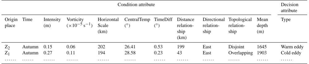
Z2 Autumn 0.15 0.06 202 26.41 0.53 199 East Disjoint 1645 Warm eddy
Z1 Autumn 0.27 0.11 194 28.58 0.23 43 East Overlapping 1903 Cold eddy
. . . .
12. Topological relationship (Topology) to the reference eddy, which can be represented by the RCC-8 Model (Randell et al., 1992; Randell and Cohn, 1989) as dis-joint or overlapping.
3 Results
3.1 Attribute selection
According to the methodology introduced in Sect. 2, the spatial-temporal relationship among mesoscale eddies in the SCS are described quantitatively by the twelve attributes specified in Sect. 2.2.3. They are discretised, if continuous, and then being imported into a decision table as condition attributes. A decision attribute is selected depending on the specific concern in each table, resulting in the minimal tribute reducts that are distinct according to the decision at-tribute. As a result, for each issue, rules extracted by rough set theory may be different. The place of origin of an eddy
is selected as decision attribute in Table 2, in order to extract the corresponding rules from spatial-temporal relationships among eddies generated in all 4 zones of the SCS (Fig. 1). The generating season is selected as decision attribute in Ta-ble 3, for investigating seasonal variation of the rules. And the type of eddy (warm/cold eddy) is selected as decision at-tribute in Table 4, where the rules between the two types of eddies are focused on.
Table 5. Spatial-temporal rules extracted from typical
mesoscale-eddy states in 4 zones of the SCS.
No. Spatial-temporal rule Certainty Coverage level % level %
1 Type(Cold Eddy) AND Vorticity([0.7×10⁻⁶,*)) AND HorizontalScale ([*,173)) AND CentralTemp([*,26.92)) =>Zone(Z1)
100 15.5
2 Time(Winter) AND Type(Cold Eddy) AND Vorticity([0.7×10⁻⁶,*)) AND CentralTemp([*,26.92)) =>Zone(Z1)
100 14.3
3 Type(Warm Eddy) AND Intensity([*,0.08)) AND Vorticity([*,0.7×10−6))AND CentralTemp([26.92,28.53)) =>Zone(Z3)
100 13.3
4 Time(Winter) AND Vortic-ity([*, 0.7×10⁻⁶))AND CentralTemp([26.92,28.53)) =>Zone(Z3)
100 13.3
5 Time(Summer) AND HorizontalScale([195,*)) AND Depth([900, 2400]) =>Zone(Z4)
100 11.9
Note: ”[ ]” represents the closed interval, “( )” the open interval, “*” the infinite inter-val, as follows.
3.2 Extraction of spatial-temporal rules of mesoscale eddies in the SCS
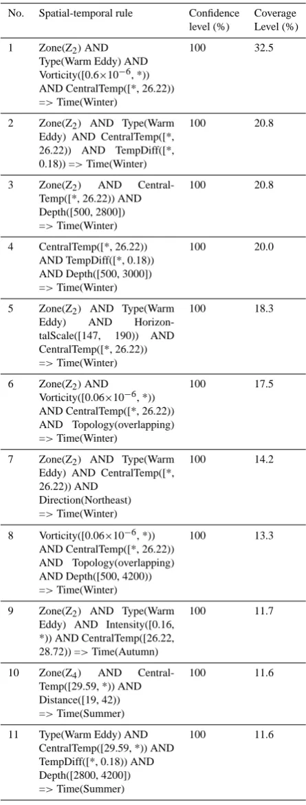
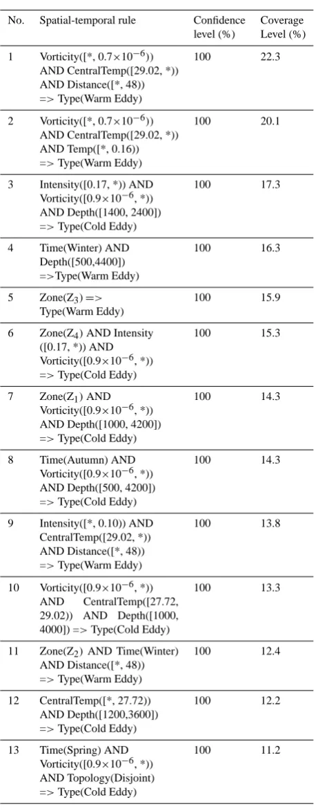
Tables 5–7 show the corresponding spatial-temporal rules extracted from three decision tables (Tables 2–4), in which the decision-making attributes are place of origin, generating season and eddy type, respectively. All the rules have a cov-erage level of more than 10 % and a certainty level of 100 %, respectively, being arrayed in descending order by coverage level. In all, 5 kinds of rules are extracted in Table 5, 11 in Table 6, and 13 in Table 7, respectively.
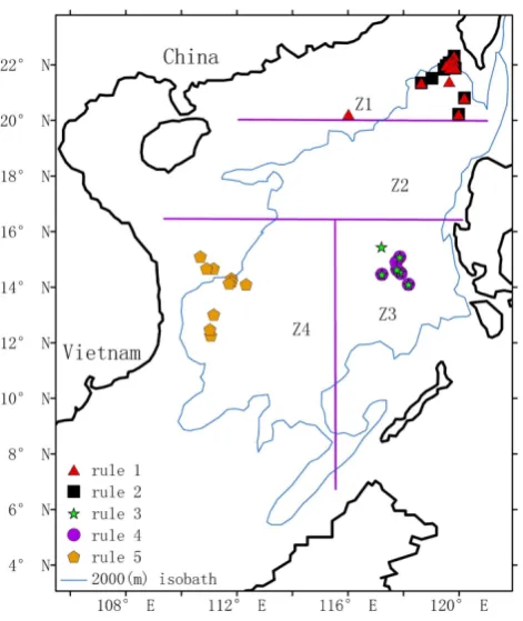
The typical eddy-states following all rules in Table 5 are detected and presented in Fig. 6. There are two of five rules in zone Z1of the SCS, two in zone Z3, 1 in zone Z4and none in zone Z2, respectively. Cold-eddy states following Rule 1 are distributed southwest of Taiwan Island around 2000 m isobaths (zone Z1). It is obvious that most of the states follow both Rules 1 and 2 in this zone, except for one state following Rule 1 merely and one following Rule 2 merely. In Z3zone, all the states are in 4000 m-and-deeper region of the basin, and follow both Rules 3 and 4 except one state following
Table 6. Spatial-temporal rules extracted from typical
mesoscale-eddy states s in 4 seasons.
No. Spatial-temporal rule Confidence Coverage level (%) Level (%)
1 Zone(Z2)AND Type(Warm Eddy) AND Vorticity([0.6×10⁻⁶, *)) AND CentralTemp([*, 26.22)) =>Time(Winter)
100 32.5
2 Zone(Z2) AND Type(Warm Eddy) AND CentralTemp([*, 26.22)) AND TempDiff([*, 0.18)) =>Time(Winter)
100 20.8
3 Zone(Z2) AND Central-Temp([*, 26.22)) AND Depth([500, 2800]) =>Time(Winter)
100 20.8
4 CentralTemp([*, 26.22)) AND TempDiff([*, 0.18)) AND Depth([500, 3000]) =>Time(Winter)
100 20.0
5 Zone(Z2) AND Type(Warm Eddy) AND Horizon-talScale([147, 190)) AND CentralTemp([*, 26.22)) =>Time(Winter)
100 18.3
6 Zone(Z2)AND
Vorticity([0.06×10⁻⁶, *)) AND CentralTemp([*, 26.22)) AND Topology(overlapping) =>Time(Winter)
100 17.5
7 Zone(Z2) AND Type(Warm Eddy) AND CentralTemp([*, 26.22)) AND
Direction(Northeast) =>Time(Winter)
100 14.2
8 Vorticity([0.06×10⁻⁶, *)) AND CentralTemp([*, 26.22)) AND Topology(overlapping) AND Depth([500, 4200)) =>Time(Winter)
100 13.3
9 Zone(Z2) AND Type(Warm Eddy) AND Intensity([0.16, *)) AND CentralTemp([26.22, 28.72)) =>Time(Autumn)
100 11.7
10 Zone(Z4) AND Central-Temp([29.59, *)) AND Distance([19, 42)) =>Time(Summer)
100 11.6
11 Type(Warm Eddy) AND CentralTemp([29.59, *)) AND TempDiff([*, 0.18)) AND Depth([2800, 4200]) =>Time(Summer)
Table 7. Spatial-temporal rules extracted from typical states of two
types of mesoscale eddy.
No. Spatial-temporal rule Confidence Coverage level (%) Level (%)
1 Vorticity([*, 0.7×10⁻⁶))
AND CentralTemp([29.02, *)) AND Distance([*, 48)) =>Type(Warm Eddy)
100 22.3
2 Vorticity([*, 0.7×10⁻⁶))
AND CentralTemp([29.02, *)) AND Temp([*, 0.16)) =>Type(Warm Eddy)
100 20.1
3 Intensity([0.17, *)) AND Vorticity([0.9×10⁻⁶, *)) AND Depth([1400, 2400]) =>Type(Cold Eddy)
100 17.3
4 Time(Winter) AND Depth([500,4400]) =>Type(Warm Eddy)
100 16.3
5 Zone(Z3)=> Type(Warm Eddy)
100 15.9
6 Zone(Z4)AND Intensity ([0.17, *)) AND Vorticity([0.9×10⁻⁶, *)) =>Type(Cold Eddy)
100 15.3
7 Zone(Z1)AND Vorticity([0.9×10⁻⁶, *)) AND Depth([1000, 4200]) =>Type(Cold Eddy)
100 14.3
8 Time(Autumn) AND Vorticity([0.9×10⁻⁶, *)) AND Depth([500, 4200]) =>Type(Cold Eddy)
100 14.3
9 Intensity([*, 0.10)) AND CentralTemp([29.02, *)) AND Distance([*, 48)) =>Type(Warm Eddy)
100 13.8
10 Vorticity([0.9×10⁻⁶, *)) AND CentralTemp([27.72, 29.02)) AND Depth([1000, 4000]) =>Type(Cold Eddy)
100 13.3
11 Zone(Z2)AND Time(Winter) AND Distance([*, 48)) =>Type(Warm Eddy)
100 12.4
12 CentralTemp([*, 27.72)) AND Depth([1200,3600]) =>Type(Cold Eddy)
100 12.2
13 Time(Spring) AND Vorticity([0.9×10⁻⁶, *)) AND Topology(Disjoint) =>Type(Cold Eddy)
100 11.2
Rule 3 only and one following Rule 4 only. There is a warm eddy southwest of Luzon Island besides the famous Luzon Cold Eddy, located northwest of Luzon Island.
Spatial-temporal rules extracted from typical mesoscale-eddy states occurring in the four seasons are presented in Ta-ble 6. A total of 8 rules are extracted in winter, 2 in summer, 1 in fall and none in spring, respectively. Spatial distribution of the states following all 11 rules is shown in Fig. 7a in win-ter, 7b in summer and 7c in fall. No eddy state is extracted in spring. As Fig. 7a shows, all the states, in winter, are con-centrated around the western 2000 m isobaths of the northern basin (both zones Z1and Z2)with an exception of one state in the basin center (zone Z3). There are many more states of eddies in winter than the other seasons.
In Fig. 7a, two states obey Rules 1 and 2 together in zone Z2. Another two obey Rules 2 and 3 together in zone Z2. These four states are located in the eastern Paracel Is-land, maybe originating from the Xisha Warm Eddy AE1 in D. Wang et al. (2008). Two states obey Rules 6 and 7 to-gether: one in zone Z1, another in zone Z2. Furthermore, several eddy states obey three rules together, including two obeying Rules 1, 6 and 7 together in zone Z2, which maybe originates from Warm Eddy AE1 detected by D. Wang et al. (2008), and three obeying Rules 2, 6 and 7 together on the boundary of zone Z2towards zone Z1, which maybe origi-nate from another Warm Eddy AE2 detected by D. Wang et al. (2008). Three states obey Rules 4 and 8 together in zone Z1. In addition, four obey Rules 2, 3 and 8 together in zone Z2, and two states obey four rules (Rules 1, 3, 6 and 7) to-gether in zone Z2.
In summer, the typical states of eddies become less ob-vious, as shown in Table 6. Most of the states, in Fig. 7b, are distributed around the western 2000 m isobaths with one exception in the central basin (zone Z3). There are two clus-ters of eddy states off the Vietnam coast, eight states over the shelf of northern Vietnam (<2000 m), and seven in the 2000 m and deeper region off southern Vietnam in zone Z4. Only two obey both summer rules together, one is in shallow water off northern Vietnam coast, the other is in deep wa-ter off southern Vietnam Peninsula. Besides, there are three warm-eddy states located in north of the basin, the bound-ary of zones Z1and Z2. NLOM displaces the wind jet flow northwards to 13–14◦N (compared with the observed loca-tion 10.5–11◦N) so that the two clusters are distributed either side of 14◦N.
In fall, all ten eddy states are around the western boundary of 2000 m isobaths of the northern basin (zone Z2) exclu-sively, as shown in Fig. 7c, one half are in north of the zone, the other half in the south. This season has the least eddy states annually. These states form four clusters. Two of them are off west Luzon Strait, another two are composed by 4 states off the southeast of Hainan Island.
(a) (b) (c)
(d) (e)
Fig. 5. Comparison of 5-days NLOM SSHA contours with AVISO SLA image in the SCS. Four deterministic eddies are marked as Warm
Eddy off the Luzon Strait (red capital A), the West Luzon Eddy (red capital B), the Warm Eddy near Xisha Island (red capital C) and the Eddy Pair Offshore from Vietnam (red capital D).
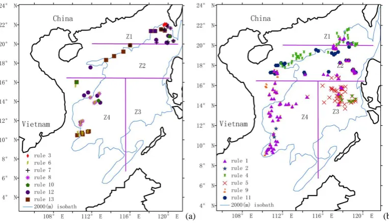
warm-eddy states, and 7 rules (Rules 3, 6, 7, 8, 10, 12 and 13) for cold-eddy states. Spatial distribution of cold-eddy states is shown in Fig. 8a and warm-eddy states in Fig. 8b.
All cold-eddy states are distributed as a band along the western 2000 m isobaths (Fig. 8a) from west of Luzon Strait to the southeast of Hainan Island, and to offshore of Viet-nam; they are also revealed recently by both model and satel-lite data (Xiu et al., 2010). In zone Z1, two cold-eddy states obey Rules 7 and 13 together in spring, five obey Rules 7 and 8 together in fall and two obey Rules 12 and 13 together in spring, other than one cold-eddy state obeys Rules 7, 8 and 10 together in fall. Figure 8a also shows that the states fol-lowing Rule 3 seldom exist southwest of Taiwan Island. In zone Z2, one cold-eddy state obeys Rules 7 and 13 together. Three obey Rule 13 in spring, and one obeys Rule 12. None is in zone Z3. In zone Z4, two clusters of states are sepa-rated by the wind jet along 13–14◦N. Four cold-eddy states following Rule 12 are located at the northern wind jet. Six cold-eddy states follow Rules 6 and 8 together in fall, being distributed on each side of the jet as parts of the two clus-ters, respectively. And one state follows Rules 6, 8 and 10 together in fall on the southern side of the jet flow.
Fig. 6. Spatial distribution of typical mesoscale-eddy states in the
SCS extracted from Table 5. (Blue line is 2000 m isobaths.)
4 Discussion
Orographic wind is induced by the Cordillera on the south-west of Taiwan Island in winter. It makes cold water in the subsurface upwelling and forms a cold-eddy core due to the Ekman pumping effect (Qu, 2000). Thus, cold-eddy states on the northeastern tip of 2000 m isobaths in Fig. 6 may be induced by this orographic wind stress curl. G. Wang et al. (2008) reveal that the winter gap winds in the mountain-ous island chain along the eastern boundary of the SCS are intrinsic regional features of the monsoon due to orographic effects, spinning up cold and warm eddies west of Luzon Is-land. In summer, the eddy pair offshore from Vietnam in-duced by a wind jet, as is well known, has the same attributes in horizontal scale and the water depth of eddy core (Rule 5 in Table 5).
In winter, the Kuroshio intrusion plays a major role on mesoscale eddies in the northern SCS (e.g. Su, 2004; Wu and Chiang, 2007; Zhuang et al., 2010). Frontal instability at the Kuroshio intrusion could be one mechanism in eddy shedding (Wang et al., 2000; Su, 2004). In Fig. 7a, a certain warm-eddy states have the possibility to be shed from the Kuroshio meander near west of Luzon Strait. Several pre-vious studies conclude that, off central Vietnam, there is a cyclonic gyre north of about 12◦N, but an anti-cyclonic gyre to the south (Kuo et al., 2000; Xie et al., 2003). Accompa-nying these gyres is a northward orographic wind jet turning
offshore from the Vietnam coast near 12◦N. In Fig. 7b, the typical warm-eddy states are distributed not only south of the jet flow induced by intraseasonal wind stress, but also in the northern shallow water; it is unclear how eddy is generated; this should be a focus of future study. In Fig. 7c, the south partition seems to derive from two warm eddies AE1 and AE2 near Paracel Island in D. Wang et al. (2008).
All of cold-eddy states appear in spring and fall, neither summer nor winter, and they converge on the northern tip of the basin and west of Luzon Strait, as shown in Fig. 8a; they are induced by wind stress curl resulting from the blockage effect of Cordillera on the southwest of Taiwan Island (Qu, 2000; Su, 2004) or the net water transport into the SCS via the Luzon strait (Su, 2004). Lack of a cold-eddy rule in win-ter, may result from the rules’ coverage level being less than 10 %, not indicative of no cold eddy at all. In zone Z4, the cold-eddy states located at both northern and southern sides of the Vietnam jet flow only occur in fall. Wind forcing plays a major role in their generation (Zhuang et al, 2010). Four cold-eddy states obey Rules 6 and 13 together in spring, lo-cated only on the southern wind jet off the Vietnam coast. It is unclear why a cold eddy occurs in this season, and no pre-vious study focuses on this question. Oceanographers should pay more attention to this phenomenon in future study. In Fig. 8b, the two-strip distribution is in good agreement with the spatial pattern achieved by both model and satellite ob-servations (Xiu et al., 2010) and total eddy energy achieved by the intraseasonal variability of SSH (Zhuang et al., 2010). In winter the Kuroshio intrusion induces warm eddies west of Luzon Strait and their evolution, and the Dongsha warm cur-rent induces frontal warm eddies (Su, 2004) near Pratas Is-land. Wind forcing converges on the upper-layer warm water and downwells under the Ekman pumping effect (Qu, 2000). Downwelling brings warm water from surface to the deep creating warm core eddies such as the West Luzon Eddy. Eddy states following Rules 4 and 5 in Table 7 off south-western Luzon Island are considered as being induced by the interaction between strong barotropic shelf currents and the local topography (Xiu et al., 2010). There is no warm-eddy state in the northern tip of 2000 m isobaths (southwest of Tai-wan Island or west of Luzon Strait), as is clear in Fig. 8a, maybe due to lack of negative wind stress curl.
There is a phenomenon that some typical mesoscale-eddy states follow two rules or more in Figs. 6–8, respectively, indicating they have much stronger regularity in spatial-temporal distribution. From the above analysis, we find that the typical cold-eddy states located southwest of Taiwan Is-land, namely the northeastern tip of the basin, appear in winter (Fig. 6). The typical warm-eddy states are distributed either southwest of Luzon Island, the deepest region of the basin, or the western edge of 2000 m isobaths. It is shown in Table 7 that no rule can be co-followed by the two types of eddies.
(a) (b) (c)
Fig. 7. Spatial distributions of typical states of two types of mesoscale eddy in (a) winter, (b) summer and (c) fall in the SCS extracted from
Table 6. No state is extracted in spring. (Blue line is 2000 m isobaths.)
(a) (b)
Fig. 8. Spatial distribution of all typical (a) cold-eddy states and (b) warm-eddy states in the SCS extracted from Table 7. (Blue line is
2000 m isobaths.)
simulation and satellite observation. Some of their conclu-sions can be replicated in our study, as the following exam-ples:
1. Through analyzing 5-yr T/P data, Wang et al. (2000) point out that mesoscale eddies in the SCS are active along the western 2000 m isobaths and the NE-SW ori-ented band from south of Luzon Strait to 11◦N around the eastern Vietnam Peninsula. This is also revealed by Lin et al. (2007) through statistical analysis of 10-yr T/P data and Wang (2004) through statistical analysis of 8-yr T/P data. In our study this spatial feature of eddies is confirmed one more time, as shown in Fig. 8b. In
this Figure, warm-eddy states are located in the NW-SE oriented band, which confirms the conclusion in Lin et al. (2007) that there are warm eddies in the region (14–15◦N, 118–120◦E) exclusively, but no cold eddy occurs.
2. Cheng et al. (2005) conclude that warm eddies are dis-tributed north of 18◦N, which is followed by Rule 1, 2, 5 and 7 in Table 5 and Rule 11 in Table 6. In Fig. 8b, these states are in the western zone Z2(18–20◦N). 3. Most mesoscale eddies appear off the eastern
northeastern SCS, while they are inactive in the south-eastern SCS (e.g. Wang, 2004; Lin et al., 2007; Cheng et al., 2005). This is confirmed in Fig. 6.
4. D. Wang et al. (2008) examine warm eddies AE1 and AE2 in the northeastern SCS during the winter of 2003– 2004. We can confirm that the six states of eddy AE1 in Figs. 2 and 4 of D. Wang et al. (2008) follow Rules 1 and 3 together in Table 5 and Rules 4 and 11 together in Table 6, while none of rules is followed by states of eddy AE2. AE2 locates in zone Z1, as shown in Fig. 6. No rule can be extracted among warm-eddy states in this zone in winter other than Rule 1 of Table 6. It should be pointed out that we are not able to obtain the Euclidean distance, directional relationship and topological rela-tionship of the two eddies. Thus only some of rules in Tables 4–6 could be confirmed by D. Wang et al. (2008). However, there are several features achieved in our study that were not paid enough attention in previous works. In winter, warm eddies, as is well known, are generated in the northeastern SCS resulting from the frequent Kuroshio in-trusion, thus most oceanographers focus on their generating mechanism, evolving process, and so on. Whereas, a few rules extracted in this zone are followed by cold eddies in winter, indicating cold eddies may be well-regulated in the region. Meanwhile, west of Luzon Island, the famous Luzon cold eddy is focused. Several rules, however, are achieved for warm eddies in this zone, indicating warm eddies may be well-regulated in the region as well. Otherwise, warm eddies are distributed not only on the jet flow off southern Vietnam induced by intraseasonal wind stress in summer-fall, but also on the northern shallow water, which should be a focus of future study. Similarly, cold eddies are also located at both northern and southern sides of the Vietnam jet flow in fall. And there are cold eddies generated off southern Vietnam in spring. These are interesting but no studies have been carried out; we suggest that these eddies should be studied.
Otherwise, the approach requires to select the correspond-ing spatial-temporal relationships among mesoscale eddies according to each issue. It is also worth noting that the raw data used in this study is derived from numerical modeling. Some eddies with a shorter life-time or smaller horizontal scale may not be included, as a result of not being identified. So the number of eddies analyzed is fewer than the actual to-tal. In the future, the rough set approach will be improved by supplementing data acquired in different sea areas and sea-sons into the database, selecting appropriate attribute factors that can better reflect spatial-temporal relationships among eddies, and applying other discretization and reducts algo-rithms based on rough set theory. Comparison of the results derived from different scenarios would help yield more prac-tically significant rules.
5 Conclusions
In this paper, a rough set theory is introduced to represent spatial-temporal relationships and extract the corresponding rules from typical mesoscale-eddy states in the SCS. These rules clearly confirm spatial-temporal distribution patterns and features of these states. Three decision attributes are adopted in this study, which make the approach flexible in retrieving spatial-temporal rules with different features. The results demonstrate that this approach is effective, and there-fore provides a powerful approach to there-forecasts in future stud-ies. Spatial-temporal rules in the SCS indicate that warm ed-dies following the rules are generally in the southeastern and central SCS around 2000 m isobaths in winter. Their inten-sity and vorticity are weaker than those of cold eddies. They usually move a shorter distance. By contrast, cold eddies are in 2000 m and deeper regions of the southwestern and north-eastern SCS in spring and fall. Their intensity and vorticity are strong. Usually they move a long distance. In winter, a few rules are followed by cold eddies in the northern tip of the basin and southwest of Taiwan Island rather than warm eddies, indicating cold eddies may be well-regulated in the region. Several warm-eddy rules are achieved west of Lu-zon Island, indicating warm eddies may be well-regulated in the region as well. Otherwise, warm and cold eddies are distributed not only in the jet flow off southern Vietnam in-duced by intraseasonal wind stress in summer-fall, but also in the northern shallow water, which should be a focus of future study.
Acknowledgements. This work was fully supported by the
National Science Fund (project Number: 41071250), and the National 863 High Technology Programs of China (Project No. 2011BAH23B04), and was granted from an independent innovation project of State Key Laboratory of Resource and Envi-ronment Information System, CAS (Project No. 088RA500KA). The authors appreciate comments from reviewers and readers.
Edited by: J. M. Huthnance
References
Bai, H., Ge, Y., Wang, J., and Liao, Y.: Using rough set theory to identify villages affected by birth defects: the example of Hes-hun, Shanxi, China, Int. J. Geogr. Inf. Sci., 24, 559–576, 2010. Cheng, X., Qi, Y., and Wang, W.: Seasonal and Interannual
Vari-abilities of Mesoscale Eddies in South China Sea, J. Trop. Oceanogr., 24, 51–59, 2005.
Fang, G., Chen, H., Wei, Z., Wang, Y., Wang, X., and Li, C.: Trends and interannual variability of the South China Sea surface winds, surface height, and surface temperature in the recent decade, J. Geophys. Res. 111, C11S16, doi:10.1029/2005JC003276, 2006. Fayyad, U. M. and Irani, K. B.: On the handling of continuous-valued attributes in decision tree generation, Mach. Learn., 8, 87–102, 1992.
Proceedings of the 13th International Joint Conference on Artifi-cial Intelligence, IJCAI-93, 1993.
He, Z., Wang, D., and Hu, J.: Features of eddy kinetic energy and variations of upper circulation in the South China Sea, Acta Oceanol. Sinica, 21, 305–314, 2002 (in Chinese with English ab-stract).
Hetland, R. H., Hsueh, Y., Leben, R. R., and Niiler, P. P.: A loop current-induced jet along the edge of the West Florida shelf, Geo-phys. Res. Lett., 26, 2239–2242, 1999.
Hu, J., Kawamura, H., Hong, H., Kobashi, F., and Wang, D.: 3–6 months variation of sea surface height in the South China Sea and its adjacent ocean, J. Oceanogr., 57, 69–78, 2001.
Hurlburt, H. E. and Thompson, J. D.: A numerical study of loop current intrusions and eddy shedding, J. Phys. Oceanogr., 10, 1611–1651, 1980.
Hwang, C., Wu, C. R., and Kao, R.: TOPEX/Poseidon observations of mesoscale eddies over the Subtropical Counter Current: kine-matic characteristics of an anticyclonic eddy and a cyclonic eddy, J. Geophys. Res., 109, C08013, doi:10.1029/2003JC002026, 2004.
Jia, Y. and Liu, Q.: Eddy shedding from the Kuroshio bend at Luzon Strait, J. Oceanogr., 60, 1063–1069, 2004.
Jia, Y., Liu, Q., and Liu, W.: Primary studies of the mechanism of eddy shedding from the Kuroshio bend in Luzon Strait, J. Oceanogr., 61, 1017–1027, 2005.
Komorowski, J., Pawlak, Z., Polkowski, L., and Skowron, A.: Rough sets: A tutorial, in: Rough fuzzy hybridization: a new trend in decision-making, edited by: Pal, S. and Skowron, A., Singapore, Springer-Verlag, 3–93, 1999.
Kuo, N. J., Zheng, Q., and Ho, C. R.: Satellite observation of up-welling along the western coast of the South China Sea, Remote Sens. Environ., 74, 463–470, 2000.
Leung, Y. and Li, D.: Maximal consistent block technique for rule acquisition in incomplete information systems, Inf. Sci., 153, 85– 106, 2003.
Li, L.: A review on mesoscale oceanographical phenomena in the South China Sea, J. Oceanogr. Taiwan, 21, 265–274, 2002 (in Chinese with English abstract).
Li, L. and Wu, B.: A Kuroshio loop in South China Sea?, J. Oceanogr. Taiwan, 8, 89–95, 1989 (in Chinese with English ab-stract).
Li, L., Nowlin Jr., W. D. and Su, J.: Anticyclonic rings from the Kuroshio in the South China Sea, Deep-Sea Res. Pt. I 45, 1469– 1482, 1998.
Lin, P., Wang, F., Chen, Y., and Tang, X.: Temporal and spatial variation characteristics on eddies in the South China Sea I. Sta-tistical analyses, Acta Oceanol. Sinica, 29, 14–22, 2007. Liu, Q., Jiang, X., Xie, S., and Liu, W.: A gap in the Indo-Pacific
warm pool over the South China Sea in boreal winter: Seasonal development and interannual variability, J. Geophys. Res., 109, C07012, doi:10.1029/2003JC002179, 2004.
Metzger, E. J. and Hurlburt, H. E.: The nondeterministic nature of Kuroshio penetration and eddy shedding in the South China Sea, J. Phys. Oceanogr., 31, 1712–1732, 2001.
Miao, D. and Li, D.: Rough Sets Theory Algorithms and Applica-tions, TsingHua University Press, Beijing, 2008.
Nguyen, H. S. and Skowron, A.: Quantization of real-valued at-tributes, in: Proceeding 2nd International Joint Conference on Information Sciences, Wrightsville Beach, NC, 34–37, 1995.
Pawlak, Z.: Rough sets, Int. J. Parallel. Prog., 11, 341–356, 1982. Pawlak, Z.: Rough Sets: Theoretical Aspects of Reasoning about
Data, Kluwer Academic Publishers, Boston, 1991.
Pawlak, Z.: Bayes’ theorem revised- the rough set view, in: Pro-ceedings of International Workshop on Rough Set Theory and Granular Computing (RSTGC 2001), Matshue, Shimane, Japan, 1–8, 2001.
Polkowski, L. and Skowron, A.: Rough Sets in Knowledge Discov-ery 1: Methodology and Applications, 2: Applications, Physica-Verlag, Heidelberg, 1998.
Polkowski, L., Tsumoto, S., and Lin, T.: Rough Set Methods and Applications, Physica-Verlag, Heidelberg, 49–88, 2000. Qhrn, A.: Discernibility and rough sets in medicine: tools and
appli-cation, Norwegian University of Science and Technology, Nor-way, 41–51, 1999.
Qu, T.: Upper-layer circulation in the South China Sea, J. Phys. Oceanogr., 30, 1450–1460, 2000.
Randell, D. A. and Cohn, A. G.: Modelling topological and met-rical properties in physical processes, in: Proceedings of the 1st International Conference on the Principles of Knowledge Rep-resentation and Reasoning, Morgan Kaufmann Publishers, San Francisco, 55–66, 1989.
Randell, D. A., Cui, Z., and Cohn, A. G.: A spatial logic based on regions and connection, in: Proceedings of the 3rd International Conference on Principles of Knowledge Representation and Rea-soning, Morgan Kaufmann Publishers, San Francisco, 165–176, 1992.
Roemmich, D. and Gilson, J.: Eddy transport of heat and thermo-cline waters in the North Pacific: a key to interannual/decadal climate variability, J. Phys. Oceanogr., 31, 675–687, 2001. Skowron, A.: Synthesis of adaptive decision systems from
experi-mental data, in: Proceedings of the Fifth Scandinavian Confer-ence on Artificial IntelligConfer-ence, number 28 in Frontiers in Arti-ficial Intelligence and Applications, edited by: Aamodt, A. and Komorowski, J., IOS Press, 220–238, 1995.
Skowron, A.: Rough sets and Boolean reasoning, in: Granular Computing: An Emerging Paradigm, edited by: Pedrycz, W., Physica-Verlag, Heidelberg, 95–124, 2001.
Su, J.: Overview of the South China Sea circulation and its influence on the coastal physical oceanography outside the Pearl River Es-tuary, Cont. Shelf Res., 24, 1745–1760, 2004.
Su, J., Lu, J., Hou, Y., Fang, G., Wei, Z., and Yin, B.: Analysis of satellite-tracked drifting buoys in the South China Sea, Oceanol. Limnol. Sinica, 33, 121–127, 2002 (in Chinese with English ab-stract).
Wang, D., Xu, H., Lin, J., and Hu, J.: Anticyclonic eddies in the northeastern South China Sea during winter 2003/2004, J. Oceanogr., 64, 925–935, 2008.
Wang, G.: Discussion on the Movement of Mesoscale Eddies in the South China Sea, Ph.D. Dissertation, Ocean University of China, Qingdao, 2004.
Wang, G., Su, J., and Chu, P.: Mesoscale eddies in the South China Sea observed with altimeter data, Geophys. Res. Lett., 30, 2121, doi:10.1029/2003GL018532, 2003.
Wang, G., Chen, D., and Su, J.: Generation and life cycle of the dipole in the South China Sea summer circulation, J. Geophys. Res., 111, C06002, doi:10.1029/2005JC003314, 2006.
38, 726–732, doi:10.1175/2007JPO3868.1, 2008.
Wang, G. Y.: Rough Set Theory and Knowledge Acquisition, Xi’an: Xi’an Jiaotong University Press, 2001 (in Chinese).
Wang, L., Koblinsky, C. J., and Howden, S.: Mesoscale variability in the South China Sea from the TOPEX/Poseidon altimetry data, Deep-Sea Res Pt. I, 47, 681–708, 2000.
White, W. B.: Tropic coupled Rossby waves in the Pacific ocean-atmosphere system, J. Phys. Oceanogr., 30, 1245–1264, 2000. Wu, C. and Chang, C. W. J.: Interannual variability of the South
China Sea in a data assimilation model, Geophys. Res. Lett., 32, L17611, doi:10.1029/2005GL023798, 2005.
Wu, C. and Chiang, T.: Mesoscale eddies in the northern South China Sea, Deep-Sea Res. Pt. II, 54, 1575–1588, 2007.
Wu, C., Tang, T., and Lin, S.: Intra-seasonal variation in the velocity field of the northeastern South China Sea, Cont. Shelf Res., 25, 2075–2083, 2005.
Wyrtki, K.: Physical oceanography of the southeast Asian waters, NAGA report, Vol. 2, Scientific results of marine investigation of the South China sea and the Gulf of Thailand, Scripps Institution of Oceanography, La Jolla, Calif., 195 pp., 1961.
Xie, S., Xie, Q., Wang, D., and Liu, W.: Summer upwelling in the South China Sea and its role in regional climate variations, J. Geophys. Res., 108, 3261, doi:10.1029/2003JC001867, 2003. Xiu, P., Chai, F., Shi, L., Xue, H., and Chao, Y.: A census of eddy
activities in the South China Sea during 1993–2007, J. Geophys. Res., 115, C03012, doi:10.1029/2009JC005657, 2010.
Xu, X., Qiu, Z., and Chen, H.: The general descriptions of the hor-izontal circulation in the South China Sea, in: Proceedings of the 1980 Symposium on Hydrometeorology, Chinese Society of Oceanology and Limnology, Science Press, Beijing, 137–145, 1982.
Yang, K., Shi, P., Wang, D., and Qi, Y.: Numerical study about the mesoscale multi-eddy system in the northern South China Sea in winter, Acta Oceanol. Sinica, 22, 27–34, 2000 (in Chinese with English abstract).
Yasdi, R.: Combining rough sets learning and neural learning: method to deal with uncertain and imprecise information, Neu-ralcomputing, 7, 61–84, 1996.
Yuan, D., Han, W., and Hu, D.: Surface Kuroshio path in the Luzon Strait area derived from satellite remote sensing data, J. Geophys. Res., 111, C11007, doi:10.1029/2005JC003412, 2006.
Yuan, D., Han, W., and Hu, D.: Anti-cyclonic eddies northwest of Luzon in summer-fall observed by satellite altimeters, Geophys. Res. Lett., 34, L13610, doi:10.1029/2007GL029401, 2007. Yuan, S. Y. and Wang, Z. Z.: Topography forced Rossby waves in
the section from Xisha to Dongsha Islands, Trop. Oceanol., 5, 1–6, 1986 (in Chinese with English abstract).