www.the-cryosphere.net/11/841/2017/ doi:10.5194/tc-11-841-2017
© Author(s) 2017. CC Attribution 3.0 License.
Internal structure of two alpine rock glaciers investigated by
quasi-3-D electrical resistivity imaging
Adrian Emmert and Christof Kneisel
Institute of Geography and Geology, University of Würzburg, 97074, Germany Correspondence to:Adrian Emmert ([email protected]) Received: 31 May 2016 – Discussion started: 4 July 2016
Revised: 30 November 2016 – Accepted: 2 December 2016 – Published: 30 March 2017
Abstract.Interactions between different formative processes are reflected in the internal structure of rock glaciers. There-fore, the detection of subsurface conditions can help to en-hance our understanding of landform development. For an assessment of subsurface conditions, we present an analy-sis of the spatial variability of active layer thickness, ground ice content and frost table topography for two different rock glaciers in the Eastern Swiss Alps by means of quasi-3-D electrical resistivity imaging (ERI). This approach enables an extensive mapping of subsurface structures and a spatial overlay between site-specific surface and subsurface charac-teristics. At Nair rock glacier, we discovered a gradual de-scent of the frost table in a downslope direction and a con-stant decrease of ice content which follows the observed sur-face topography. This is attributed to ice formation by re-freezing meltwater from an embedded snow bank or from a subsurface ice patch which reshapes the permafrost layer. The heterogeneous ground ice distribution at Uertsch rock glacier indicates that multiple processes on different time do-mains were involved in the development. Resistivity values which represent frozen conditions vary within a wide range and indicate a successive formation which includes several advances, past glacial overrides and creep processes on the rock glacier surface. In combination with the observed to-pography, quasi-3-D ERI enables us to delimit areas of ex-tensive and compressive flow in close proximity. Excellent data quality was provided by a good coupling of electrodes to the ground in the pebbly material of the investigated rock glaciers. Results show the value of the quasi-3-D ERI ap-proach but advise the application of complementary geo-physical methods for interpreting the results.
1 Introduction
Geophysical techniques such as electrical resistivity to-mography (ERT), seismic refraction toto-mography (SRT) or ground-penetrating radar (GPR) are widely used today and provide a multi-dimensional investigation of subsurface con-ditions in permafrost environments and corresponding land-forms. For rock glaciers and similar periglacial landforms, geophysical investigations enable an assessment of the sub-surface material composition and to distinguish between frozen and unfrozen areas (e.g. Schneider et al., 2013; Musil et al., 2006). This information can be used to investigate inferences with creep velocities (Hausmann et al., 2012; Kneisel and Kääb, 2007) or to reveal glacier–permafrost in-teractions during the development of rock glaciers (see Dusik et al., 2015; Krainer et al., 2012; Ribolini et al., 2010).
In contrast to those numerous one- or two-dimensional field studies, in which vertical and lateral variations of re-sistivity distribution could be detected, three-dimensional in-vestigations are sparse in the field of periglacial geomor-phology. Approaches were presented by Scapozza and Lai-gre (2014) and Langston et al. (2011), who graphically com-bined results from 2-D ERT surveys to three-dimensional fence diagrams. However, these approaches do not take into account the actual three-dimensionality of the subsurface re-sistivity distribution and the so-called “3-D effects”, which result from small-scale heterogeneities (Loke et al., 2013). This is achieved by running a 3-D inversion on a data set consisting of multiple intersecting 2-D data sets (“quasi-3-D” approach), which enables a horizontal mapping of resis-tivity variations, an assessment of the geometry of the de-tected structures and consequently a more realistic character-isation of three-dimensional subsurface conditions (Kneisel et al., 2014; Rödder and Kneisel, 2012).
The objective of this paper is to describe the internal struc-ture of two morphologically different rock glaciers with re-gard to frost table variations, active layer thickness (ALT), ice content and ground ice genesis. We therefore analyse the three-dimensional subsurface resistivity distribution which is modelled by quasi-3-D electrical resistivity imaging (ERI) and the results from additionally performed comparative sur-veys of 2-D ERT and 2-D SRT. Ground truthing is achieved by borehole temperature measurements. We present a qual-itative assessment of ground ice content which we presume is sufficient for interpreting the results regarding rock glacier development. Quantitative assessments, as presented e.g. by Pellet et al. (2016), Hausmann et al. (2012) or Hauck et al. (2011), would additionally require a spatial assessment of porosity.
2 Study sites
The investigated rock glaciers are located in the Eastern Swiss Alps, an area which is well known for the occurrence of permafrost and numerous rock glaciers. The nearby rock glaciers Murtèl and Muragl probably belong to the best
in-vestigated rock glaciers in the European Alps (e.g. Maurer and Hauck, 2007). For the presented study, two landforms described as “pebbly rock glaciers” according to the rela-tively small grain size (dominant clast size <20 cm) of the surface debris (Matsuoka et al., 2005) were chosen. The dis-tance between the two sites is ca. 12 km. In September 2014, one borehole with a depth of 10 m was drilled at Uertsch rock glacier and one borehole with the same depth was drilled at Nair rock glacier. Both boreholes are instrumented with ther-mistor strings with 15 temperature sensors. The temperature sensors are located at the ground surface and 0.2, 0.4, 0.8, 1.2, 1.6, 2, 3, 4, 5, 6, 7, 8, 9 and 10 m below the surface. As a destructive drilling method was applied, no borehole cores are available. Accuracy of the installed sensor type (Dallas, Geoprecision) is±0.25◦C and a temporal resolution of 1 h is provided.
2.1 Nair rock glacier
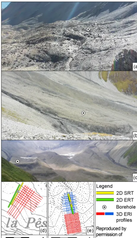
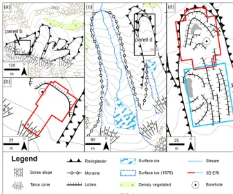
Nair rock glacier (46◦310N, 9◦470E; ca. 2845–2820 m a.s.l.; Fig. 1a) is located at the southern slope of a small high mountain valley near the city of Celerina, Upper Engadine. It is part of a widespread rock glacier assembly at the val-ley slope and roots below a steep talus cone (Figs. 1a, 2a). It is composed of debris material from the sedimentary rocks of the Piz Nair summit area (mainly schist and marlstone). The Alpine Permafrost Index Map (Boeckli et al., 2012) de-scribes the spatial distribution of permafrost in the area of the rock glacier as “permafrost in nearly all conditions”. The investigated rock glacier consists of several adjacent lobes, but our study concentrates on the uppermost eastern lobe, which is about 90 m×80 m in size. The occurrence of perma-nently frozen ground within this part of the rock glacier was reported by Ikeda and Matsuoka (2006), who performed a seismic refraction sounding and one 2-D ERT measurement (specified therein as NN12). Their study describes the rock glacier as “active”, but no flow velocity measurements were published. A glaciation of the site during Little Ice Age (LIA) is not indicated by morphological traces but surface ice is dis-played on ancient topographical maps from ca. 1917 to 1944 at the position of the present talus cones and at the root zone of the rock glacier (Coaz et al., 1925, 1946).
2.2 Uertsch rock glacier
Figure 1.Site overview and measurement set-ups:(a)photo of Nair site;(b, c)photos of Uertsch site;(d)quasi-3-D ERI set-up at Nair;
(e)quasi-3-D ERI set-up at Uertsch_01 (blue lines) and Uertsch_02 (red lines).
glacier (Fig. 2c). Surface ice is displayed on a topographical map from 1878, but pictured there only slightly larger than the extent of the recent ice patch (Coaz and Leuzinger, 1878). A similar lateral moraine is lacking at the eastern edge. Small longitudinal ridges occur in the central part of the rock glacier and several relict lobes in front of the rock glacier indicate a successive formation (Figs. 1c, 2c). On the surface, isolated pioneer plants indicate inactivity. The rock glacier mostly consists of fine-grained schist from the mountain ridge between Piz Üertsch and Piz Blaisun. The rooting zone is part of a wide amphitheatre-like catchment area, where remnant ice from a former glaciation and lateral moraines from the former glacier extent are visible (Figs. 1c, 2c). However, this part is a little cut off from the root zone of
the rock glacier. The Alpine Permafrost Index Map (Boeckli et al., 2012) describes the occurrence of permafrost at the main part of the rock glacier as “permafrost only in very favourable conditions”. Only the area of the rooting zone of the rock glacier is described by the term “permafrost mostly in cold conditions”. The borehole is located in the lower part of the rock glacier, situated at the edge of one of the surface ridges. Some morphometrical attributes (e.g. length, slope aspect, lithology) of the rock glacier were presented by Ikeda and Matsuoka (2006) (specified therein as A8), but no geophysical surveys were published.
3 Methods
The application of geophysical measurements for the de-tection of subsurface conditions is common practice in per-mafrost research (e.g. Hauck, 2013; Kneisel et al., 2008; Otto and Sass, 2006) and therefore only short descriptions of the basic approaches are given here. As the ranges of resistivity values for frozen and unfrozen conditions are partly over-lapping, the application of complementary methods for the detection of frozen subsurface conditions is generally rec-ommended (Schrott and Sass, 2008; Ikeda, 2006).
3.1 Electrical resistivity tomography and quasi-3-D electrical resistivity imaging
Figure 2.Geomorphological setting:(a, b)Nair and(c, d)Uertsch. Legend adapted from Kneisel et al. (1998).
Table 1.Details on quasi-3-D ERI surveys.
NAIR UERTSCH_01 UERTSCH_02
Acquisition dates 12–14 August 2014 11–13 September 2014 26–31 July 2015 Number of grid lines 17 (9X, 8Y) 17 (9X, 8Y) 30 (17X, 13Y) Outline of investigated area 70 m×105 m 70 m×105 m 74 m×105 m
Number of collated 2-D profiles 17 20 60
Array types for 2-D profiles 17 DipDip 17 DipDip+3 WenSl 30 DipDip+30 WenSl Number of data points for inversion 6294 (of max. 6936) 7372 (of max. 7800) 20 523 (of max. 20 880) Absolute error (iteration) 7.77 (5) 5.85 (5) 8.86 (5)
of the quasi-3-D ERI data sets of this study are summarised in Table 1 and the networks of 2-D lines are presented in Fig. 1d, e. Dipole–dipole (DipDip) electrode array was per-formed preferably due to its high resolution in the shallow subsurface and the provided time efficiency by our multi-channel device, but also measurements with the more robust Wenner–Schlumberger (WenSl) array were performed at all sites (and partly included into the 3-D data sets) to reach a higher level of reliability. Where no complete rectangular-shaped grid could be set up due to topographical reasons, the model sections are partly blanked out. The measured appar-ent resistivity data sets were quality checked and bad datum points (standard deviation between reciprocal measurements
>5 %) were deleted manually. The measured 2-D data sets were inverted independently for 2-D interpretation and fur-ther quality checks following the procedures proposed by
values by adjusting the resistivity of the model blocks. These differences are quantified as a mean absolute misfit error value (absolute error). The inversion continues until accept-able convergence between the calculated and the measured data is reached (see Rödder and Kneisel, 2012, for more de-tails on inversion settings). To investigate model reliability, a resolution matrix approach (Hilbich et al., 2009; Wilkin-son et al., 2006; Stummer et al., 2004) was performed on all data sets. This approach provides a measure of the in-formation content of the model cells. It enables an assess-ment of the independence of the modelled resistivity values from neighbouring cells or inversion settings. We also used the approach to evaluate investigation depth. In RES3DINV, the model resolution values are transferred into index values, which additionally take into account the model discretization (Loke, 2015). We followed the suggested index value of 10 as a lower limit to rate model cells as sufficiently resolved. For the conversion from resistivity values to subsurface condi-tions, we applied qualitative attributions based on direct ob-servations by Ikeda and Matsuoka (2006) as their study was performed in the same area, as well as appraisals from our own borehole measurements.
3.2 Seismic refraction tomography
SRT is a suitable complementary method to geoelectrical investigations as it is based on the independent parameter of seismicP-wave velocity (Kneisel et al., 2008). We used SRT to confirm the occurrence of frozen ground and to de-rive a broad threshold value to distinguish between frozen and unfrozen subsurface conditions (Seppi et al., 2015). On each rock glacier, one SRT profile was performed. The 2-D SRT survey lines were set up next to 2-2-D ERT survey lines and in close proximity to the boreholes (Fig. 1d, e). Twenty-four geophones were used with an along-line sepa-ration of 3 m. We used a Geode Seismograph (Geometrics Inc.) and a sledge hammer as source of the seismic signal. Shot points were located between the geophones at Nair rock glacier and between every second geophone at Uertsch rock glacier. Additionally, offset shots outside the profile lines were performed. We used the software package SeisImager 2-D (Geometrics Inc.) for data processing and analyses. This included a detection of the first onset of the seismic waves on the geophones and a reciprocity check of their travel time between source and receiver location (Geometrics, 2009). A tomographic inversion scheme with an initial model based on a prior time–term inversion was used, as this method is well suited for the assumed heterogenic subsurface condi-tions (Schrott and Hoffmann, 2008). Surveys of comparative ERT and SRT were performed on 6 September 2015 (Nair) and 27 July 2015 (Uertsch), respectively.
4 Results
4.1 Frozen ground verification and characteristics A comparative analysis of single ERT and SRT profiles pro-vides initial two-dimensional information on the local sub-surface characteristics. The information of this comparative approach is valuable for interpreting the quasi-3-D ERI mod-els, which are solely based on resistivity data. Additionally presented data from borehole temperature loggers give infor-mation on the ground thermal regime and verify the perma-nently frozen state of the subsurface of the investigated rock glaciers.
4.1.1 Nair rock glacier
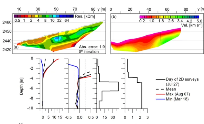
A boundary which reflects the characteristic sharp increase in both resistivity andP-wave velocity at the transition from unfrozen to frozen subsurface conditions can be obtained through the complete profiles at Nair rock glacier (Fig. 3a, b). Corresponding values for this boundary are around 7 km in the ERT profile and 2 km s−1in the SRT profile, respectively. At the position of the borehole, the boundary reaches a depth of 4 m, which is not in accordance with the depth at which the temperature profile from the day of the geophysical measure-ments (daily means) undercuts the 0◦C line (Fig. 3c). How-ever, values from the temperature sensors installed between depths of 3 and 5 m vary between−0.07 and−0.19◦C. This means that the difference from the freezing point is below the accuracy range of the sensors (±0.25◦C). Year-round tem-perature logging (see exemplary plots in Fig. 3c) shows that values of daily mean temperatures are consistently negative below a depth of 3 m, but only the sensors at 9 and 10 m depth show values that are consistently lower than−0.25◦C and hence confirm permafrost conditions. The upslope part of the profiles, where the geophysical profiles are overlap-ping (Y =10–25 m), represents the steep talus cone at the root zone of the rock glacier. Active layer thickness in this part is 2 m. Resistivity values are around 4 km in the un-frozen active layer and vary between 7 and 20 km in the frozen layer. The latter values are considerably lower than the maximum values of the ERT model, which are in the range of several hundred km in an area that is not included in the SRT profile. Only the SRT model, not the shallower ERT model, shows a second boundary at a depth of 12 m, where
disap-Figure 3.Comparative analysis of(a)2-D ERT profile,(b)2-D SRT profile and(c)1-D temperature, resistivity andP-wave velocity profiles at Nair rock glacier. Profiles of resistivity andP-wave velocity are extracted from the tomograms above at the marked borehole position (black line).
Figure 4.Comparative analysis of(a)2-D ERT profile,(b)2-D SRT profile and(c)1-D temperature, resistivity andP-wave velocity profiles at Uertsch rock glacier. Profiles of resistivity andP-wave velocity are extracted from the tomograms above at the marked borehole position (black line).
pears at Y=36 m. The dip angle of this boundary is much steeper than the slope angle of the rock glacier surface at this position. It therefore likely represents the depth of bedrock. The permafrost layer is shaped in a slightly wavy form in both models, which shows an undulating frost table topogra-phy. The courses of this boundary are not fully synchronous between the models, but this variation can be explained by the small parallel shift between the survey lines (Fig. 1d).
4.1.2 Uertsch rock glacier
a depth of 4 m, a sharp increase of resistivity and P-wave velocity can be observed. The vertical temperature profile (daily means) of the borehole from the day of the geophys-ical surveys, reaches 0◦C at the same depth and shows that the detected boundary represents the frost table. Results from year-round temperature logging at the borehole (see exem-plary plots in Fig. 4c) show that down from a depth of 4 m to the end of the thermistor chain, maximum daily mean tem-perature values remain between 0 and−0.18◦C. This repre-sents permanently frozen conditions but is within the accu-racy range of the sensors. In the permafrost layer of the ERT models, resistivity values are between 8 and 39 km. These values can be linked to strong variations of ice content, which range between ice-cemented and ice-supersaturated condi-tions (Ikeda and Matsuoka, 2006). P-wave velocity values of this layer are between 2 and 3.2 km s−1. An area of max-imum high P-wave velocity and maximum high resistivity values, slightly shifted upslope in the SRT profile, is visible around the borehole location. Within the ERT profile, the de-tected permafrost layer ends at a depth of 11 m, where resis-tivity values decrease again. However, low model resolution values in the bottom part of the model (not shown) indicate that this lower boundary is not necessarily constrained by the measured data. P-wave velocity values in the SRT section show a further increase with depth below the lower end of the thermistor chain, which indicates that the frozen layer is un-derlain by unfrozen material with a high level of compaction. As for the ERT profile, it must be noted that data coverage is low in this deeper part of the model. Following the profile in a downslope direction, the layer of highP-wave velocity sharply descends in the SRT model betweenY =45 m and
Y =19 m. This coincides with a decrease of resistivity val-ues to below 5 km and therefore likely represents unfrozen conditions over the complete depth in this part of the profile. The position of this unfrozen part corresponds to the end of the surface ridge structure on which the borehole is placed. In the further downslope part of the profile, the detected struc-tures resemble again those from the upslope part. Near the surface, low resistivity and low P-wave velocity values in-dicate an ALT of 6 m, which is larger than the ALT of the upslope part.
4.2 3-D subsurface models 4.2.1 Nair rock glacier
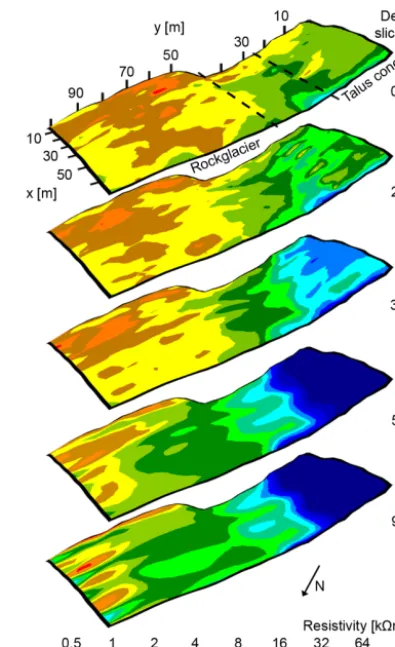
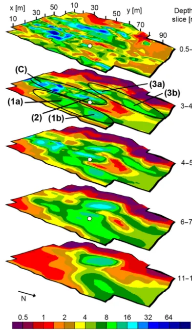
The 3-D model of subsurface resistivity distribution at Nair rock glacier (Fig. 5) shows a strong and stepwise decrease of resistivity values in y direction. The range of modelled re-sistivity values spans from 420 km in the part of the model which corresponds to the talus cone (see Fig. 5, model slice 0.5–1 m) to<1 km in the shallow subsurface of the downs-lope part of the model. Variations inxdirection are less pro-nounced and only show a slight increase of resistivity values
Figure 5.Selected depth slices of the quasi-3-D ERI model for Nair.
from the margin of the rock glacier towards the centre of the rock glacier.
The highest resistivity values aggregate in a 15–25 m long and 40 m wide structure where values between 200 and 400 km in its central part indicate a frozen state. It is over-lain by a 2 m thick layer of lower resistivity values, which vary between 4 and 8 km, and is therefore regarded as the unfrozen active layer. The structure of high resistivity is not shaped homogeneously but narrows slightly along thexaxis towards the blanked out part fromY =42 m to Y=30 m. The vertical extent of the structure exceeds the maximum depth of the model (15 m).
Figure 6. Selected depth slices of the quasi-3-D ERI model for Uertsch_01. Numbers refer to structures described in the text.
in the upper layers are also reduced in this part of the model and vary between 4 and 6 km, which corresponds to similar observations from the 2-D models.
The adjacent part, which corresponds to the main part of the rock glacier, generally shows much lower resistivity val-ues. Like the upslope parts of the model, it can be divided vertically into two layers. An upper layer with values from 1 to 3 km can be delimited from deeper parts of the model where resistivity values vary between 7 and 16 km. Iny di-rection, the boundary between the two layers is descending to a vertical difference of 4 m. This forms a wedge-shaped outline of the high-resistivity layer which penetrates into the rock glacier from the talus cone.
4.2.2 Uertsch rock glacier
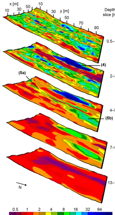
The resistivity model of the lower part of Uertsch rock glacier (Uertsch_01, Fig. 6) shows a heterogeneous pattern of small units. Extraordinary low resistivity values (up to 1.5 km) aggregate in a 10 m wide curved structure in the western part of the model. The areas of the model which show high re-sistivity values can be divided into several tongue-shaped
structures which root in a common zone (marked as (C) in Fig. 6). These structures (named (1) to (3) in the follow-ing, as marked in Fig. 6) can be delimited by extrapolating the threshold value for frozen and unfrozen conditions which was gained from the comparison of geophysical and temper-ature data (the rock glacier is rather homogenous regarding debris size composition). Down to a depth of 6 m, three of those structures are visible atX=12 m (1a, b),X=24 m (2) andX=38 m (3a, b). They are outlined by a band of lower resistivity values. Below a model depth of 6 m, the bound-aries between the tongue-shaped structures vanish, but some parts of the high-resistivity structures remain.
The first of the three structures is 60 m long and reaches a depth of 7 m in the upslope part (1a). In the downslope part (1b), the lower boundary could not be delimited within the model. Resistivity values vary between 7 and 14 km. The layer above this structure is highly variable in thickness. The second structure (2) is about 70 m long and 10 m wide. This structure is penetrated by the borehole as marked in Fig. 6. High resistivity values of up to 30 km aggregate in a layer of 6–8 m thickness. A shallow covering layer of low resis-tivity values exists only partly and shows values of up to 1.5 km. Below the layer of high resistivity, values decrease again. Resistivity values of around 1–3 km are reached in the front of the structure, where a prominent U-shaped patch of lower resistivity values is visible (Fig. 6, depth slices 3–4 and 4–5 m). The third area of high resistivity values is 70 m long and reaches to the northern boundary of the model. The upslope part of the structure (3a) can be obtained in the first model slice, while the downslope part (3b) can be obtained below a depth of 3 m underneath a layer of resistivity values of around 5 km. A lower boundary of the structure could not be delimited within the model boundaries in the upslope part, while the downslope part can be detected down to a depth of 9 m (no depth slice displayed).
The resistivity model of the upper part of Uertsch rock glacier (Uertsch_02, Fig. 7) directly follows the Uertsch_01 model in an upslope direction (see Figs. 1e, 2d). One dom-inant high-resistivity anomaly occurs at the central western part of the model (4) (see Fig. 7 for structures (4) and (5)). It reaches resistivity values from 35 to 250 km. While the upslope part of the structure partly occurs directly below the surface in the first model slice, the downslope part is only vis-ible down from a depth of 2 m where the structure reaches its maximum spatial extent. It remains spatially nearly constant down to a depth of 5 m and decreases in extent and resistivity further downwards.
Figure 7. Selected depth slices of the quasi-3-D ERI model for Uertsch_02. Numbers refer to structures described in the text.
of the Uertsch_02 model, the structure displays values from 7 to 18 km. At a depth of 6 m, it loses an elongated segment (5a) and is reduced in extent to an area of 14 m×30 m. It is detectable down to a depth of 11 m.
The described resistivity distribution clearly reflects the observed surface morphology (see Fig. 2d for morphological structures). It shows high resistivity values within the arcuate (rock glacier snout) and longitudinal ridges (upslope part of the rock glacier) and low resistivity values below the inter-rupting furrows and surface depressions.
5 Discussion
5.1 Methodological aspects
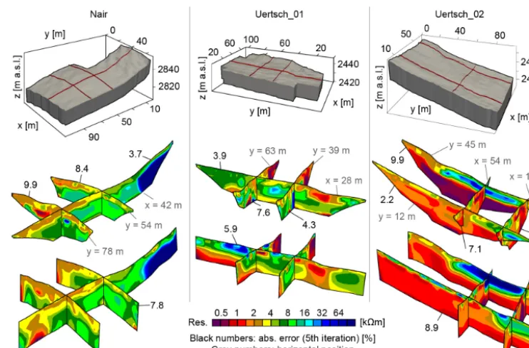
A comparison between independently inverted 2-D models and corresponding 2-D slices of the 3-D models (Fig. 8) shows differences between the results of both approaches.
This affects the modelled resistivity values as well as the depths of the detected structures. At Nair rock glacier, re-sistivity values in the centre of the longitudinal profile (be-tween the perpendicular profiles) are be(be-tween 12 and 16 km in the 2-D model while they are between 8 and 12 km in the 3-D model. Greater differences are shown in the ups-lope part of the longitudinal profile of Uertsch_01. Around
Y=90 m, the 3-D model shows a high-resistivity structure which is displayed with much lower resistivity values by the independently inverted 2-D data. The high-resistivity struc-ture in the Uertsch_02 model (referred to as (4) in Fig. 7) shows a shallow active layer in the results of the 2-D ap-proach, while it appears directly below the surface in the 3-D model. Structures detected by the 3-3-D approach are more smoothly shaped than the same structures detected by the 2-D approach, which is likely the result of diagonal filters and interpolation effects.
The quality of quasi-3-D ERI models is influenced by the separation of the survey grid lines. In our investigation, the chosen value of twice the along-line electrode separation as distance between theY lines of all survey grids provides an adequate data coverage for investigations of the shallow sub-surface (Gharibi and Bentley, 2005). The separation factor of
Xlines was adjusted due to site-specific reasons, like deep snow fields or topographical obstacles and ranges between a factor of 3 and 6 of the along-line electrode spacing. How-ever, this is still assumed to be sufficient as the application of perpendicular grid lines is not a mandatory requirement for 3-D data acquisition but useful for the delimitation of small-scale structures orthogonal to the survey line direction (Loke et al., 2013; Rödder and Kneisel, 2012; Chambers et al., 2002). Despite the known limitations of the DipDip elec-trode array under rough surface conditions (rather low sig-nal strength), its application as a basic electrode array in this study provided very good results. This was likely promoted by the pebbly debris material, which improved the coupling of the electrodes to the ground.
Figure 8.Comparison between independently inverted 2-D (central row) and 3-D (lower row) models. Upper row shows model representa-tions as blocks and posirepresenta-tions of the selected slices.
ERT surveys show good structural accordance and validate the chosen approach.
The detected structures from our geoelectrical investiga-tions of Nair rock glacier broadly resemble the structures which were detected by Ikeda and Matsuoka (2006), who performed a single 2-D ERT survey on the same rock glacier. The P-wave velocity values from their study for a two-layered subsurface (0.34 and 2.9 km s−1) were also broadly reproduced in our study. However, they observed an ALT of 2.2–2.4 m, which is lower than what we observed in our re-sults. This is likely caused by differences in the methodolog-ical approach or in the acquisition geometry. However, the impact of atmospheric warming during the last decade is also conceivable.
5.2 Range of resistivity values
For most parts of the presented rock glacier models, the range of resistivity values for frozen conditions is rather low com-pared to other rock glacier sites (Seppi et al., 2015; Dusik et al., 2015; Kneisel, 2010b; Hilbich et al., 2009; Maurer and Hauck, 2007) and is closer to those of landforms in fine-grained environments (Lewkowicz et al., 2011; Farbrot et al., 2007; Kneisel et al., 2007; Ross et al., 2007). Never-theless, borehole temperature measurements and compara-tive SRT surveys presented in this study indicate the occur-rence of permafrost, althoughP-wave velocity values are in the lowermost range for frozen ground (see compilation of Draebing, 2016). The detected threshold values for a frozen state of around 7 km at Nair rock glacier and around 8 km
at Uertsch rock glacier are plausible for the sites as Ikeda and Matsuoka (2006) found similar values for frozen con-ditions at a similar rock glacier by a comparison between direct observations in a pit and ERT. However, the extrap-olation of a single threshold value on a whole rock glacier can be problematic due to variations of grain size and poros-ity. We think that the extrapolation is suitable at the investi-gated sites, as such variations are not visible on the surface. The low level of resistivity values at the investigated sites can be explained by the small grain size of the debris mate-rial, which is known to show much lower resistivity values in a frozen state than ice-bearing bouldery materials. This is caused by the physical properties of fine materials, which can store a relatively high amount of liquid water at temperatures close to the melting point or even at sub-zero temperatures, resulting in the observed low resistivity values (e.g. Schnei-der et al., 2013). Additionally, the lower pore space volume can generally lower the ground ice volume, which can de-velop by freezing of unconfined water (Scapozza et al., 2011; Vonder Mühll et al., 2000). The non-crystalline origin of the talus material can be listed as another factor which influ-ences the local resistivity regime (Etzelmüller et al., 2006). A high proportion of unfrozen water can also be a reason for the mismatch between the observed frost table depths in the vertical profiles of resistivity,P-wave velocity and temper-ature at Nair rock glacier (Fig. 3c). As the geophysical ap-proaches are affected by material properties and not directly by temperature, the characteristic increase of resistivity and
ob-served sub-zero temperatures (Pogliotti et al., 2015; Hauck, 2002). However, sensor accuracy must also be taken into ac-count. Results from ERT and SRT at Uertsch borehole do not show this mismatch phenomenon. This might be linked to an unhindered drain of unconfined water into the adjacent unfrozen part of the transect.
5.3 Structure of Nair rock glacier
Ice content distribution at Nair rock glacier is probably de-termined by an ice patch of sedimentary origin, buried under the steep talus cone. This is indicated by resistivity values of up to 420 km which display highly ice-supersaturated con-ditions. The occurrence of such structures in the root zone of rock glaciers is a well-known phenomenon which devel-ops from buried snow banks or ice patches which were in-corporated into the subsurface, e.g. by rockfall (Monnier et al., 2011; Lugon et al., 2004; Isaksen et al., 2000; Haeberli and Vonder Mühll, 1996). A high geomorphological activ-ity is present at Nair rock glacier where frequent rockfall events were observed during several field campaigns. The sharp drop in resistivity values to 20 km shows that a clear distinction between the embedded snow bank and the adja-cent part is present. This may indicate a relatively young age of incorporation on timescales of landform development, as this contrast would probably diminish through time. A qual-itatively similar drop of resistivity values was observed by Ribolini et al. (2010) at Schiantala rock glacier (French Mar-itime Alps), where it separates an area of debris-covered sed-imentary ice and an area of typical permafrost ice at the mar-gin of an LIA glaciation. However, linking the incorporation of sedimentary ice into Nair rock glacier to the end of LIA, for which a glaciation is displayed on ancient maps (Coaz and Leuzinger, 1878), is speculative. The occurrence of ice of sedimentary origin below the talus cone is also an ade-quate interpretation for the downslope following part of Nair rock glacier which shows resistivity values typical for con-gelation ice and a decrease from 20 to 12 km.
In this part of the rock glacier, the ability of the pebbly ma-terial to store water and to reduce the speed of runoff (Ikeda et al., 2008) supports the refreezing of the meltwater from the embedded sedimentary ice. This results in a gradual decrease of ice content in a downslope direction and towards the lat-eral margin of the rock glacier, which is less affected by melt-water flow than the main part of the rock glacier. Thus, it can explain the observed stepwise increase of ALT and forms the wedge-shaped structure. If we consider the described pro-cesses as a current phenomenon, the ice-free parts at Nair rock glacier are equal to the permafrost-free parts and vice versa. Stable ground ice conditions at the rock glacier are in-dicated by the gradual shape of the continuous frost table, the generally permafrost-favourable conditions according to the Alpine Permafrost Index Map (Boeckli et al., 2012) and the authors’ own year-round measurements of ground surface temperatures (not shown).
5.4 Structure of Uertsch rock glacier
The observed resistivity variations of the Uertsch rock glacier models indicate variations in ice content and show that dif-ferent processes were involved in rock glacier development. The investigated part of the rock glacier lacks a continuous frost table and the strongly varying ALT indicates a disturbed development. It likely reflects a disequilibrium between the modern environmental conditions and those at the time of ground ice formation.
The ice-free and hence probably unfrozen ridge at the western edge of the rock glacier (extension of the lateral moraine) seems to be unconnected to the more differenti-ated central part. The observed lateral moraine and the sur-face ice patch suggest that interactions between glacial and periglacial processes occurred, like they were assumed for multiple other rock glaciers (Monnier et al., 2011; Ribolini et al., 2010; Berger et al., 2004; Lugon et al., 2004). Glaciation during LIA, as illustrated on an ancient topographical map from the 1870s, was only slightly more extensive than the recent surface ice patch and remained upslope of the today ridge-affected part (see Fig. 2c; Coaz and Leuzinger, 1878). However, like Monnier et al. (2013) pointed out for Sachette rock glacier (French Alps), one of the several other glacier advances during Holocene could have overridden the rock glacier.
The occurrence of buried ice of sedimentary origin is con-ceivable only for the well-defined structure in the central western part of Uertsch rock glacier (Uertsch_02 model), which corresponds to the presumably glacial depression. Next to a surface snow field which existed during the days of the 3-D survey within this depression, maximum resistiv-ity values were detected (250 km). Although this is still not in the range of sedimentary ice which typically reaches up to several Mm (Haeberli and Vonder Mühll, 1996), a sub-surface formation of congelation ice by refreezing meltwater from sedimentary surface ice or an alteration of remnant sed-imentary ice by multiple freeze–thaw cycles seems possible, especially in the case of a former glaciation. The occurrence of buried ice of glacial origin within the rock glacier snout, as also frequently observed at other sites, can be excluded by the range of the modelled resistivity values (<70 km), which indicates distinct patches of congelation ice within the ridges by the three tongue-shaped structures of high resistivity val-ues. A similarly shaped elongated geometry of frozen struc-tures was mapped in the Dolomites by Seppi et al. (2015).
overthrust-ing lobes, as generally presented by Kääb and Weber (2004), fits well to the observations. Ridge formation is assumed to induce a local enrichment of ice content through a thicken-ing of ice-saturated layers (Ikeda and Matsuoka, 2006) and can therefore explain the relatively high ice content within the transverse parts of the arcuate ridges in contrast to the lower ice content of the upslope longitudinal ridges. A patchy occurrence of relatively high ice content within the ridges may also explain the low variation of borehole temperatures around the freezing point as much thermal energy will likely be lost by phase transitions of water. A thickening of the ac-tive layer as described by Haeberli and Vonder Mühll (1996) could only be detected in the lowermost part of the ridges where the deformation is strongest. The upslope central part of the rock glacier, where ridges are shaped in longitudi-nal direction and show resistivity values from 8 to 20 km, lacks this thickening, likely due to a reduced dynamic form-ing. Regarding again the model of overthrusting processes, Kääb and Weber (2004) presumed that those lateral ridges are the result of ridge deformation by a decrease in speed at the margins of the flow area. This former marginal position of the longitudinal ridges supports the concept of a succes-sive rock glacier development. We assume that ridge forma-tion at Uertsch rock glacier is connected to tongue-shaped areas of creep activity on the rock glacier surface. The lower resistivity values of the extensive flow structures are likely caused by freezing of ionically enriched water at the per-mafrost base (Haeberli and Vonder Mühll, 1996). However, a glacial formation of the ridges, e.g. as observed by Monnier et al. (2011) at Thabor rock glacier, cannot be excluded be-cause a general influence of surface ice on the formation of Uertsch rock glacier is obvious.
6 Conclusions
The application of quasi-3-D ERI enables the detection and mapping of permafrost conditions in a spatially extensive way. At Uertsch rock glacier, the approach showed its value for the delimitation of several small-scale frozen structures within heterogeneous subsurface conditions. The rather ho-mogenous subsurface layering at Nair rock glacier excludes the occurrence of major structural anomalies and shows an undulating frost table topography as well as a gradually decreasing ice content. An excellent data quality was pro-moted by the pebbly grain size of the investigated rock glaciers and permitted the extensive application of DipDip electrode array. However, due to the specific conditions at pebbly investigation sites, concerning e.g. the range of resis-tivity values and the influence of grain size on the occurring processes, results should be extrapolated to bouldery rock glaciers only carefully. Inversion characteristics and addi-tionally performed comparative surveys indicate reliable sults and emphasise the suitability of the approach. Our re-sults show that the following subsurface characteristics and
their small-scale spatial variations can be derived from quasi-3-D ERI and interpreted in combination with geomorpholog-ical observations from the investigated rock glaciers:
– Quasi-3-D ERI results in combination with the observed surface ridge structures show that areas of compres-sional and extencompres-sional flow occur in close proximity and indicate a successive rock glacier development.
– Buried ice of sedimentary origin is a crucial factor for rock glacier development as related processes (e.g. meltwater flow) can influence ground ice content distri-bution and reflect past glacier–permafrost interactions.
– Meltwater can strongly increase ground ice content in downslope and less inclined parts of rock glaciers and changes its distribution to a gradual decrease which fol-lows the observed rock glacier topography and results in a wedge-shaped outline of the permafrost body.
– Mapping frost table topography and consistency allow us to infer the occurrence of shaping processes and hence to assess whether a state of equilibrium or dis-equilibrium to modern environmental conditions exists. To further improve our understanding of landform devel-opment, the additional application of GPR and the set-up of a denser network of SRT profiles are advised as these ap-proaches are preferably used for the detection of layer bound-aries. The presented resistivity mapping further allows an overlay of resistivity distribution with mapping of surface flow velocity and subsurface porosity. This might be a next step towards an identification of surface–subsurface process interactions.
7 Data availability
Geophysical data are available upon request from the au-thors.
Acknowledgements. The authors gratefully acknowledge the German Research Foundation (DFG) for financial support (KN542/13-1) and the municipalities of Celerina and Bergün for the permission to use their access roads. Thanks to Danilo Fries and Carina Selbach for their assistance in the field. We would also like to thank the editor, Christian Hauck, and two anonymous reviewers for their constructive comments. This publication was funded by the German Research Foundation (DFG) and the University of Würzburg in the funding programme Open Access Publishing.
Edited by: C. Hauck
References
Berger, J., Krainer, K., and Mostler, W.: Dynamics of an active rock glacier (Ötztal Alps, Austria), Quarternary Res., 62, 233–242, doi:10.1016/j.yqres.2004.07.002, 2004.
Boeckli, L., Brenning, A., Gruber, S., and Noetzli, J.: Permafrost distribution in the European Alps: calculation and evaluation of an index map and summary statistics, The Cryosphere, 6, 807– 820, doi:10.5194/tc-6-807-2012, 2012.
Chambers, J. E., Ogilvy, R. D., Kuras, O., Cripps, J., and Mel-drum, P. I.: 3D electrical imaging of known targets at a con-trolled environmental test site, Environ. Geol., 41, 690–704, doi:10.1007/s00254-001-0452-4, 2002.
Coaz, J. W. F. and Leuzinger, R.: Bevers, Eidg. Stabsbureau, Bern, 1878.
Coaz, J. W. F., Leuzinger, R., and Held, L.: St. Moritz, Eidg. Stab-sbureau [i.e. Eidg. Landestopographie], Bern, Nachträge 1917, 1925.
Coaz, J. W. F., Leuzinger, R., and Held, L.: St. Moritz, Eidg. Lan-destopographie, Bern, Nachträge 1944, 1946.
Draebing, D.: Application of refraction seismics in alpine per-mafrost studies: A review, Earth-Sci. Rev., 155, 136–152, 2016. Dusik, J.-M., Leopold, M., Heckmann, T., Haas, F., Hilger, L.,
Morche, D., Neugirg, F., and Becht, M.: Influence of glacier ad-vance on the development of the multipart Riffeltal rock glacier, Central Austrian Alps, Earth Surf. Proc. Land., 40, 965–980, doi:10.1002/esp.3695, 2015.
Etzelmüller, B., Heggem, E. S. F., Sharkhuu, N., Frauenfelder, R., Kääb, A., and Goulden, C.: Mountain permafrost distri-bution modelling using a multi-criteria approach in the Hövs-göl area, northern Mongolia, Permafrost Periglac., 17, 91–104, doi:10.1002/ppp.554, 2006.
Farbrot, H., Etzelmüller, B., Schuler, T. V., Guðmundsson, Á., Eiken, T., Humlum, O., and Björnsson, H.: Thermal characteristics and impact of climate change on moun-tain permafrost in Iceland, J. Geophys. Res., 112, F03S90, doi:10.1029/2006JF000541, 2007.
Frehner, M., Ling, A. H. M., and Gärtner-Roer, I.: Furrow-and-Ridge Morphology on Rockglaciers Explained by Gravity-Driven Buckle Folding: A Case Study From the Murtèl Rockglacier (Switzerland), Permafrost Periglac., 26, 57–66, doi:10.1002/ppp.1831, 2015.
Geometrics: SeisImager/2D™Manual, Version 3.3, 2009. Gharibi, M. and Bentley, L. R.: Resolution of 3-D Electrical
Resis-tivity Images from Inversions of 2-D Orthogonal Lines, J. En-viron. Eng. Geoph., 10, 339–349, doi:10.2113/JEEG10.4.339, 2005.
Haeberli, W. and Vonder Mühll, D. S.: On the characteristics and possible origins of ice in rock glacier permafrost, Z. Geomor-phol., Suppl.-Bd. 104, 43–57, 1996.
Haeberli, W., Hallet, B., Arenson, L. U., Elconin, R., Hum-lum, O., Kääb, A., Kaufmann, V., Ladanyi, B., Matsuoka, N., Springman, S. M., and Vonder Mühll, D. S.: Permafrost creep and rock glacier dynamics, Permafrost Periglac., 17, 189–214, doi:10.1002/ppp.561, 2006.
Hanson, S. and Hoelzle, M.: The thermal regime of the active layer at the Murtèl rock glacier based on data from 2002, Permafrost Periglac., 15, 273–282, doi:10.1002/ppp.499, 2004.
Harris, C., Arenson, L. U., Christiansen, H. H., Etzelmüller, B., Frauenfelder, R., Gruber, S., Haeberli, W., Hauck, C.,
Hoel-zle, M., Humlum, O., Isaksen, K., Kääb, A., Kern-Lütschg, M. A., Lehning, M., Matsuoka, N., Murton, J. B., Nötzli, J., Phillips, M., Ross, N., Seppälä, M., Springman, S. M., and Vonder Mühll, D. S.: Permafrost and climate in Eu-rope: Monitoring and modelling thermal, geomorphological and geotechnical responses, Earth-Sci. Rev., 92, 117–171, doi:10.1016/j.earscirev.2008.12.002, 2009.
Harris, S. A. and Pedersen, D. E.: Thermal regimes beneath coarse blocky materials, Permafrost Periglac., 9, 107–120, doi:10.1002/(SICI)1099-1530(199804/06)9:2<107:AID-PPP277>3.0.CO;2-G, 1998.
Hauck, C.: Frozen ground monitoring using DC resis-tivity tomography, Geophys. Res. Lett., 29, 12-1–12-4, doi:10.1029/2002GL014995, 2002.
Hauck, C.: New Concepts in Geophysical Surveying and Data Inter-pretation for Permafrost Terrain, Permafrost Periglac., 24, 131– 137, doi:10.1002/ppp.1774, 2013.
Hauck, C., Böttcher, M., and Maurer, H.: A new model for esti-mating subsurface ice content based on combined electrical and seismic data sets, The Cryosphere, 5, 453–468, doi:10.5194/tc-5-453-2011, 2011.
Hausmann, H., Krainer, K., Brückl, E., and Ullrich, C.: Internal structure, ice content and dynamics of Ölgrube and Kaiserberg rock glaciers (Ötztal Alps, Austria) de-termined from geophys-ical surveys, Austrian Journal of Earth Sciences, 105, 12–31, 2012.
Hilbich, C., Marescot, L., Hauck, C., Loke, M. H., and Mäusbacher, R.: Applicability of electrical resistivity tomography monitoring to coarse blocky and ice-rich permafrost landforms, Permafrost Periglac., 20, 269–284, doi:10.1002/ppp.652, 2009.
Hoelzle, M., Wegmann, M., and Krummenacher, B.: Miniature tem-perature dataloggers for mapping and monitoring of permafrost in high mountain areas: First experience from the Swiss Alps, Permafrost Periglac., 10, 113–124, doi:10.1002/(SICI)1099-1530(199904/06)10:2<113:AID-PPP317>3.0.CO;2-A, 1999. Ikeda, A.: Combination of conventional geophysical methods for
sounding the composition of rock glaciers in the Swiss Alps, Per-mafrost Periglac., 17, 35–48, doi:10.1002/ppp.550, 2006. Ikeda, A. and Matsuoka, N.: Pebbly versus bouldery rock glaciers:
Morphology, structure and processes, Geomorphology, 73, 279– 296, doi:10.1016/j.geomorph.2005.07.015, 2006.
Ikeda, A., Matsuoka, N., and Kääb, A.: Fast deformation of peren-nially frozen debris in a warm rock glacier in the Swiss Alps: An effect of liquid water, J. Geophys. Res., 113, F01021, doi:10.1029/2007JF000859, 2008.
Isaksen, K., Ødegård, R. S., Eiken, T., and Sollid, J. L.: Com-position, flow and development of two tongue-shaped rock glaciers in the permafrost of Svalbard, Permafrost Periglac., 11, 241–257, doi:10.1002/1099-1530(200007/09)11:3<241:AID-PPP358>3.0.CO;2-A, 2000.
Kääb, A. and Weber, M.: Development of transverse ridges on rock glaciers: Field measurements and laboratory experiments, Per-mafrost Periglac., 15, 379–391, doi:10.1002/ppp.506, 2004. Kääb, A., Frauenfelder, R., and Roer, I.: On the response of
rock-glacier creep to surface temperature increase, Global Planet. Change, 56, 172–187, doi:10.1016/j.gloplacha.2006.07.005, 2007.
Hochge-birgen (GMK Hochgebirge), Geographische Gesellschaft, Trier, Trierer geographische Studien, 18, 24 pp., 1998.
Kneisel, C.: Frozen ground conditions in a subarctic mountain environment, Northern Sweden, Geomorphology, 118, 80–92, doi:10.1016/j.geomorph.2009.12.010, 2010a.
Kneisel, C.: The nature and dynamics of frozen ground in alpine and subarctic periglacial environments, Holocene, 20, 423–445, doi:10.1177/0959683609353432, 2010b.
Kneisel, C. and Kääb, A.: Mountain permafrost dynamics within a recently exposed glacier forefield inferred by a combined ge-omorphological, geophysical and photogrammetrical approach, Earth Surf. Proc. Land., 32, 1797–1810, doi:10.1002/esp.1488, 2007.
Kneisel, C., Sæmundsson, Þ., and Beylich, A. A.: Reconnaissance Surveys Of Contemporary Permafrost Environments In Cen-tral Iceland Using Geoelectrical Methods: Implications For Per-mafrost Degradation And Sediment Fluxes, Geogr. Ann. A, 89, 41–50, doi:10.1111/j.1468-0459.2007.00306.x, 2007.
Kneisel, C., Hauck, C., Fortier, R., and Moorman, B.: Advances in geophysical methods for permafrost investigations, Permafrost Periglac., 19, 157–178, doi:10.1002/ppp.616, 2008.
Kneisel, C., Emmert, A., and Kästl, J.: Application of 3D elec-trical resistivity imaging for mapping frozen ground conditions exemplified by three case studies, Geomorphology, 210, 71–82, doi:10.1016/j.geomorph.2013.12.022, 2014.
Krainer, K., Mussner, L., Behm, M., and Hausmann, H.: Multi-discipliary investigation of an active rock glacier in the Sella Group (Dolomites; Northern Italy), Austrian Journal of Earth Sciences, 105, 48–62, 2012.
Lambiel, C. and Pieracci, K.: Permafrost distribution in talus slopes located within the alpine periglacial belt, Swiss Alps, Permafrost Periglac., 19, 293–304, doi:10.1002/ppp.624, 2008.
Langston, G., Bentley, L. R., Hayashi, M., McClymont, A., and Pidlisecky, A.: Internal structure and hydrological functions of an alpine proglacial moraine, Hydrol. Process., 2967–2982, doi:10.1002/hyp.8144, 2011.
Lewkowicz, A. G., Etzelmüller, B., and Smith, S. L.: Charac-teristics of Discontinuous Permafrost based on Ground Tem-perature Measurements and Electrical Resistivity Tomography, Southern Yukon, Canada, Permafrost Periglac., 22, 320–342, doi:10.1002/ppp.703, 2011.
Loke, M. H.: Tutorial: 2D and 3D electrical imaging surveys, Geotomo Software, Malaysia, 2014.
Loke, M. H.: Rapid 3-D Resistivity & IP inversion using the least-squares method (For 3-D surveys using the pole-pole, pole-dipole-pole, dipole-dipole-pole, rectangular, Wenner, Wenner-Schlumberger and non-conventional arrays) On land, aquatic, cross-borehole and time-lapse surveys, Geotomo Software, Malaysia, 2015.
Loke, M. H. and Barker, R. D.: Practical techniques for 3D resis-tivity surveys and data inversion1, Geophys. Prospect., 44, 499– 523, doi:10.1111/j.1365-2478.1996.tb00162.x, 1996.
Loke, M. H., Chambers, J. E., Rucker, D. F., Kuras, O., and Wilkinson, P. B.: Recent developments in the direct-current geo-electrical imaging method, J. Appl. Geophys., 95, 135–156, doi:10.1016/j.jappgeo.2013.02.017, 2013.
Luetschg, M., Stoeckli, V., Lehning, M., Haeberli, W., and Am-mann, W.: Temperatures in two boreholes at Flüela Pass, Eastern Swiss Alps: The effect of snow redistribution on permafrost
dis-tribution patterns in high mountain areas, Permafrost Periglac., 15, 283–297, doi:10.1002/ppp.500, 2004.
Luetschg, M., Lehning, M., and Haeberli, W.: A sensitivity study of factors influencing warm/thin permafrost in the Swiss Alps, J. Glaciol., 54, 696–704, doi:10.3189/002214308786570881, 2008.
Lugon, R., Delaloye, R., Serrano, E., Reynard, E., Lambiel, C., and González-Trueba, J. J.: Permafrost and Little Ice Age glacier re-lationships, Posets Massif, Central Pyrenees, Spain, Permafrost Periglac., 15, 207–220, doi:10.1002/ppp.494, 2004.
Matsuoka, N., Ikeda, A., and Date, T.: Morphometric analysis of solifluction lobes and rock glaciers in the Swiss Alps, Permafrost Periglac., 16, 99–113, doi:10.1002/ppp.517, 2005.
Maurer, H. and Hauck, C.: Geophysical imaging of alpine rock glaciers, J. Glaciol., 53, 110–120, doi:10.3189/172756507781833893, 2007.
Monnier, S., Camerlynck, C., Rejiba, F., Kinnard, C., Feuillet, T., and Dhemaied, A.: Structure and genesis of the Thabor rock glacier (Northern French Alps) determined from morphologi-cal and ground-penetrating radar surveys, Geomorphology, 134, 269–279, doi:10.1016/j.geomorph.2011.07.004, 2011.
Monnier, S., Camerlynck, C., Rejiba, F., Kinnard, C., and Galibert, P.-Y.: Evidencing a large body of ice in a rock glacier, Vanoise Massif, Northern French Alps, Geogr. Ann. A, 95, 109–123, doi:10.1111/geoa.12004, 2013.
Musil, M., Maurer, H., Hollinger, K., and Green, A. G.: Internal structure of an alpine rock glacier based on crosshole georadar traveltimes and amplitudes, Geophys. Prospect., 54, 273–285, doi:10.1111/j.1365-2478.2006.00534.x, 2006.
Otto, J. C. and Sass, O.: Comparing geophysical meth-ods for talus slope investigations in the Turtmann valley (Swiss Alps), Geomorphology, 76, 257–272, doi:10.1016/j.geomorph.2005.11.008, 2006.
Otto, J. C., Keuschnig, M., Götz, J., Marbach, M., and Schrott, L.: Detection Of Mountain Permafrost By Combining High Resolu-tion Surface And Subsurface InformaResolu-tion – An Example From The Glatzbach Catchment, Austrian Alps, Geogr. Ann. A, 94, 43–57, doi:10.1111/j.1468-0459.2012.00455.x, 2012.
Pellet, C., Hilbich, C., Marmy, A., and Hauck, C.: Soil moisture data for the validation of permafrost models using direct and indirect measurement approaches at three alpine sites, Front. Earth Sci., 3, 91, doi:10.3389/feart.2015.00091, 2016.
Pogliotti, P., Guglielmin, M., Cremonese, E., Morra di Cella, U., Filippa, G., Pellet, C., and Hauck, C.: Warming permafrost and active layer variability at Cime Bianche, Western European Alps, The Cryosphere, 9, 647–661, doi:10.5194/tc-9-647-2015, 2015. Ribolini, A., Guglielmin, M., Fabre, D., Bodin, X., Marchisio,
M., Sartini, S., Spagnolo, M., and Schoeneich, P.: The inter-nal structure of rock glaciers and recently deglaciated slopes as revealed by geoelectrical tomography: Insights on per-mafrost and recent glacial evolution in the Central and West-ern Alps (Italy–France), QuatWest-ernary Sci. Rev., 29, 507–521, doi:10.1016/j.quascirev.2009.10.008, 2010.
Rödder, T. and Kneisel, C.: Permafrost mapping using quasi-3D re-sistivity imaging, Murtèl, Swiss Alps, Near Surf. Geophys., 10, 117–127, doi:10.3997/1873-0604.2011029, 2012.
Ground-ice Conditions, J. Environ. Eng. Geoph., 12, 113–126, doi:10.2113/JEEG12.1.113, 2007.
Scapozza, C. and Laigre, L.: The contribution of Electrical Resis-tivity Tomography (ERT) in Alpine dynamics geomorphology: case studies from the Swiss Alps?, Géomorphologie, 20, 27–42, 2014.
Scapozza, C., Lambiel, C., Baron, L., Marescot, L., and Reynard, E.: Internal structure and permafrost distribution in two alpine periglacial talus slopes, Valais, Swiss Alps, Geomorphology, 132, 208–221, doi:10.1016/j.geomorph.2011.05.010, 2011. Scherler, M., Hauck, C., Hoelzle, M., and Salzmann, N.:
Mod-eled sensitivity of two alpine permafrost sites to RCM-based climate scenarios, J. Geophys. Res.-Earth, 118, 780–794, doi:10.1002/jgrf.20069, 2013.
Schneider, S., Hoelzle, M., and Hauck, C.: Influence of surface and subsurface heterogeneity on observed borehole temperatures at a mountain permafrost site in the Upper Engadine, Swiss Alps, The Cryosphere, 6, 517–531, doi:10.5194/tc-6-517-2012, 2012. Schneider, S., Daengeli, S., Hauck, C., and Hoelzle, M.: A spatial
and temporal analysis of different periglacial materials by using geoelectrical, seismic and borehole temperature data at Murtèl– Corvatsch, Upper Engadin, Swiss Alps, Geogr. Helv., 68, 265– 280, doi:10.5194/gh-68-265-2013, 2013.
Schrott, L. and Hoffmann, T.: Refraction Seismics, in: Applied Geophysics in Periglacial Environments, Cambridge University Press, 57–80, 2008.
Schrott, L. and Sass, O.: Application of field geophysics in geomorphology: Advances and limitations exem-plified by case studies, Geomorphology, 93, 55–73, doi:10.1016/j.geomorph.2006.12.024, 2008.
Seppi, R., Zanoner, T., Carton, A., Bondesan, A., Francese, R., Carturan, L., Zumiani, M., Giorgi, M., and Ninfo, A.: Cur-rent transition from glacial to periglacial processes in the Dolomites (South-Eastern Alps), Geomorphology, 228, 71–86, doi:10.1016/j.geomorph.2014.08.025, 2015.
Springman, S. M., Arenson, L. U., Yamamoto, Y., Maurer, H., Kos, A., Buchli, T., and Derungs, G.: Multidisciplinary Investigations On Three Rock Glaciers In The Swiss Alps: Legacies And Future Perspectives, Geogr. Ann. A, 94, 215–243, doi:10.1111/j.1468-0459.2012.00464.x, 2012.
Stummer, P., Maurer, H., and Green, A. G.: Experimental design: Electrical resistivity data sets that provide optimum subsurface information, Geophysics, 69, 120–139, doi:10.1190/1.1649381, 2004.
Vonder Mühll, D. S., Hauck, C., and Lehmann, F.: Verifi-cation of geophysical models in Alpine permafrost us-ing borehole information, Ann. Glaciol., 31, 300–306, doi:10.3189/172756400781820057, 2000.