A Combination Method for Averaging OLS and GLS Estimators

(1)

Article

A Combination Method for Averaging OLS and

GLS Estimators

†

Qingfeng Liu1,* and Andrey L. Vasnev2

1 _{Department of Economics, Otaru University of Commerce, Otaru 047-8501, Japan}

2 _{Discipline of Business Analytics, The University of Sydney Business School, The University of Sydney,}

Sydney, NSW 2006, Australia; [email protected] * Correspondence: [email protected]

† The authors thank Okui Ryo, Mototsugu Shintani, Arihiro Yoshimura and the conference participants at the 2014 European Meeting of the Econometric Society and the 2013 Kansai Keiryo Keizaigaku Kenkyukai for their helpful comments. Liu acknowledges financial support from the JSPS Grant-in-Aid for Young Scientists (B) No. 25780148 and JSPS KAKENHI Grant (C) No. JP16K03590 and No. JP19K01582. The authors are grateful to the Editor and two reviewers for their constructive comments.

Received: 6 June 2019; Accepted: 4 September 2019; Published: 9 September 2019

Abstract: To avoid the risk of misspecification between homoscedastic and heteroscedastic models, we propose a combination method based on ordinary least-squares (OLS) and generalized least-squares (GLS) model-averaging estimators. To select optimal weights for the combination, we suggest two information criteria and propose feasible versions that work even when the variance-covariance matrix is unknown. The optimality of the method is proven under some regularity conditions. The results of a Monte Carlo simulation demonstrate that the method is adaptive in the sense that it achieves almost the same estimation accuracy as if the homoscedasticity or heteroscedasticity of the error term were known.

Keywords:model averaging; OLS; GLS; combination method

1. Introduction

Model averaging has been developed as an alternative to model selection. In many situations, model-averaging methods perform better than alternative model-selection methods. The main reason for this is that model selection delivers a pretest estimator that has inferior properties, and its use can be harmful (seeDanilov and Magnus,2004). Yuan and Yang(2005) provided a detailed discussion on the choice between model averaging and model selection. As one of the pioneers of frequentist model averaging,Hansen(2007) proposed Mallows model averaging (MMA) based on the ordinary least-squares (OLS) estimator for linear regression models with homoscedastic errors.Wan et al.(2010) extended the results for non-nested models with homoscedastic errors.Zhao et al.(2018) is the most recent work in this area. For linear regression models with heteroscedastic errors,Hansen and Racine (2012),Liu and Okui(2013) andZhang et al.(2013,2015) proposed model averaging methods that are still based on the OLS estimator, whileLiu et al.(2016) proposed a method based on the generalized least squares estimator (GLS). They demonstrated that their methods are optimal in the sense of Li(1987) for homoscedastic or heteroscedastic models. For model averaging in big datasets,Xie(2017) proposed the use of model screening (before averaging) in order to deal with the large number of candidate models/regressors.

However, all previous papers assumed that it was known whether the errors of the true data-generating process are homoscedastic or heteroscedastic. Due to this assumption, the previous averaging methods were based only on estimators constructed using the same estimation method,

(2)

either OLS or GLS estimators (with different regressor sets). This assumption can be unrealistic in empirical applications. Usually, researchers do not know the structure of the error term; therefore, this assumption leads to possible misspecification. A natural solution is to combine OLS and GLS estimators. Combinations of different methods are routinely used in the applied forecast combination literature. In a recent forecasting competition that included 100,000 series,Makridakis et al.(2018) found that, out of the 17 most accurate methods, 12 were combinations. All combinations used different models/methods varying from simple exponential smoothing models to sophisticated machine-learning algorithms.

We propose a combination method based on OLS and GLS estimators to reduce the risk of misspecification between homoscedastic and heteroscedastic linear models. More precisely, the proposed estimator is a weighted average of mixtures of OLS and GLS estimators. The OLS mixture is constructed using the MMA ofHansen(2007) or the heteroscedasticity-robust Cp(HRCp) model averaging of Liu and Okui(2013). The GLS mixture is constructed using the GLS model averaging (GLSMA) ofLiu et al.(2016).

We propose the use of two criteria, MMA-GLSMA and HRCp-GLSMA, to choose the weight vector for combining estimators. The optimality of the chosen weight vector in the sense ofLi(1987) is investigated. Our method works in situations with an unknown variance-covariance matrix of the error term if an estimate based on the nonparametric method k-nearest neighbours (k-NN) is used. The results of the simulation experiments show that our combination method is adaptive in the sense that it can achieve almost the same estimation accuracy as if the homoscedasticity or heteroscedasticity of the error term was known.

The rest of the paper is organized as follows: In Section2, we describe the theoretical setup and introduce the new combination method with the criteria for choosing the weight vector. In Section3, we investigate the optimality of the proposed criteria. Section4presents the results of the Monte Carlo simulations. Section5concludes the paper, and all proofs are provided in the AppendixA.

2. Method

Suppose that we have an independent random sample of (yi,xi) for i = 1, . . . ,n, where xi= (xi1,xi2, . . . ,)0 is a countably infinite real-valued vector andyi is a real-valued scalar random variable generated from an infinite dimensional linear regression model:

yi = µi+ei,

where:

µi = ∞

∑

j=1

θjxij,

eiis an unobserved error term that can be homoscedastic or heteroscedastic withE(ei|xi) =0,E(e2i) =σ2 andE(e2_i|xi) =σ_i2andθjforj=1, 2,· · · are unknown parameters. We also defineX≡(x1,· · ·,xn),

Y ≡ (y1,· · ·,yn)

0

,µ ≡ (µ1,· · ·,µn)

0

,e ≡ (e1,· · ·,en)

0

and denote the variance-covariance matrix asΩ ≡ Eee0|X =diag(σ₁2,· · ·,σ_n2). We state the theoretical results considering the distributions conditional onXand omit all notations for those conditional onXhereafter.

2.1. Infeasible Combination Estimator and Information Criteria

SupposeΩis known; we have a candidate set ofM1linear models with different numbers of independent variables for OLS estimation and a candidate set of M2linear models with different numbers of independent variables for GLS estimation. Then, we can obtain a set of OLS estimates ˆµolsm ≡

PmYform= 1,· · ·,M1and a set of GLS estimates ˆµglsm ≡ GmYform= 1,· · ·,M2. Therein,Pm =

(3)

and Gm ≡ Xm(X0mΩ−1Xm)−1Xm0 Ω−1 with Xm being the independent variable matrix of the mth regression model for GLS withm = 1,· · ·,M2. In this paper, we only consider the situation with nested models for both OLS and GLS estimators. This means that themth model is nested in the (m+1)th model. Theoretical results may be extended to non-nested candidate models using the approach ofWan et al.(2010). Moreover,M1andM2can be fixed or go to infinity when the sample sizenis increasing.

Based on those OLS and GLS estimates, we construct a combination estimator as follows:

ˆ µ(W) =

M1

∑

m=1

wolsm µˆolsm + M2

∑

m=1

wglsm µˆglsm ,

≡µˆ_ols(W1) +µˆ_gls(W2)

whereW=W₁0,W₂0=w₁ols,· · ·,wols_M₁,w₁gls,· · ·,wgls_M₂ 0

belongs to:

H=nW

W∈[0, 1] M

, I0W=1o,

whereM=M1+M2andIdenote aM×1 vector having all elements equal to one.

In order to reduce the risk of the combination-estimation method proposed above, we need to select a suitable weight vector. To do that, in this subsection, we propose two versions, MMA-GLSMA and HRCp-GLSMA, with infeasible criteria. In the next subsection, we provide their feasible counterparts for the situation with unknownΩvalues.

HRCp-GLSMA: The first information criterion for selecting a weight vector is defined as:

¯

Cn(W) = s21 n

kY−µˆ_ols(W₁∗)k2+2tr(P(W₁∗)Ω) o

(1)

+s2₂

Y−µˆgls(W ∗ 2)

2

+2tr(G(W₂∗)Ω)

(2)

+2s1s2 n

(Y−µˆols(W1∗)) 0

Y−µˆgls(W2∗)

(3)

+tr(P(W₁∗)Ω) +tr(G(W₂∗)Ω)−e0eo, (4)

where s1 ≡ ∑_mM₌₁1 wolsm ,s2 ≡ ∑_mM₌₁2 wglsm ,W₁∗ ≡ W1/s1,W2∗ ≡ W2/s2, P W₁∗ ≡ ∑M_m₌₁1 wolsm Pm and G(W₂∗)≡_∑M2

m=1w

gls m Gm. Note that:

¯

Cn(W) =s21HRCp(W1∗) +s22CIn(W ∗ 2)

+2s1s2 n

Y−µˆgls(W2∗)

+tr(P(W₁∗)Ω) +tr(G(W₂∗)Ω)−e0eo,

where HRCp W₁∗ = Y−µˆols W1∗

2

+2tr P W₁∗

Ω

is the HRCp model-averaging criterion

proposed byLiu and Okui(2013) with the weight vectorW₁∗ andCIn(W ∗ 2) =

Y−µˆgls(W ∗ 2)

2

+ 2tr(G(W₂∗)Ω) is a GLSMA information criterion proposed by Liu et al. (2016) with the weight vectorW₂∗. ¯Ccan be regarded as a combination of the HRCp and the GLSMA. Hence, we call ¯Cthe HRCp-GLSMA-type criterion.

MMA-GLSMA: Second, we propose an MMA-GLSMA-type criterion for weight selection. The infeasible MMA-GLSMA-type criterion is defined as follows:

e

(4)

+2s1s2 n

Y−µˆgls(W2∗)

+σ2tr(P(W₁∗)) +tr(G(W₂∗)Ω)−e

0 eo,

whereCMMA W1∗

=

Y−µˆ_ols W₁∗

2

+2σ2tr P W₁∗is the MMA criterion proposed byHansen (2007) with the weight vectorW₁∗.

Suppose the variance-covariance matrix Ω is known; we can then choose the weight by minimizing the criteria ¯CnorCen, as follows:

¯

W=arg min W∈H

¯ Cn

or

e

W=arg min W∈HCen.

However, since the variance-covariance matrixΩis unknown, ¯Wand ˜Ware infeasible.

2.2. Feasible Combination Estimator and Information Criteria

For a situation with unknown variance, a feasible combination estimator can be constructed using feasible GLS (FGLS) estimators. FGLS estimators and the feasible combination estimator are defined below:

ˆ

µF(W) = M₁

∑

m=1

wolsm µˆolsm + M2

∑

m=1

wglsm µˆmf gls,

≡µˆols(W1) +µˆf gls(W2)

where the FGLS estimator is ˆµmf gls ≡Xm(Xm0 Ωˆ−1Xm)−1X0mΩˆ−1Y. Therein, the estimator ˆΩis based on thek-NN estimator ˇσi2ofLiu et al.(2016).

We propose two feasible counterparts of ¯CnandCe_n. The feasible HRCp-GLSMA-type criterion ¯

CnFis defined as:

¯

CF_n(W) = s2 1

n

2

+2∑n

i=1eˆ2ipii W1∗ o

+s2₂

Y−µˆf gls(W ∗ 2) 2

+2tr GF(W₂∗)Ωˆ

+2s1s2 n

Y−µˆols W1∗ 0

Y−µˆf gls(W2∗)

+tr P W₁∗ _ˆ

Ω

+tr GF_(W∗ 2)Ωˆ

−eˆ0eˆo,

(5)

and the feasible MMA-GLSMA-type criterionCe_nFis defined as:

e

CFn(W) = s21 n

2

+2 ˆσ2tr P W₁∗ o

+s2₂

Y−µˆf gls(W ∗ 2) 2

+2tr GF(W₂∗)Ωˆ

+2s1s2 n

Y−µˆols W1∗ 0

Y−µˆf gls(W2∗)

+σˆ2tr P W₁∗+tr GF(W₂∗)Ωˆ−eˆ0eˆ o

,

(6)

where ˆei denotes the ith element of ˆe ≡ p

n/(n−kL)(I−PL)Y withkL denoting the number of independent variables in the largest OLS model:

GF(W₂∗) = M2

∑

m=1

(5)

PLdenotes the projection matrix of that model, andpiidenotes theithdiagonal element ofP W1∗

. ˜e≡ (I−PL)Y, while ˆσ2≡(n−kL)−1e˜

0 ˜

eis defined as one of the estimators suggested byHansen(2007). ˆ

Ωis calculated by plugging in thek-NN estimator ˇσi2used inLiu et al.(2016).

3. Properties of the Criteria

The following lemma demonstrates the significant fact that the two infeasible criteria proposed above are unbiased estimates of the risk functionR(W)≡E(L(W))plus a constant;L(W)≡ kµ−µˆ(W)k2is the loss function.

Lemma 1. For any real-valued vector W, E(C¯n(W)) = R(W) +c1 and E

e Cn(W)

= R(W) +c2, where c1and c2are constants.

Another useful property is that all criteria are asymptotically optimal in the sense ofLi(1987). Proofs of the asymptotic optimality for all of the above-mentioned criteria can be performed by extending the proofs of Hansen (2007); Liu and Okui (2013); Liu et al.(2016). As an example, we demonstrate the optimality of the feasible MMA-GLSMA case method with the nonparametric estimator ofΩused inLiu et al.(2016).

To do that, we define the feasible loss function and the risk function as follows:

LF(W)≡ µ−µˆ

F_(W) 2

= (µˆF(W)−µ)0(µˆF(W)−µ).

We employ some notations and assumptions fromLiu et al.(2016), reproduced in the Appendix, and add the following additional assumption:

Assumption 1’.As n→∞and kl→∞,

kl+kl q

∑n

j=1b2lj

/ξn→0, whereξn ≡infW∈Hn(N)R(W), kl is the number of regressors used in the regression model for the k-NN estimator and blidenotes the approximation error of that model.

Assumption 1’ guarantees that when the number of regressors used in the regression model (adjusted with the approximation errors of that model) increases with the sample sizen, it increases at a rate slower than the lower bound of the risk across all possible weights. In practice, this assumption requires us to moderate the increase in the number of regressorskl (relative to the sample size) to reduce the approximation errors.

Following Hansen (2007), we restrict the elements of the weighting vector to belong to set

HM(N)≡ {0, 1/N, 2/N, . . . , 1}for some integerN<∞.

Theorem 1. Under Assumption 1’ and Assumptions 1–3, 6, and 10–14 ofLiu et al.(2016), as n→∞, kl→∞, κ→∞and kL/

√

n→0, we have:

LF(W)e infW∈HM(N)L(W)

→p1,

whereWe =arg min_W_∈H M(N)Ce

F n(W).

In other words, as the sample size increases, our method can achieve the infimum of the loss.

4. Simulation Study

(6)

The data-generating process (DGP) is:

yi = µi+ei,

where:

µi =

10,000

∑

j=1

θjxij

fori=1,· · ·,n, withn=50. We used parameterθj =cj−1withjtruncated at 10,000 and a positive

constantc.xi1=1 andxij∼N(0, 1)forj6=1 are independent with respect toi. We conducted three simulations. The first case was a simulation with a homoscedastic error termei∼N(0, 1). The second case was a mild heteroscedastic case with heteroscedastic error termei ∼ N 0,σ_i2, withσi = |xi2|. The third case was a strong heteroscedastic case withσi=x2i2. In all cases,eiwas independent with respect toi. The number of regressors in the largest approximation model or the number of nested models was M =10. Themthmodel contained the firstmregressors, including the constant term. We variedcto change theR2_{of the DGP from 0.1–0.9 with an increment of 0.1.}

We considered two cases of GLSMA with different estimation methods ofσi, one based on the maximum likelihood estimation (MLE), and the other based on the nonparametric methodk-NN. For details of these two cases, seeLiu et al.(2016). Because the true specification ofσi is usually unknown in practice, we misspecifiedσifor GLSMA. For the MLE-based method, we setσ_i2=a+bx4_i₃, whereaandbare the unknown parameters to be estimated. For the nonparametric case, we only used xi3andxi4fork-NN estimation.

The number of replications for all simulations was 1000. We evaluated the performance of each

method by the sample mean squared error (MSE)=1/1000∑1000_k₌₁

µˆ(k)−µ(k) 2

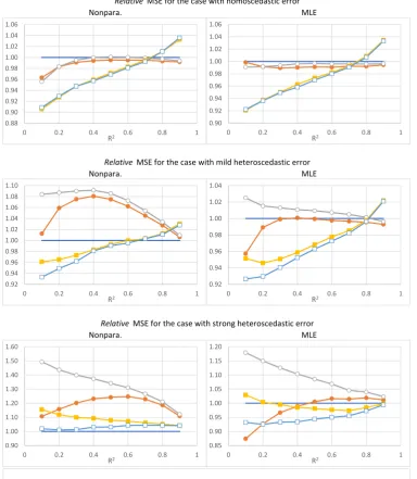
, where ˆµ₍_k₎andµ₍_k₎ are the realized vector of the estimated value ˆµand true valueµin thekthreplication, respectively. The simulation results are shown in Tables1–3. Figure1presents the same information relative to the MSE of the GLSMA method.

The results in Tables1and2show that our combination methods, MMA-GLSMA and HRCp-GLSMA, performed better than the alternatives (HRCp-GLSMA, HRCp and MMA) when the error term was homoscedastic or had mild heteroscedasticity forR2≤0.7. WhenR2≥0.8, the performance of our methods was slightly worse than that of the alternative methods. For the homoscedastic case, the three alternative methods performed similarly. On the other hand, in the case of mild heteroscedasticity, GLSMA andHRCpperformed better than MMA (which was expected, as MMA was designed for homoscedastic models).

Table3demonstrates that, when the heteroscedasticity of the error term was considerably strong, our combination method HRCp-GLSMA worked much better than the others when the MLE-based estimation ofσiwas used. However, MMA-GLSMA and HRCp-GLSMA became worse than GLSMA whenσiwas estimated using the nonparametric method.

Moreover, for most cases, GLSMA with the nonparametric estimator ofσioutperformed GLSMA with the MLE-based estimator ofσi. This can be explained by a characteristic of thek-NN method that we adopted. In thek-NN estimation, a large weight was placed on theithsquared residual to estimate σ_i2; therefore, even thoughσ_i2was misspecified, the estimate could catch the heteroscedasticity of the error term to some extent.

(7)

Relative MSE for the case with strong heteroscedastic error

Nonpara. MLE

Relative MSE for the case with mild heteroscedastic error

Nonpara. MLE

Relative MSE for the case with homoscedastic error

0.88 0.90 0.92 0.94 0.96 0.98 1.00 1.02 1.04 1.06

0 0.2 0.4 0.6 0.8 1

R2

0.90 0.92 0.94 0.96 0.98 1.00 1.02 1.04 1.06

0 0.2 0.4 0.6 0.8 1

R2

0.92 0.94 0.96 0.98 1.00 1.02 1.04 1.06 1.08 1.10

0 0.2 0.4 0.6 0.8 1

R2

0.92 0.94 0.96 0.98 1.00 1.02 1.04

0 0.2 0.4 0.6 0.8 1

R2

0.90 1.00 1.10 1.20 1.30 1.40 1.50 1.60

0 0.2 0.4 0.6 0.8 1

R2

0.85 0.90 0.95 1.00 1.05 1.10 1.15 1.20

0 0.2 0.4 0.6 0.8 1

R2

0.90 1.90

0 0.5 1

GLSMA HRCp MMA MMA‐GLSMA HRCp‐GLSMA

(8)

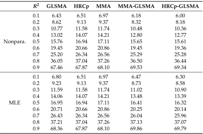
Table 1.Sample mean squared error (MSE) for the case with homoscedastic error.

R2 _GLSMA _HRCp _MMA _MMA-GLSMA _HRCp-GLSMA

0.1 6.80 6.55 6.50 6.16 6.18

0.2 9.50 9.34 9.34 8.81 8.83

0.3 12.20 12.09 12.14 11.56 11.56

0.4 15.25 15.16 15.25 14.63 14.60

Nonpara. 0.5 19.06 18.97 19.08 18.52 18.47

0.6 24.33 24.21 24.34 23.92 23.87

0.7 32.64 32.48 32.61 32.48 32.39

0.8 48.66 48.33 48.51 49.18 49.19

0.9 95.66 94.88 95.07 98.76 99.08

0.1 6.56 6.55 6.50 6.04 6.05

0.2 9.42 9.34 9.34 8.83 8.82

0.3 12.22 12.09 12.14 11.61 11.60

0.4 15.31 15.16 15.25 14.74 14.67

MLE 0.5 19.14 18.97 19.08 18.63 18.56

0.6 24.44 24.21 24.34 24.00 23.95

0.7 32.74 32.48 32.61 32.50 32.43

0.8 48.72 48.33 48.51 49.13 49.04

0.9 95.42 94.88 95.07 98.70 98.56

Table 2.Sample MSE for the case with mild heteroscedastic error.

R2 GLSMA HRCp MMA MMA-GLSMA HRCp-GLSMA

0.1 6.43 6.51 6.97 6.18 6.00

0.2 8.62 9.13 9.37 8.32 8.18

0.3 10.77 11.58 11.74 10.48 10.36

0.4 13.02 14.07 14.21 12.80 12.77

Nonpara. 0.5 15.76 16.94 17.11 15.65 15.61

0.6 19.45 20.66 20.86 19.45 19.36

0.7 25.20 26.34 26.56 25.29 25.28

0.8 36.05 37.04 37.26 36.50 36.44

0.9 67.46 67.87 68.10 69.53 69.34

0.1 6.80 6.51 6.97 6.47 6.30

0.2 9.23 9.13 9.37 8.73 8.58

0.3 11.59 11.58 11.74 11.02 10.90

0.4 14.06 14.07 14.21 13.48 13.39

MLE 0.5 16.95 16.94 17.11 16.41 16.32

0.6 20.71 20.66 20.86 20.25 20.14

0.7 26.43 26.34 26.56 26.04 25.96

0.8 37.21 37.04 37.26 37.13 37.07

0.9 68.36 67.87 68.10 69.86 69.79

Table4and5give the averages of the estimated weights corresponding to the OLS and GLS

parts for HRCp-GLSMA and MMA-GLSMA. Table 4 shows that for HRCp-GLSMA, when the

(9)

Table 3.Sample MSE for the case with strong heteroscedastic error.

R2 _GLSMA _HRCp _MMA _MMA-GLSMA _HRCp-GLSMA

0.1 13.44 14.88 20.07 15.52 13.70

0.2 16.13 18.68 23.17 18.05 16.30

0.3 18.92 22.74 26.47 20.80 19.17

0.4 22.02 27.11 30.24 24.06 22.69

Nonpara. 0.5 25.91 32.18 34.74 27.96 26.73

0.6 30.89 38.52 40.48 33.13 32.21

0.7 38.28 47.03 48.46 40.62 39.94

0.8 51.15 60.68 61.92 53.80 53.37

0.9 85.65 94.97 96.06 89.21 89.15

0.1 17.02 14.88 20.07 17.52 15.86

0.2 20.15 18.68 23.17 20.23 18.64

0.3 23.52 22.74 26.47 23.40 21.94

0.4 27.40 27.11 30.24 26.99 25.59

MLE 0.5 32.01 32.18 34.74 31.40 30.21

0.6 37.90 38.52 40.48 37.02 36.00

0.7 46.35 47.03 48.46 45.13 44.29

0.8 59.56 60.68 61.92 58.65 57.93

0.9 93.86 94.97 96.06 93.65 93.33

Table 4.Averages of the OLS ( ¯W1) and GLS ( ¯W2) parts of the weight vector for HRCp-GLSMA.

R2 0.1 0.2 0.3 0.4 0.5 0.6 0.7 0.8 0.9

Homoscedastic Cases

Nonp.OLS ( ¯W1) 0.50 0.50 0.50 0.50 0.49 0.49 0.49 0.49 0.49 Nonp. GLS ( ¯W2) 0.50 0.50 0.50 0.50 0.51 0.51 0.51 0.51 0.51 MLE OLS ( ¯W1) 0.50 0.50 0.50 0.50 0.50 0.50 0.50 0.50 0.50 MLE GLS ( ¯W2) 0.50 0.50 0.50 0.50 0.50 0.50 0.50 0.50 0.50

Mild Heteroscedastic Cases

Nonp. OLS ( ¯W1) 0.49 0.49 0.49 0.49 0.49 0.49 0.49 0.49 0.49 Nonp. GLS ( ¯W2) 0.51 0.51 0.51 0.51 0.51 0.51 0.51 0.51 0.51 MLE OLS ( ¯W1) 0.49 0.49 0.49 0.49 0.49 0.49 0.50 0.50 0.50 MLE GLS ( ¯W2) 0.51 0.51 0.51 0.51 0.51 0.51 0.50 0.50 0.50

Strong Heteroscedastic Cases

Table 5.Averages of the OLS ( ¯W1) and GLS ( ¯W2) parts of the weight vector for MMA-GLSMA.

R2 _0.1 _0.2 _0.3 _0.4 _0.5 _0.6 _0.7 _0.8 _0.9

Homoscedastic Cases

Mild Heteroscedastic Cases

Strong Heteroscedastic Cases

(10)

5. Conclusions

In this paper, we proposed a combination method of OLS and GLS estimators. The proposed method reduced the risk of misspecification between homoscedastic and heteroscedastic models. The optimality of the criteria for choosing a weight vector was proven under some regularity conditions. We performed simulation experiments to investigate the finite sample property of our combination method. The results of the simulations demonstrate that our method was adaptive for homoscedasticity and heteroscedasticity. As mentioned previously, the proposed method was novel in that it combined estimators from two different estimation methods. Combining the different estimation methods can also combine the advantages of each. This idea could be useful and should be extended to the combination of other estimation methods.

Author Contributions:This is a collaborative project. The authors are listed in alphabetical order. The proofs are done by Q. Liu.

Funding:Q. Liu acknowledges financial support from the JSPS Grant-in-Aid for Young Scientists (B) No. 25780148 and JSPS KAKENHI Grant (C) No. JP16K03590 and No. JP19K01582.

Conflicts of Interest:The authors declare no conflicts of interest.

Appendix A

For the convenience of the readers of this journal, we list Assumptions 1–3, 6 and 10–14 and replicate Lemma 7 ofLiu et al.(2016) here. Their notation ofRIn(W)coincides with our notationR(W); xmi denotes theith observation vector of the regressors of themthmodel, and xm,j,i is thejth entry ofxmi.

Assumption 1. E(|ei|4(N+1))≤c<∞for some c.

Assumption 2. ξn≡inf_W∈Hn(N)RIn(W)→∞as n→∞. Assumption 3. 0<infiσ_i2≤sup_iσ_i2<∞.

Assumption 6. The maximum eigenvalue of∑n

i=1xmix0mi/n is bounded uniformly in n and m. There exists a c>0such that the minimum eigenvalue of∑n

i=1xmix0mi/n is greater than c for any n and m. Assume thatσ_i2is a function of a finite subset ofxi, denoted byzi, so thatσ_i2=σ2(zi).

Assumption 10. σ2(·)is differentiable. Let σ0(·)denote its first derivative. Then, sup_zkσ0(z)k < ∞. Moreover, the support of ziis bounded, and the density of ziis bounded from below.

Letκbe the tuning parameter for thek-NN estimator. Letci, 1≤i≤ nbe such thatci >0 for 1≤i≤κ,ci =0 fori>κand∑κ_i₌₁ci =1.

Assumption 11. limn→∞max1≤i≤κκci<∞.

Assumption 12. limn→∞∑in=1x4m,j,i/n is bounded uniformly in m and j.

Assumption 13. There exists a C<∞such thatlimn→_∞∑n_i₌₁µ4_i/n<C.

Assumption 14. Defineν=4(N+1)and:

An = n

2/ν

√ κ

+√kl κ

+ kl

q

∑n

j=1blj2 √

κ

+κ 1/q

n1/q.

As n_√ → ∞, kl → ∞andκ → ∞, it is the case that kMAn → 0, k_M2 An/ξn → 0, nkMA2n/ξn → 0and nkMAn/ξn→0.

Lemma 7 ofLiu et al.(2016). Suppose that Assumptions 1, 3, 5, 6 and 11 of Liu, Okui and Yoshimura (2016) hold. Then, as n→∞, kl →∞andκ→∞, with k2_l/κ→0and k2_l ∑n_j₌₁b2_lj/κ→0, we have:

max i |σˇ

2

i −σ˜i2|=Op 

 kl √ κ



1+ v u u t n

∑

j=1 b2_lj



 

(11)

Proof of Lemma 1. We have:

R(W) =Ekµ−µˆ(W)k2

=E

s1µ−s1µˆols(W ∗

1) +s2µ−s2µˆgls(W2∗) 2

=Ehs21kµ−µˆols(W1∗)k2 i

(A1)

+Eh2s1s2(µ−µˆols(W1∗)) 0

µ−µˆgls(W2∗) i

(A2)

+E

s2₂

µ−µˆgls(W ∗ 2) 2 . (A3)

According toLiu and Okui(2013);Liu et al.(2016), it is obvious that the squared terms (1) and (2) are unbiased estimates of the terms (A1) and (A3) plus a constant.

In order to estimate the cross-product term (A2), we can observe that:

Y−µˆgls(W2∗)

= (µ−µˆols(W1∗)) 0

µ−µˆgls(W2∗)

+e0e +he,(I−P(W₁∗))µi+he,(I−G(W₂∗))µi −e0P(W₁∗)e−e0G(W₂∗)e

andE

e, I−P W₁∗

µ = Ehe,(I−G(W∗2))µi = 0. Therefore, the sum of the terms (3) and (4) unbiasedly estimates the cross-product term (A2).

Proof of Theorem 1. We define Lols(W) ≡ (µ−µˆols(W))

0

(µ−µˆols(W)) and Lf gls(W) ≡

µ−µˆf gls(W) 0

µ−µˆf gls(W)

. Note that:

e

CnF(W)−LF(W) =s21 h

CFMMA(W1∗)−Lols(W1∗) i

+s22 h

CIFn(W ∗

2)−Lf gls(W2∗) i

+2s1s2 n

he,(I−P(W₁∗))µi+

D

e,I−GF(W₂∗)µ E

+σˆ2tr(P(W₁∗)) +tr

GF(W₂∗)Ωˆ−e0P(W₁∗)e−e0GF(W₂∗)e

+e0e−eˆ0eˆo,

where CF_MMA = CMMA W1∗

=

2

+ 2 ˆσ2tr P W₁∗ and CF_I_n(W₂∗) =

Y−µˆgls(W ∗ 2) 2

+2tr GF(W₂∗)Ωˆ .

Using the results ofHansen(2007);Liu et al.(2016), it can be shown that the supremum with respect toW ∈ H_M(N)of all the absolute values of the terms excepte0e−eˆ0eˆdivided by risk function R(W)go to zero in probability. We only need to show:

sup W

e0e−eˆ0eˆ R(W)

→p0.

This can easily be done by modifying Lemma 7 ofLiu et al.(2016). By replacingsij, the weight defined fork-NN inLiu et al.(2016) with one, we have:

sup W

e0e−eˆ0eˆ R(W) ≤ e 0

e−e˜0e˜

/ξn+ (kL/(n−kL))e˜ 0 ˜ e/ξn

=Op 

k_l+k_l v u u t n

∑

j=1 b2 lj 

(12)

→0.

The proof is complete.

References

Danilov, Dmitry, and Jan R. Magnus. 2004. On The Harm That Ignoring Pretesting Can Cause. Journal of Econometrics122: 27–46. [CrossRef]

Hansen, Bruce E. 2007. Least Squares Model Averaging.Econometrica75: 1175–89. [CrossRef]

Hansen, Bruce E., and Jeffrey S. Racine. 2012. Jackknife Model Averaging. Journal of Econometrics167: 38–46. [CrossRef]

Li, Ker-Chau. 1987. Asymptotic Optimality forCp,CL, Cross-Validation and Generalized Cross-Validation:

Discrete Index Set.Annals of Statistics15: 958–75. [CrossRef]

Liu, Qingfeng, and Ryo Okui. 2013. Heteroscedasticity-Robust CpModel Averaging. Econometrics Journal16:

463–72. [CrossRef]

Liu, Qingfeng, Ryo Okui, and Arihiro Yoshimura. 2016. Generalized Least Squares Model Averaging.Econometric Reviews35: 1692–752. [CrossRef]

Makridakis, Spyros, Evangelos Spiliotis, and Vassilios Assimakopoulos. 2018. The M4 Competition: Results, Findings, Conclusion and Way Forward.International Journal of Forecasting34: 802–8. [CrossRef]

Wan, Alan TK, Xinyu Zhang, and Guohua Zou. 2010. Least Squares Model Averaging by Mallows Criterion.

Journal of Econometrics156: 277–83. [CrossRef]

Xie, Tian. 2017. Heteroscedasticity-Robust Model Screening: A Useful Toolkit for Model Averaging in Big Data Analytics.Economics Letters151: 119–22. [CrossRef]

Yuan, Zheng, and Yuhong Yang. 2005. Combining Linear Regression Models: When and How? Journal of the American Statistical Association100: 1202–14. [CrossRef]

Zhang, Xinyu, Alan TK Wan, and Guohua Zou. 2013. Model Averaging by Jackknife Criterion in Models with Dependent Data.Journal of Econometrics174: 82–94. [CrossRef]

Zhang, Xinyu, Guohua Zou, and Raymond J. Carroll. 2015. Model Averaging Based on Kullback-Leibler Distance.

Statistica Sinica25: 1583–98. [CrossRef] [PubMed]

Zhao, Shangwei, Aman Ullah, and Xinyu Zhang. 2018. A Class of Model Averaging Estimators.Economics Letters

162: 101–6. [CrossRef]

c