Atmos. Meas. Tech., 6, 2267–2276, 2013 www.atmos-meas-tech.net/6/2267/2013/ doi:10.5194/amt-6-2267-2013
© Author(s) 2013. CC Attribution 3.0 License.
EGU Journal Logos (RGB)
Advances in
Geosciences
Open Access
Natural Hazards
and Earth System
Sciences
Open AccessAnnales
Geophysicae
Open AccessNonlinear Processes
in Geophysics
Open AccessAtmospheric
Chemistry
and Physics
Open AccessAtmospheric
Chemistry
and Physics
Open Access DiscussionsAtmospheric
Measurement
Techniques
Open AccessAtmospheric
Measurement
Techniques
Open Access DiscussionsBiogeosciences
Open Access Open Access
Biogeosciences
Discussions
Climate
of the Past
Open Access Open Access
Climate
of the Past
Discussions
Earth System
Dynamics
Open Access Open Access
Earth System
Dynamics
DiscussionsGeoscientific
Instrumentation
Methods and
Data Systems
Open Access
Geoscientific
Instrumentation
Methods and
Data Systems
Open Access DiscussionsGeoscientific
Model Development
Open Access Open Access
Geoscientific
Model Development
DiscussionsHydrology and
Earth System
Sciences
Open AccessHydrology and
Earth System
Sciences
Open Access DiscussionsOcean Science
Open Access Open Access
Ocean Science
DiscussionsSolid Earth
Open Access Open Access
Solid Earth
DiscussionsThe Cryosphere
Open Access Open Access
The Cryosphere
DiscussionsNatural Hazards
and Earth System
Sciences
Open Access
Discussions
Dimensionality reduction in Bayesian estimation algorithms
G. W. Petty
Department of Atmospheric and Oceanic Sciences, University of Wisconsin-Madison, Madison, Wisconsin 53706, USA Correspondence to: G. W. Petty ([email protected])
Received: 15 February 2013 – Published in Atmos. Meas. Tech. Discuss.: 4 March 2013 Revised: 13 June 2013 – Accepted: 15 July 2013 – Published: 4 September 2013
Abstract. An idealized synthetic database loosely resem-bling 3-channel passive microwave observations of precipi-tation against a variable background is employed to examine the performance of a conventional Bayesian retrieval algo-rithm. For this dataset, algorithm performance is found to be poor owing to an irreconcilable conflict between the need to find matches in the dependent database versus the need to ex-clude inappropriate matches. It is argued that the likelihood of such conflicts increases sharply with the dimensionality of the observation space of real satellite sensors, which may utilize 9 to 13 channels to retrieve precipitation, for example. An objective method is described for distilling the rele-vant information content fromN real channels into a much smaller number (M) of pseudochannels while also regulariz-ing the background (geophysical plus instrument) noise com-ponent. The pseudochannels are linear combinations of the originalN channels obtained via a two-stage principal com-ponent analysis of the dependent dataset. Bayesian retrievals based on a single pseudochannel applied to the independent dataset yield striking improvements in overall performance.
The differences between the conventional Bayesian re-trieval and reduced-dimensional Bayesian rere-trieval suggest that a major potential problem with conventional multichan-nel retrievals – whether Bayesian or not – lies in the common but often inappropriate assumption of diagonal error covari-ance. The dimensional reduction technique described herein avoids this problem by, in effect, recasting the retrieval prob-lem in a coordinate system in which the desired covariance is lower-dimensional, diagonal, and unit magnitude.
1 Introduction
Satellite remote sensing entails the indirect determination of a property, or set of properties, of the environment based on measurements of top-of-the-atmosphere radiances at appro-priate wavelengths. Conceptual frameworks for undertaking satellite retrievals range from simple ad hoc methods to the iterative inversion of complex physical models of observed radiances.
For remote sensing problems involving highly non-linear and/or difficult-to-model relationships between observation vectors and environmental states, it is increasingly common to rely on so-called Bayesian estimation methods. One of the principal areas of application of Bayesian methods (but by no means the only one) has been in the area of precipitation retrieval from passive and/or active microwave observations (Evans et al., 1995; Olson et al., 1996; Haddad et al., 1997; Marzano et al., 1999; Bauer et al., 2001; Kummerow et al., 2001; Tassa et al., 2003; Di Michele et al., 2005; Grecu and Olson, 2006; Olson et al., 2006; Chiu and Petty, 2006; Viltard et al., 2006; Seo et al., 2008; Kummerow et al., 2011)
This paper has two purposes: (a) to draw attention to cer-tain practical limitations of Bayesian algorithms as typically implemented, and (b) to describe and demonstrate an objec-tive method of dimensional reduction that substantially im-proves the robustness of Bayesian retrievals in certain remote sensing applications.
The Bayesian methodology is examined here in the con-text of idealized retrievals of surface precipitation rate. How-ever, the issues raised, and their proposed solution, should have considerably broader applicability.
1.1 Bayesian estimation
Bayes’ theorem (Bayes and Price, 1763). In the present con-text, Bayes’ theorem states that the posterior probability dis-tribution function (PDF) of a desired variableRconditioned on an observation vector x is given by
P (R|x)∝P (x|R)P (R), (1)
whereP (R)is the unconditional (prior) probability density function (PDF) of the scalar variableR to be estimated and P (x|R)is the multidimensional PDF of the observation vec-tor x conditioned on a specific value ofR.
With only one known exception (Chiu and Petty, 2006), the prior joint and marginal PDFs are represented not as the continuous functions implied by Eq. (1) but rather via a large database of candidate solutions with associated ob-served or modeled multichannel radiances. This variation has been aptly called a Bayesian Monte Carlo method (L’Ecuyer and Stephens, 2002), although that more precise terminology does not seem to have achieved wider usage.
Moreover, while a true Bayes’ theorem-based retrieval should in principle be able to yield a complete posterior PDF ofR as demonstrated by Chiu and Petty (2006), it is typical in practice to extract only an expectation value based on a weighted average of the small set of discrete solution vectors in the database that approximately match the observations. For the conceptual basis and practical implementation of sev-eral Bayesian cloud and/or precipitation retrieval schemes, the reader is referred to Evans et al. (1995), Kummerow et al. (1996), Marzano et al. (1999) and L’Ecuyer and Stephens (2002).
1.2 Practical limitations
Bayes’ theorem has the advantage of providing a rigorous and complete statistical basis for optimal satellite retrievals, provided only that the requisite PDFs are known. However, this advantage can only be fully realized under fairly restric-tive conditions:
– The prior joint distribution of environmental variables must be well characterized over the full spectrum of possibilities and with adequate sampling density rel-ative to the assumed observation error (L’Ecuyer and Stephens, 2002).
– The database must be small enough to be efficiently searchable, a requirement that stands in conflict with the previous one.
– The sensor observations attached to each candidate state must be physically realistic not only on a channel-by-channel basis but also in terms of its consistency with the high-dimensional manifold encompassing actual ob-servations. This consistency can be difficult to achieve when physical model calculations, rather than actual ob-servations, supply the radiance vector (Panegrossi et al., 1998).
– The observation/modeling error covariance must be cor-rectly specified in order to optimize both the selection and the weighting of candidate solutions (L’Ecuyer and Stephens, 2002).
This paper is motivated by the observation that all of the above challenges increase exponentially as the dimensional-ity of the search space increases. For example, imagine that a mere 104solution vectors evenly distributed throughout a three-dimensional observation space is minimally adequate to characterize the prior distribution of environment states and their associated observation vectors. Depending on in-terchannel and intervariable correlations, up to 1012 candi-date solutions might be required to achieve comparable den-sity when Bayesian retrievals are directly based on the radi-ance observations of, say, a nine-channel instrument like the Tropical Rainfall Measuring Mission (TRMM) Microwave Imager (TMI; Kummerow et al., 1998).
Even if the overall density seems adequate, infrequent combinations of environmental variables – e.g., those asso-ciated with a severe storm or hurricane – will still tend to appear as outliers in an inadequately populated corner of channel space, in which case either no suitable match may be found at all or else the match sample may be small and potentially nonrepresentative.
Moreover, it usually proves difficult to confidently specify the optimal match or weighting criteria in a high-dimensional space. Formally, one usually specifies an error covariance that serves as the basis for assessing consistency between an observation vector x and a candidate solution in the database. In practice, the full covariance is rarely known and only an assumed per-channel error variance is usually specified. This is the approach taken by the current version of the Goddard Profiling (GPROF) algorithm for TRMM (Kummerow et al., 2011), for example, among many other retrieval and assimi-lation schemes.
Note further that while the formal error covariance follows from an analysis of model and/or instrument error alone, this specification is only useful if the database is densely popu-lated relative to that expected error. When the density is low, as is especially the case for less common scenes, one must often either arbitrarily expand the the search neighborhood until one or more nominal matches are found or else flag the retrieval for that observation as “missing” owing to a failure to find matches within the prescribed tolerance.
some conditions, especially when the correct solutions lie in close proximity to incorrect solutions. As will be demon-strated below, the inappropriate assumption of diagonal co-variance can severely degrade retrieval performance. 1.3 Objectives
In this paper, we demonstrate some important practical limi-tations of the Bayesian method as typically applied to satel-lite retrievals. Rather than use real satelsatel-lite data, we construct an idealized synthetic database comprising only three simu-lated “channels” and associated with a single scene variable, “rain rate”. These channels are subject to considerable vari-ability due to prescribed background noise. As is character-istic of passive microwave observations of precipitation over land, the signal due to rain rate is intentionally weak in ab-solute magnitude relative to the background noise but with a spectral component that is distinct from the background vari-ability.
We first show that conventional Bayesian retrievals in 3-channel space can lead to nearly useless estimates owing to match failures and/or over-averaging. We then demonstrate a technique for reducing the dimensionality of the database and for obtaining significantly more robust retrievals from the same data and using the same Bayesian framework. In effect, we derive a smaller number of “pseudochannels” – i.e., linear transformations of the original channels or sim-ple functions thereof – that retain most of the desired signal while rejecting a large part of the background noise. What remains of the background noise is decorrelated and scaled to unit variance.
Note that while the benefits of appropriate dimensional re-duction should hold in general for any database-type retrieval problem, the particular dimensional reduction algorithm de-scribed below is most directly applicable to semi-continuous variables like rain rate or cloud liquid water path for which admissible values are either exactly zero or positive.
2 Synthetic database
A Gaussian pseudorandom number generator was used to create 20 000 vectors of 3-channel “background brightness temperatures” with prescribed mean x=(220,240,250)and covariance
S=
506 81−205 81 173 140 −205 140 269
. (2)
These statistical properties are arbitrary apart from the desire that the synthetic data lie on an oblique 3-D plane with added uncorrelated random noise having unit variance.
For 10 % of these scenes, a non-zero rain rateR was as-signed. This rain rate obeys a half-Gaussian (positive only) distribution with unit standard deviation. The unique spec-tral signature of the rain is described by a unit vector aˆ=
(0.366,−0.682,0.633), so that raining scenes are simply non-raining scenes with an added brightness temperature perturbation given by Ra. This idealized rain signal is ofˆ course considerably cleaner than that encountered in real satellite observations and serves our purpose of highlighting retrieval issues associated strictly with the Bayesian frame-work as opposed to the physics.
This dataset is split evenly into a “training dataset” (TRAIN) and a “validation dataset” (VAL), each consist-ing of 10 000 “observations”. Our objective is to utilize the TRAIN data to implement a Bayesian algorithm capable of achieving reasonable performance when applied to the inde-pendent VAL data. Because the two datasets are statistically identical, problems we identify will be associated exclusively with issues relating to sampling density and dimensionality, not to representativeness or modeling error.
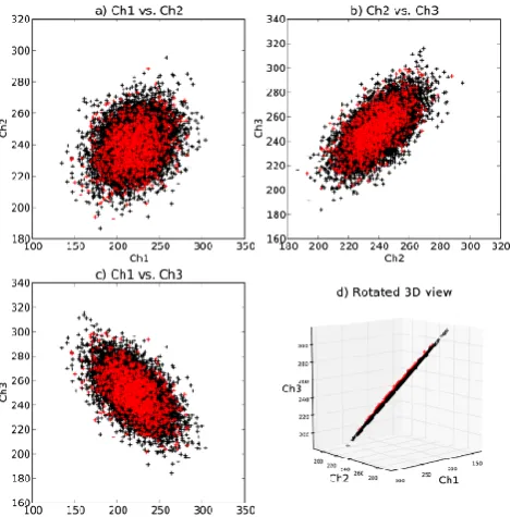
Two-dimensional scatter plots for each possible pair of channels are depicted for the TRAIN data in Fig. 1a–c. It is clear from these plots that no pair of raw channels is suf-ficient to distinguish “raining” and “non-raining” scenes. It is not even evident from the 2-D depictions that any useful radiometric distinction exists.
In fact, the background noise in this demonstration is con-fined to a three-dimensional plane (apart from 1 K Gaussian noise), and the subtler rain “signature”a has, by design, aˆ small component normal to that plane (Fig. 1d). It is this very subtle separation, which only even exists in a 3-D framework, which we must exploit if we wish to retrieve rainfall against the very noisy background. This case also illustrates the dan-ger in relying on 1-D or 2-D projects of multidimensional observation vectors to assess the retrievability of a particular variable.
The question addressed in the next section is whether a conventional Bayesian retrieval algorithm that relies on “brute force” matching of observations in 3-channel space and employing the usual assumption of diagonal error co-variance can successfully pull the relatively weak rain signal out of the much larger-magnitude background noise.
3 Bayesian retrieval in channel space
3.1 Method
We begin with a straightforward retrieval method concep-tually similar to that currently used for TMI and envis-aged as well for the future Global Precipitation Measure-ment Microwave Imager (GMI). The TRAIN data serves as a database that is searched for scenes that match a given observation vector to within a specified tolerance. Specifi-cally, each prospective match is assigned a weight given by w=exp(−s), where
s=X i
xi−x0 i σi
2
Fig. 1. Scatter plots of an idealized, stochastically generated database consisting of 3-channel brightness temperatures. Black markers are used for non-raining scenes; red markers indicate rain-ing scenes. (a) Channel 1 vs. channel 2. (b) Channel 2 vs. channel 3. (c) Channel 1 vs. channel 3. (d) A rotated 3-D plot revealing that the non-raining scenes lie primarily in a 3-channel plane, with raining pixels exhibiting slight separation.
wherexiis the observation from theith channel,xi0is the cor-responding value for the database entry, andσi is a channel-dependent uncertainty that captures modeling error and/or observation error. As previously noted, a rigorous calcula-tion ofsshould actually be based on a full error covariance matrix S, of whichσi2are the diagonal elements, but this is typically not done. For the idealized experiments described herein, we takeσ to have the same value for all channels.
Consistent with the current implementation of the God-dard Profiling algorithm (Kummerow et al., 2001, 2011) for the TMI, we admit only matches for whichw >0.01. The retrieval for a given observation vector is then given by
ˆ R=
PP j=1wjRj0 PP
j=1wj
, (4)
whereP is the number of qualifying matches.
For a given observation vector x, we require at leastN=1 to have any valid retrieval at all; largerN will improve the statistical representativeness of the retrieval and may permit error statistics to be derived as well. In principle, we can al-ways increaseσ until sufficient matches are found, but the benefits of increased sample size must be weighed against the loss of retrieval quality that results from treating increas-ingly dissimilar scenes as “matches”.
As noted earlier, the problem of finding matches within a sufficiently small neighborhood of the observation is de-pendent on the local density of the training sample in obser-vation space. The higher-dimensional the obserobser-vation space, the larger the training database must be to ensure adequate density in any given neighborhood. Moreover, extreme val-ues of the variable to be retrieved will usually occupy the most sparsely populated regions in channel space.
3.2 Application to TRAIN data
It is instructive to apply the above algorithm to the same ob-servations stored in the TRAIN database, not only as a san-ity check but to illustrate an important consideration in the choice ofσ. We know that even an arbitrarily small value of σ will still yield an exact match in every case, because each observation passed to the algorithm is present in the database. Of interest here is what happens when the tolerance is loos-ened so as to find additional matches.
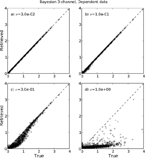
Figure 2 depicts scatter plots of the retrieved versus ac-tual rain rate for four different choices of σ. Forσ=0.03 (Fig. 2a), the agreement is essentially perfect, because for each observation, exactly one match is found, and that match is the observation itself. But forσ >0.1 (Fig. 2b–d), there is an increasing tendency toward underestimation of the true rain rate, because now dissimilar scenes are being included in the average, most of which have a significantly differ-ent (usually zero) rain rate. Forσ=1.0 (Fig. 2d), the result is nearly useless on a pixel-by-pixel basis, even though the mean rain rate for all pixels will still be correct.
The initial conclusion to draw from this comparison is that even when exact matches to all observations are available in the database, the use of an inappropriately large value forσ will seriously degrade the retrievals.
3.3 Application to VAL data
We now apply the same algorithm to the independent VAL data. Statistically, these data are identical to those in the TRAIN database, but there are likely to be very few exact matches. Consequently, when σ=0.03, the match failure rate is an unacceptably large 94 % (Fig. 3a). Moreover, the failure rate is highest by far for the non-zero rain rate scenes, since these are more thinly spread in channel space.
Fig. 2. Results of a Bayesian retrieval algorithm applied to the 3-channel dependent (TRAIN) dataset for four different values of the error parameterσ.
algorithm performance, despite our reliance on a database of 10 000 entries populating a mere three-dimensional observa-tion space.
The GPROF algorithm, to give one example, recognizes this problem and undertakes multiple passes through the database. If a match is not found for a given value ofσ, the value is doubled and the search repeated. In this way, it is ensured that matches will eventually be found for all obser-vations, albeit with very loose tolerances for the rarest com-binations of channel values.
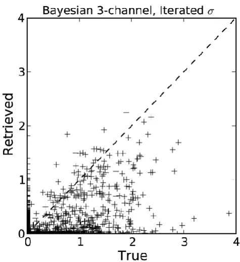
Figure 4 illustrates the results of this procedure applied to our synthetic database. There are now no match failures, but the quality of the retrieval remains poor, with a great many underestimated values of larger rain rates and a similar num-ber of non-zero retrievals where there the true value is zero. Less apparent is that this procedure does not even conserve the ensemble averaged rain rate for the entire dataset – the av-erage for all 10 000 points is only 39 % of the true value. This is because non-raining scenes typically find matches for low values ofσ so that only other non-raining (or low-raining) scenes are included in the retrieval, while high rain rates in the tail of the distribution typically require largeσ with the consequent incorporation of poorer matches (typically lower rain rates) into the retrieval.
Fig. 3. Same as Fig. 2, but the Bayesian algorithm is applied to the independent (VAL) dataset. Also indicated is the percentage of observations for which no match could be found for the given value ofσ.
3.4 Preliminary assessment
In view of the poor performance of the Bayesian scheme in the above demonstration, one might reasonably ask whether the signal-to-noise ratio is simply too poor in the synthetic dataset for any retrieval method to yield high-quality results, at least using a solution database comprising only 10 000 en-tries.
In fact, it will be shown shortly that retrieval performance is markedly improved simply by first applying an operator that retains sensitivity to the rain rate signal while rejecting most of the background noise, and by using the single result-ing pseudochannel as an index into the TRAIN database.
4 Dimensional reduction
4.1 General goals
In the present context, the process of dimensional reduction entails the following:
Fig. 4. Results of the Bayesian algorithm applied to the independent (VAL) dataset, using iterative doubling ofσ to ensure that matches are found for all observations.
2. From those first-stage transformed channels, perform a second linear transformation that collects most of the sensitivity to the desired variable (e.g., rain or cloud) into a significantly smaller number of pseudochannels. 3. Utilize those pseudochannels in place of the larger
number of original channels in a lower-dimensional Bayesian retrieval scheme.
Note that while principal component analysis (PCA) is uti-lized in the first two steps and is, in general, a common method for dimensional reduction, a single-stage PCA de-composition of a dataset does not accomplish either of the two steps on its own. In particular, ordinary PCA provides no direct basis for distinguishing between the desired signa-ture and the undesirable noise. Indeed, in our example, the desired signature is conventionally associated with the least important principal component as measured by its contribu-tion to the total variance, and would normally be discarded in the most common approach to dimensional reduction using PCA.
4.2 Details
4.2.1 Stage 1
The following procedure is applied to pixels for which the variabley to be retrieved is zero. In the present case, this condition is satisfied by 90 % of the database, or 9000 obser-vations.
First, we compute the meanhXiand the covariance Sxfor the rain-free pixels. From Sx, we then compute the eigenvec-tors Exand eigenvalues3x. We define the first-stage trans-formed channels y via
yi =λ−1/2x,i [(x− hxi)TEx]i. (5) That is, we take the projection of(x− hxi)onto theith eigen-vector and then scale by square root of the eigenvalue to ob-tain unit variance. With appropriate definitions of the coeffi-cient matrix A, the above operation reduces to
y=A(x− hxi). (6)
hyi =0 and Sy=I for the set of transformed channels when observing the background only, but they otherwise retain all of the same information as found in the original x, Thus, we may now conveniently treat the total background noise (in-strument plus geophysical) as having unit variance and zero correlation between transformed channels y.
Figure 5a depicts the results of the transformation applied to the synthetic data. The background noise (black markers) has been sphered and has unit variance.
4.2.2 Stage 2
The first stage PCA alone provides no guidance as to which components in the transformed space are associated with the desired signal. We therefore now also apply Eq. (6) to the 10 000 precipitating scenes yr withR >0 (red markers in Fig. 5). Unlike the case for rain-free scenes, there is no con-straint on the variance of the raining scenes, and it is expected that any existing separation in the original dataset will be amplified in absolute terms. To objectively isolate the added variance due to rain, we compute Sy,r≡ hyryrTi and com-pute eigenvectors Ey,rand eigenvalues3y,r.
We now define the precipitation pseudochannels
z≡yTEy,r. (7)
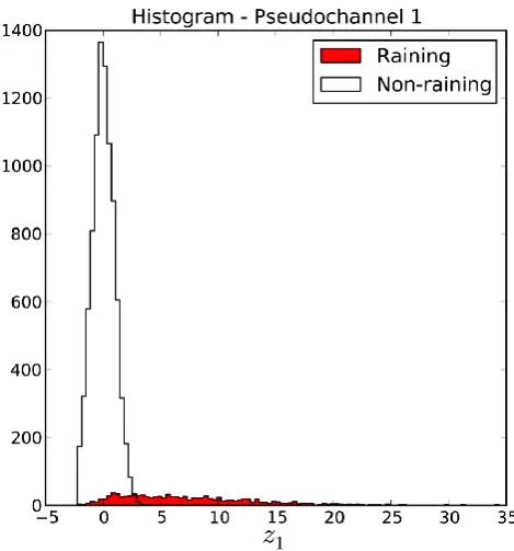
Outside of precipitation, these pseudochannels still have zero mean and unit uncorrelated variance. For precipitating scenes, however, the added variability will have been pushed into the first few eigenvectors Ey,r. In Figs. 5 and 6, we see that the first pseudochannelz1now captures all of the useable spectral distinction between “rain” and “no rain”.
In the more general case, we might keep the firstM ele-ments of z so as to account for at least, say, 95 % of the vari-ance computed from the sums of the eigenvalues. The rest are discarded. For the synthetic dataset discussed above,M=1. In the paper by Petty and Li (2013), which begins with the 9 channels of the TMI,M=3.
The first- and second-stage linear transformation may be combined to give
Fig. 5. Results of the two-stage transformation applied to the raw channel data depicted in Fig. 1. (a) The first-stage transformation, from Eq. (5). (b) The second-stage transformation, from Eq. (7).
where B is anM×N array of coefficients consistent with Eqs. (5) and (7). Note, by the way, that for the present dataset, B is a vector corresponding in direction to the third eigen-vector of the complete dataset. We could have arrived at B more directly in this particular case, but the dimensional re-duction algorithm described above works well for a higher-dimensional dataset, unlike the case for conventional single-stage PCA, which, as noted earlier, provides no basis for as-signing eigenvectors to specific geophysical signatures.
Fig. 6. Histograms of the first pseudochannelz1for non-raining and raining scenes.
5 Bayesian retrieval in pseudochannel space
Using the pseudochannel transformations derived above, we may undertake Bayesian retrievals inM-dimensional space rather than the originalN-dimensional space. The procedure is otherwise identical to that described in Sect. 3. For our synthetic database,M=1.
Figure 7 depicts results of the algorithm applied to the de-pendent (TRAIN) data for selected values of σ, analogous to Fig. 2 (note that values ofσ here cannot be directly com-pared with the values ofσ for the 3-D retrievals, owing to the difference in scaling of the observation vector). We see an increase in retrieval error with larger values ofσ, but the degradation is not nearly as severe as was the case for the original retrieval using three channels.
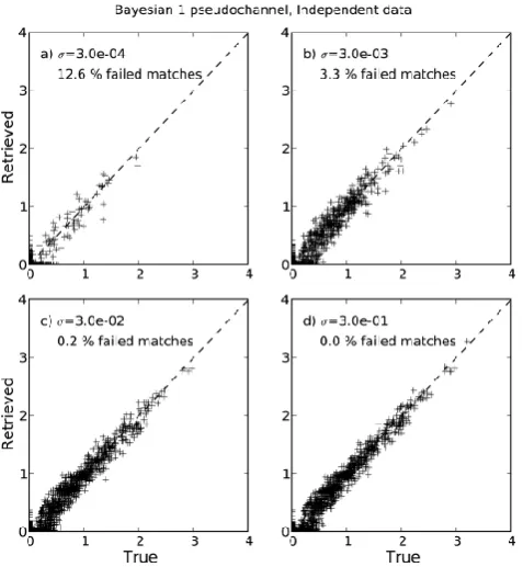
Figure 8 depicts results for the independent (VAL) data, analogous to Fig. 3. The improvement relative to 3-D re-trieval is striking. The match failure rate is extremely low for all but the smallest values ofσ, and the errors are gen-erally small and unbiased. For larger values ofσ, there is a hint of underestimation at the low end of the scale owing to inclusion of nearby zero values.
Fig. 7. Similar to Fig. 2, but the Bayesian retrieval applied to the dependent (TRAIN) dataset is based on a one-dimensional pseu-dochannel rather than the original three-dimensional brightness temperatures.
Fig. 8. Same as Fig. 7, but the Bayesian 1-D retrieval is applied to the independent (VAL) data.
Fig. 9. Results of the 1-D Bayesian algorithm applied to the inde-pendent (VAL) dataset, using iterative doubling ofσto ensure that matches are found for all observations. Compare with the 3-D re-trievals depicted in Fig. 4.
6 Conclusions and discussion
Starting with an idealized synthetic database that loosely re-sembles 3-channel passive microwave observations of pre-cipitation against a highly variable background (e.g., het-erogeneous land surfaces and/or land–water mixes), we ex-amined the performance of a conventional Bayesian re-trieval algorithm that searched for matches in the full three-dimensional channel space. First we showed that even when the algorithm is applied to the dependent (TRAIN) data, per-formance suffers when the match criterion is too loose (i.e., largeσ). Conversely, when the same algorithm was applied to the independent (VAL) dataset, the match failure rate was unacceptably high unless the match criterion was loose.
The net result of both effects was that retrievals were quite poor for the independent dataset, even whenσwas iteratively adjusted, as shown in Fig. 4. Of course, the need to use large σ to overcome a high match failure rate is a function of the size of the dependent dataset. In the present demonstration, the TRAIN dataset consisted of 10 000 unique entries. If we were to employ a much larger database, the match failure rate would go down, allowing smallerσ and presumably leading to improved overall performance.
the database required to adequately populate the observa-tion space and thus to ensure not only the existence of suit-able matches for any given observation but also, it would be hoped, a statistically representative distribution of such matches.
Of course it might be possible to reduce dimensionality in some cases by simply throwing out channels that are deemed to provide little information. As clearly seen in Fig. 1, this would not have been possible in the present demonstration. With higher-dimensional real satellite data, the decision as to which channels do or do not contain useful information is nontrivial and undoubtedly context dependent.
To mitigate the problem of dimensionality in Bayesian re-trievals, we described an algorithm for objectively distill-ing the relevant information content from N channels into a smaller number (M) of pseudochannels while also regu-larizing the background (geophysical plus instrument) noise component. In the present demonstration,N=3 andM=1. In the application of this method to TMI data described by Petty and Li (2013),N=9 andM=3.
Bayesian retrievals based on the single pseudochannel de-rived for the synthetic dataset were shown to yield striking improvements in overall performance, as shown in Fig. 9. These empirical results, more than any theoretical arguments, underline the likely benefits of dimensional reduction in Bayesian retrievals relying on a database of multichannel ob-servations as a proxy for the prior joint and marginal PDFs.
It must be reiterated that the details of the particular di-mensional reduction method given here depend on one being able to stratify the dependent dataset into two subsets: one representing the “pure” background (e.g., rain-free or cloud-free), and the other representing non-zero values of the vari-able to be retrieved (e.g., raining or cloudy). For varivari-ables where this is not possible, another dimensional reduction al-gorithm would need to be employed; however, the benefits for Bayesian retrievals should be similar.
As discussed in the introduction, it might have been pos-sible in principle to achieve the same results for the 3-D channel-based retrieval as for the 1-3-D pseudochannel-based retrieval, provided that an appropriate covariance ma-trix were specified for the computation of the weights for candidate matches. In the present demonstration, the covari-ance in question would have corresponded to a match zone shaped like a highly flattened spheroid oriented exactly par-allel to the plane containing most of the background vari-ability in Fig. 1. That is, channel variations orthogonal to the principal plane of background variability would be given far greater weight than variations spectrally consistent with the background variability. In short, the appropriate covariance would be non-diagonal, and retrieval performance would de-pend strongly on getting it exactly right.
From our results and from the above considerations, we conjecture that a major potential problem with conven-tional multichannel retrievals and assimilation schemes – whether Bayesian or not – lies in the very common but often
inappropriate assumption of diagonal error covariance. The dimensional reduction technique described herein avoids this problem by, in effect, recasting the retrieval problem in a co-ordinate system in which the desired covariance is (a) lower-dimensional, (b) diagonal, and (c) unit magnitude.
Acknowledgements. Helpful comments by Tristan L’Ecuyer,
Filipe Aires, and an anonymous reviewer led to significant im-provements in the manuscript. This research was supported by NASA Grant NNX10AGAH69G.
Edited by: F. S. Marzano
References
Bauer, P., Amayenc, P., Kummerow, C., and Smith, E.: Over-ocean rainfall retrieval from multisensor data of the Tropical Rainfall Measuring Mission. Part II: Algorithm implementation, J. At-mos. Ocean Tech., 18, 1838–1855, 2001.
Bayes, T. and Price, R.: An Essay towards Solving a Problem in the Doctrine of Chances. By the Late Rev. Mr. Bayes, F. R. S. communicated by Mr. Price, in a Letter to John Canton, A. M. F. R. S., Philosophical Transactions, 53, 370–418, 1763.
Bellman, R.: Adaptive Control Processes: A Guided Tour, Princeton University Press, 1961.
Chiu, J.-Y. and Petty, G.: Bayesian retrieval of complete posterior PDFs of oceanic rain rate from microwave observations, J. Appl. Meteorol. Clim., 45, 1073–1095, 2006.
Di Michele, S., Tassa, A., Mugnai, A., Marzano, F., Bauer, P., and Baptista, J.: Bayesian algorithm for microwave-based precipita-tion retrieval: Descripprecipita-tion and applicaprecipita-tion to TMI measurements over ocean, IEEE T. Geosci. Remote, 43, 778–791, 2005. Evans, K., Turk, J., Wong, J., and Stephens, T.: A Bayesian
ap-proach to microwave precipitation profile retrieval, J. Appl. Me-teorol., 34, 260–279, 1995.
Grecu, M. and Olson, W.: Bayesian estimation of precipitation from satellite passive microwave observations using combined radar-radiometer retrievals, J. Appl. Meteorol. Clim., 45, 416–433, 2006.
Haddad, Z., Smith, E., Kummerow, C., Iguchi, T., Farrar, M., Durden, S., Alves, M., and Olson, W.: The TRMM “day-1” radar/radiometer combined rain-profiling algorithm, J. Meteorol. Soc. Jpn., 75, 799–809, 1997.
Kummerow, C., Olson, W., and Giglio, L.: A simplified scheme for obtaining precipitation and vertical hydrometeor profiles from passive microwave sensors, IEEE T. Geosci. Remote, 34, 1213– 1232, 1996.
Kummerow, C., Barnes, W., Kozu, T., Shiue, J., and Simpson, J.: The Tropical Rainfall Measuring Mission (TRMM) sensor pack-age, J. Atmos. Ocean Tech., 15, 809–817, 1998.
Kummerow, C., Hong, Y., Olson, W., Yang, S., Adler, R., McCol-lum, J., Ferraro, R., Petty, G., Shin, D., and Wilheit, T.: The evo-lution of the Goddard profiling algorithm (GPROF) for rainfall estimation from passive microwave sensors, J. Appl. Meteorol., 40, 1801–1820, 2001.
Mi-crowave Rainfall Retrievals, J. Atmos. Ocean Technol., 28, 113– 130, 2011.
L’Ecuyer, T. and Stephens, G.: An uncertainty model for Bayesian Monte Carlo retrieval algorithms: Application to the TRMM observing system, Q. J. Roy. Meteorol. Soc., 128, 1713–1737, 2002.
Marzano, F., Mugnai, A., Panegrossi, G., Pierdicca, N., Smith, E., and Turk, J.: Bayesian estimation of precipitating cloud parame-ters from combined measurements of spaceborne microwave ra-diometer and radar, IEEE T. Geosci. Remote, 37, 596–613, 1999. Olson, W., Kummerow, C., Heymsfield, G., and Giglio, L.: A method for combined passive-active microwave retrievals of cloud and precipitation profiles, J. Appl. Meteorol., 35, 1763– 1789, 1996.
Olson, W., Kummerow, C., Yang, S., Petty, G., Tao, W., Bell, T., Braun, S., Wang, Y., Lang, S., Johnson, D., and Chiu, C.: Pre-cipitation and latent heating distributions from satellite passive microwave radiometry. Part I: Improved method and uncertain-ties, J. Appl. Meteorol. Clim., 45, 702–720, 2006.
Panegrossi, G., Dietrich, S., Marzano, F., Mugnai, A., Smith, E., Xiang, X., Tripoli, G., Wang, P., and Baptista, J.: Use of cloud model microphysics for passive microwave-based precipitation retrieval: Significance of consistency between model and mea-surement manifolds, J. Atmos. Sci., 55, 1644–1673, 1998.
Petty, G. and Li, K.: Improved passive microwave precipitation re-trievals over land and ocean. 1. Algorithm description., J. At-mos. Ocean. Technol., online first, doi:10.1175/JTECH-D-12-00144.1, 2013.
Seo, E.-K., Sohn, B.-J., Liu, G., Ryu, G.-H., and Han, H.-J.: Im-provement of microwave rainfall retrievals in Bayesian retrieval algorithms, J. Meteorol. Soc. Jpn., 86, 405–409, 2008.
Tassa, A., Di Michele, S., Mugnai, A., Marzano, F. S., and Poiares Baptista, J. P. V.: Cloud model–based Bayesian tech-nique for precipitation profile retrieval from the Tropical Rainfall Measuring Mission Microwave Imager, Radio Science, 38, 8074, doi:10.1029/2002RS002674, 2003.