Atmos. Meas. Tech., 6, 3359–3368, 2013 www.atmos-meas-tech.net/6/3359/2013/ doi:10.5194/amt-6-3359-2013
© Author(s) 2013. CC Attribution 3.0 License.
Atmospheric
Measurement
Techniques
Open Access
Cloud discrimination in probability density functions of
limb-scattered sunlight measurements
E. N. Normand1, J. T. Wiensz2, A. E. Bourassa1, and D. A. Degenstein1 1Institute of Space and Atmospheric Studies, University of Saskatchewan, Canada 2SRON Netherlands Institute for Space Research, Utrecht, Netherlands
Correspondence to: A. E. Bourassa ([email protected])
Received: 19 April 2013 – Published in Atmos. Meas. Tech. Discuss.: 16 July 2013 Revised: 31 October 2013 – Accepted: 4 November 2013 – Published: 9 December 2013
Abstract. A technique characterizing the distribution of
cir-rus cloud-top occurrences from the Optical Spectrograph and Infrared Imaging System (OSIRIS) limb-scattering radiance profiles is presented. The technique involves computing scat-tering residual profiles by comparing normalized measured radiance and modelled molecular radiance profiles where en-hancements in the measured radiance indicate the presence of clouds. Probability density functions of scattering residuals show the distribution is not a continuum measurement; there is a distinction between the cloudy and cloud-free conditions. Observations show high cloud-top occurrences in the upper troposphere and lower stratosphere region above Indonesia and Central America. Results obtained using this technique with OSIRIS measurements are compared to those obtained by Sassen et al. (2008) with Cloud-Aerosol Lidar Pathfinder Satellite Observations (CALIPSO) nadir measurements and to those obtained by Wang et al. (1996) with Stratospheric Aerosol and Gas Experiment (SAGE) II solar occultation measurements.
1 Introduction
Clouds have pivotal influence on the Earth’s hydrological cycle and climate system because they are intricately in-volved in the dynamical, chemical, and radiative processes within the upper troposphere and lower stratosphere (UTLS) (Chahine, 1992; Liou, 1992; Hobbs, 1993). Cirrus clouds oc-cur at high altitude around the tropopause level and, despite their thin appearance and low optical thickness, they have an important contribution to the radiative balance of the at-mosphere (Liou, 1986, 2002). The processes in this region
of the atmosphere have become increasingly important for a clear understanding of feedback mechanisms in the climate system.
Detecting and discriminating clouds can be non-trivial. Cloud visibility depends on several factors such as the viewing geometry of the measuring instrument; the relative brightness between the targeted cloud and its background; and the scattering phase function, which characterizes scat-tering directionality (Sassen et al., 1989). The optical thick-ness,τ, which is a function of wavelength, is a critical com-ponent affecting visibility. Sassen and Cho (1992) catego-rized cirrus clouds into three groups according to their optical thickness: subvisual clouds withτ <0.03, threshold visible withτ ≈0.03, and thin cirrus withτ >0.03. Optically thin clouds are below the detection threshold of passive nadir-viewing instruments, yet they scatter light sufficiently to bias their trace gas retrievals. By contrast, in limb-scattering or occultation geometries, even very optically thin clouds can produce a measurable effect on the measured brightness pro-file.
3360 E. N. Normand et al.: Cloud discrimination in probability density functions
Absorption SpectroMeter for Atmospheric CHartographY) measurements were used by Eichmann et al. (2010) in a multi-wavelength approach to determine global cloud-top heights, and von Savigny et al. (2004) developed a technique for detection of noctilucent clouds. Limb-emission measure-ments in the infrared have also been employed for studying clouds. Greenhough et al. (2005) used MIPAS (Michelson Interferometer for Passive Atmospheric Sounding) measure-ments to retrieve a cloud detection index, and Sembhi et al. (2012) studied MIPAS detection limits for cloud and aerosol particles. We use measurements from the Optical Spectro-graph and Infrared Imaging System (OSIRIS), a Canadian satellite instrument that measures atmospheric limb profiles of scattered solar radiation, along with a statistical approach to characterize and discriminate cloud scattering.
A detailed description of the cloud detection technique is presented and the results obtained using the technique are compared to those by Sassen et al. (2008), who used Cloud-Aerosol Lidar Pathfinder Satellite Observations (CALIPSO) nadir measurements and to those by Wang et al. (1996), who used Stratospheric Aerosol and Gas Experiment (SAGE) II solar occultation measurements of cirrus clouds.
2 Measurements and modelling
OSIRIS (Llewellyn et al., 2004), a Canadian instrument on-board the Swedish Odin satellite (Murtagh et al., 2002), was designed to measure vertical profiles of atmospheric limb ra-diance of scattered sunlight from the upper troposphere to the lower mesosphere.
Odin was launched 20 February 2001 into a sun-synchronous orbit with a period of 96 min. The orbital in-clination of 98◦from the Equator provides near-global cov-erage as the corresponding sampled latitude range for nomi-nal on-track instrument pointing is from 82◦S to 82◦N. The satellite track is near-terminator, implying a dawn–dusk or-bit. The entire atmosphere at the tangent point is illuminated when the solar zenith angle is less than 90◦. As such, the win-ter hemisphere is largely in darkness at the local time. Over the course of a year, both the solar zenith angle and the solar scattering angle vary between 60◦and 120◦(Murtagh et al., 2002).
OSIRIS is composed of two optical modules: the optical spectrograph (OS), which is of main interest in this work, and the infrared imager. The OS consists of an optical grating and a CCD detector and measures atmospheric limb radiance be-tween 280 and 810 nm with a spectral resolution of approx-imately 1 nm. The OS has a single line of sight, and vertical profiles from roughly 7 to 110 km in altitude are obtained by nodding the entire spacecraft; this facilitates obtaining ob-servations over a range of tangent altitudes (Murtagh et al., 2002). The OS has a 1 km vertical and approximately 40 km horizontal field of view at the tangent point. Successive mea-surements are separated by roughly 2 km tangent altitude. It
takes nearly 1.5 min to complete a full vertical scan; thus there are about 60 scans per orbit. Refer to Llewellyn et al. (2004) for a complete description of the instrument.
SASKTRAN (Bourassa et al., 2008) is a spherical ge-ometry radiative transfer model designed to simulate limb-scattered solar radiation. It solves the equation of radia-tive transfer through the method of successive orders for rays travelling within the spherical geometry in order to ac-curately and efficiently account for the multiple-scattering contribution to the limb radiance. The method of succes-sive orders is used to obtain a solution describing light that has undergone multiple scattering by computing scat-tering solutions recursively. When modelling the scatscat-tering of light by aerosols, SASKTRAN accounts for an altitude-dependent cross section and phase function. Absorption by numerous temperature-dependent species is also considered in the model. SASKTRAN is used for operational retrievals of ozone, nitrogen dioxide, and aerosols from the OSIRIS measurements. In this work, SASKTRAN is used to model the radiance from the molecular background in an aerosol-and cloud-free atmosphere within a limb geometry. The air number density is taken from European Centre for Medium-Range Weather Forecasts (ECMWF) reanalysis interpolated in time and space to the position of the OSIRIS measurement.
2.1 Single scattering in an optically thin atmosphere
The radiative transfer equation considering only a single-scattering event of a solar photon in the atmosphere,I1, is
I1(r0,)ˆ = ˜I1(s1,)eˆ −τ (s1,0)+ 0 Z
s1
κ(s)J1(s,)eˆ −τ (s,0)ds, (1)
whereI˜1is the radiance from the end of the line of sight;r0 is the satellite position; ands1 is the position of the single-scattering event alongs, the axis running along the line of sight. The single-scattering source term,J1(s,)ˆ , is
J1(s,)ˆ =
κscat(s)
κ(s) F0( ˆ
0)e−τ (sun,s)P (s,,ˆ ˆ0), (2)
whereκscat(s)is the scattering extinction,F0(ˆ0)is the so-lar irradiance,τ (sun, s)is the optical depth from the Sun to the scattering point, and P (s,,ˆ ˆ0)is the effective phase function for scattering from the solar direction,ˆ0, into the propagation direction,ˆ, and has units per steradian.
In Eq. (1), the exponentiale−τ (s1,0) in the first term
E. N. Normand et al.: Cloud discrimination in probability density functions 3361
sight that ends in deep space. Successive rays in the multiple-scatter calculation that strike the ground include this term as ground scatter.
This integral is largely dominated by the tangent point con-tribution, so for an optically thin atmosphere – that is, when
τ1 – the radiance is
I1(r0,)ˆ ≈κ(sT)J1(sT,)1sˆ T,
≈κscat(sT)F0(ˆ0)P (s,,ˆ ˆ0)1sT, (3) where1sTis the tangent point path length andP (s,,ˆ ˆ0) is the scattering phase function which describes the proba-bility of scattering in a direction. When a number of particles and molecules contribute to the scattering of light, the radi-ance is a sum over each scattering contributor. In the case of an atmosphere containing background molecular nitrogen and oxygen as well as particles such as aerosols and clouds, the radiance for an optically thin atmosphere, which is pro-portional to the number density of the scattering contributors, is
I1(r0,)ˆ ≈
h
nscatm(sT)σscatm(sT)Pm(s,,ˆ ˆ0)
+nscatp(sT)σscatp(sT)Pp(s,,ˆ ˆ0) i
F0(ˆ0)1sT, (4) where the subscripts m and p denote molecular background and particle scattering, respectively.
3 Cloud detection technique
3.1 Scattering residual and probability density functions
In the limb geometry, the Earth’s atmosphere is optically thin down to upper tropospheric tangent altitudes for wavelengths longer than around 700 nm. For this analysis, OSIRIS mea-surements at 800 nm were used; this is essentially the longest wavelength measured by OSIRIS that is not contaminated by polarization anomalies caused by the grating. As seen in Eq. (4), the measured radiance,Imeasured, can be split into two components: that due to the molecular background,Imolecular, and due to clouds and aerosols,Iparticles.
The SASKTRAN model was used to approximate the molecular background radiance within an atmosphere free of aerosols and clouds. By comparing of the measured radi-ance profiles from OSIRIS to the modelled ones obtained us-ing SASKTRAN, the radiance contribution from clouds and aerosols can be quantified.
The measured radiance and modelled molecular radiance profiles were directly compared after employing a tangent al-titude normalization. The reference tangent alal-titude was cho-sen nearest 35 km because it is typically cloud- and aerosol-free at this altitude and because OSIRIS measurements above this altitude start to become contaminated by larger noise due to exponentially falling signal levels. Only scans taken
during the descending track of Odin’s orbit were considered, which, for a short time period and narrow latitude band, the scattering angle is roughly constant.
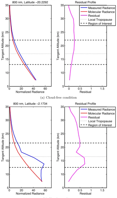
In a cloud- and aerosol-free atmosphere, the normalized measured radiance,I˜measured, and the normalized molecular radiance, I˜modelled, profiles should essentially agree within the accuracy of the optically thin approximation. The limb radiance is approximately exponential in altitude for an op-tically thin atmosphere. The discrepancy between the curves within 12 and 35 km tangent altitudes, shown in the left plot of Fig. 1a, is enhanced scattering due to stratospheric aerosol. Further discrepancies in the measurements indicate the pres-ence of additional aerosol or cloud scattering. We define the difference between the logarithm of the measured and mod-elled molecular radiance as a scattering residual,R, that can be used to characterize scattering enhancements,
R=ln
˜ Imeasured
˜ Imodelled
!
. (5)
In a cloud-free atmosphere, the residual values in the right-hand plot of Fig. 1a hover around zero except in the re-gion where there is a contribution from stratospheric aerosol. Figure 1b shows a positive enhancement between 13.7 and 16.1 km tangent altitudes, suggesting the presence of clouds. Scattering residual profiles were generated and used to create histograms of scattering residuals. In the absence of clouds the residual values linger around zero, so collectively they form a histogram peak near zero and represent the cloud-free condition. In the event of a cloud, scattering is enhanced so the residual values are much greater and form a second histogram peak. The histogram was normalized by the total number of measurements to obtain a probability density function (PDF). The tangent altitude regions of in-terest, which are defined by the local tropopause of the scan, were defined to be 1 km thick and a residual PDF was made for each region. The local tropopause height is defined by the cold point tropopause and is calculated from ECMWF re-analysis at OSIRIS scan points. For a given latitudinal band, these PDFs form a two-dimensional probability density sur-face shown in Fig. 2. The left maximum range represents the cloud-free condition and the smaller right maximum range represents the cloudy condition. An interesting and useful property of these PDFs is that the distribution in the resid-ual PDF is not a continuum measurement. The separation of the peaks, which is a significant result, provides a clear indi-cation of the ability to distinguish the two conditions.
3.2 Cloud-free threshold as a function of altitude
3362 E. N. Normand et al.: Cloud discrimination in probability density functions
latitudinal band, the PDF is integrated from the threshold po-sition over the cloudy condition.
Figure 2 shows the cloud-free threshold curve as a function of altitude overtop the probability density surface for scans in the Northern Hemisphere tropical latitudinal band in Au-gust 2007 at 800 nm. The distributions corresponding to the cloud-free and cloudy conditions gradually shift to slightly higher residual values as altitude increases due to increasing stratospheric aerosol concentration with altitude. Thus, the threshold distinguishing the two conditions is a curved line as a function of altitude. Although they maintain the same general shape, the maxima cloud-free and cloudy distribu-tions are also different for each latitudinal band due to shift-ing satellite viewshift-ing geometry and any atmospheric variation with latitude. Therefore, each two-dimensional probability density surface requires a unique cloud-free threshold curve. A technique was developed to determine the threshold based on the PDFs.
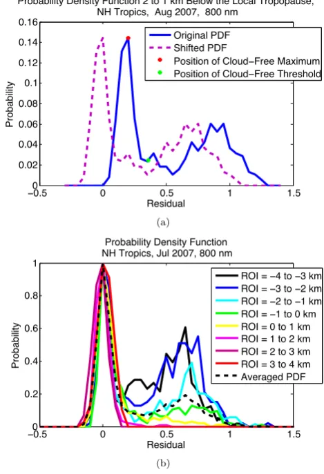
For each altitude region of interest, the maximum of the cloud-free peak was found and the distance from zero along the residual axis,δi, was noted, whereidenotes theith
alti-tude region of interest (ROI). The PDF was then normalized by the maximum value of the cloud-free peak and shifted as to align the maximum with zero. This process is shown in Fig. 3a. Once the PDFs from each altitude region were shifted, the PDFs were normalized and averaged to obtain the averaged PDF, which is shown in Fig. 3b.
The average cloud-free distribution can be closely approx-imated by a Gaussian distribution. However, the presence of some residual scattering on the positive side of the peak causes a skew in the distribution. Therefore, the left-hand side of the averaged cloud-free maximum peak was mir-rored to obtain a Gaussian-type mirmir-rored shape. The mirmir-rored shape was then fit to a Gaussian.
The variance of the fitted Gaussian, σ2, was computed such that
σ=|√xo−µ|
2 ln 2, (6)
wherexoandµare the half-width, half-maximum position
and the mean of the fitted Gaussian, respectively. The posi-tion 2σwas found to be a reliable demarkation of the thresh-old position between the cloud-free and cloudy conditions. As latitude increases, the distinction between the cloud-free and cloudy distributions becomes blurred, especially near lower tangent altitudes. To determine the cloud-free thresh-old curve as a function of altitude, the 2σ position to the right of the cloud-free peak maximum was determined on the PDFs for each altitude region of interest. That is, the PDFs from each altitude region of interest from Fig. 3 were un-shifted by δi, the distance the original PDF was shifted to
zero along the residual axis, and the position 2σ to the right of the maximum of the cloud-free peak was marked as the threshold point.
Discussion
P
ap
er
|
Dis
cussion
P
ap
er
|
Discussion
P
ap
e
r
|
Discussion
P
ap
er
|
0 20 40 60
5 10 15 20 25 30 35
Normalized Radiance
Tangent Altitude (km)
800 nm, Latitude −20.2292
0 0.5 1 1.5
5 10 15 20 25 30 35
Residual
Tangent Altitude (km)
Residual Profile
Measured Radiance Molecular Radiance Residual Local Tropopause Region of Interest
Student Version of MATLAB
(a) Cloud-free condition
0 20 40 60
5 10 15 20 25 30 35
Normalized Radiance
Tangent Altitude (km)
800 nm, Latitude −2.1734
0 0.5 1 1.5
5 10 15 20 25 30 35
Residual
Tangent Altitude (km)
Residual Profile
Measured Radiance Molecular Radiance Residual Local Tropopause Region of Interest
Student Version of MATLAB
(b) Cloudy condition
Figure 1: Normalized radiance, density, and residual profiles as a function of
tangent altitude at 800 nm for(a)cloud-free and(b)cloudy conditions. These
profiles were measured in May 2007.
1
Fig. 1.
Normalized radiance, density, and residual profiles as a function of tangent altitude at 800 nm for
(a)
cloud-free and
(b)
cloudy conditions. These profiles were measured in May 2007.
21
Fig. 1. Normalized radiance, density, and residual profiles as a func-tion of tangent altitude at 800 nm for (a) cloud-free and (b) cloudy conditions. These profiles were measured in May 2007.
The validity of the cloud-free threshold curve is illustrated by computing the residuals,R, from simulated OSIRIS mea-surements through cirrus clouds. This radiative transfer mod-elling of simulated OSIRIS measurements was done with SASKTRAN by assuming cloud-scattering properties from the in situ database of Baum et al. (2005). The cloud particle number density profile,n(h), is assumed to be Gaussian and is scaled to give a prescribed value of cloud optical thickness,
τc. The vertical extent of the cloud is defined as the full width at half-maximum (FWHM) of the distribution. Both the use of a single effective particle size and horizontal homogene-ity within the cloud layer are assumed. For more details on model configurations, see Wiensz et al. (2013).
E. N. Normand et al.: Cloud discrimination in probability density functions 3363
2D Probability Density Function NH Tropics, Aug 2007, 800 nm
Tangent Altitude wrt Local Tropopause (km)
Residual
0 0.5 1 1.5
−4 −3 −2 −1 0 1 2 3
P
ro
b
a
b
ilit
y
0 0.05 0.1 0.15 0.2 0.25 0.3 Cloud−Free
Threshold
Cloud−
Free Cloudy
c=0.03
Fig. 2. Two-dimensional residual probability density function (PDF) with the cloud-free threshold curve (dashed green) and cor-responding modelled subvisual cirrus curve for cirrus optical thick-nessτc=0.03 (solid magenta) for scans within the Northern Hemi-sphere tropical latitudinal band in August 2007 at 800 nm. The ver-tical axis is shown with respect to the local tropopause.
descending-node OSIRIS scan at a latitude of 7◦N.
Simulated tangent altitudes were fixed with respect to the lo-cal tropopause altitude. To study the perturbation to the val-ues ofRfrom a cirrus cloud at varying altitudes, successive model runs were done with a given cloud (with fixed vertical and optical thickness) as it moved upward through the tan-gent altitudes. The cloud “bottom” in each case is made to coincide with the line-of-sight tangent altitude to ensure that each line of sight passes directly through the bulk scattering region of the cloud as it is shifted. Residuals were computed from the modelled radiances by Eq. (5). For each set of mod-elled radiances, which correspond to varying cloud altitude, the maximum residual occurs at the tangent altitude pass-ing through the bulk of the cloud. This value is taken as the residual for the cloud altitude. The curve of computed resid-ual,R, as a function of cloud altitude is shown in Fig. 2 for cirrus optical thicknessτc=0.03, which is the subvisual cir-rus detection threshold (Sassen and Cho, 1992). Simulations were done for cloud effective particle sizeDe=40 µm and vertical thickness 200 m.
The figure illustrates several key points. First, the cloud-free threshold lies at values ofR well below those for sub-visual cirrus clouds. This suggests that the threshold indeed forms a demarcation between regions that contain relatively weakly and strongly scattering particles. Second, it is no-table that the area of decreased probability between the two “branches” in the figure lies at altitudes and residuals be-tween the threshold curve and the subvisual cirrus curve. This indicates an increased occurrence of thin clouds at val-uesτc≥0.03 relative to lowerτcvalues.
Discussion
P
ap
er
|
Dis
cussion
P
ap
er
|
Discussion
P
ap
e
r
|
Discussion
P
ap
er
|
−00.5 0 0.5 1 1.5
0.02 0.04 0.06 0.08 0.1 0.12 0.14 0.16
Residual
Probability
Probability Density Function 2 to 1 km Below the Local Tropopause, NH Tropics, Aug 2007, 800 nm
Original PDF Shifted PDF
Position of Cloud−Free Maximum Position of Cloud−Free Threshold
(a)
−00.5 0 0.5 1 1.5
0.2 0.4 0.6 0.8 1
Residual
Probability
Probability Density Function NH Tropics, Jul 2007, 800 nm
ROI = −4 to −3 km ROI = −3 to −2 km ROI = −2 to −1 km ROI = −1 to 0 km ROI = 0 to 1 km ROI = 1 to 2 km ROI = 2 to 3 km ROI = 3 to 4 km Averaged PDF
(b)
Figure 3: (a)Probability density function for scans within 2 to 1 km below the tropopause within the Northern Hemisphere tropical latitudinal band in Au-gust 2007 at 800 nm. (b)Normalized and shifted probability density functions for various altitude regions of interest (ROI) and averaged probability density function for scans within the Northern Hemisphere tropical latitudinal band in July 2007 at 800 nm.
3
Fig. 3. (a)
Probability density function for scans within 2 to 1 km below the tropopause within the
North-ern Hemisphere tropical latitudinal band in August 2007 at 800 nm.
(b)
Normalized and shifted
prob-ability density functions for various altitude regions of interest (ROI) and averaged probprob-ability density
function for scans within the Northern Hemisphere tropical latitudinal band in July 2007 at 800 nm.
23
Fig. 3. (a) PDF for scans within 2 to 1 km below the tropopause within the Northern Hemisphere tropical latitudinal band in Au-gust 2007 at 800 nm. (b) Normalized and shifted PDFs for various altitude regions of interest (ROI) and averaged PDF for scans within the Northern Hemisphere tropical latitudinal band in July 2007 at 800 nm.
3.3 Change in solar scattering angle with time
3364 E. N. Normand et al.: Cloud discrimination in probability density functions
Discussion
P
ap
er
|
Dis
cussion
P
ap
er
|
Discussion
P
ap
e
r
|
Discussion
P
ap
er
|
Jul06 Oct06 Jan07 Apr07
75 80 85 90 95 100 105 110
Time
Solar Scattering Angle (degrees)
Solar Scattering Angle Over Time
Fig. 4.Solar scattering angle as a function of time from June 2006 to June 2007.
24
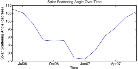
Fig. 4. Solar scattering angle as a function of time from June 2006 to June 2007.
When data spanning a large time period are used to form a single PDF, the distributions are blurred as if there were several time-dependent PDFs overlaid on top of each other. Because the amplitude of the measured signal changes over time due to changing solar scattering angles, it is necessary to separate the data into time-dependent sections as to produce PDFs with little blurring. In this work, data were separated into monthly bins where a two-dimensional PDF, such as that shown in Fig. 2, was made and a unique threshold line was computed for each latitude range and for each month consid-ered.
3.4 Cloud-top correction
The OSIRIS scans were organized on a monthly basis into bins according to their latitude and longitude coordinates, where the latitudinal and longitudinal bins were 7.5◦and 20◦
wide, respectively. A probability density surface of scattering residuals was created from radiance profiles. A cloud-free threshold curve was determined for each month and latitude band. By integrating from this line over the cloudy maximum range, the probability of locating a cloud for a given altitude range within a latitude–longitude bin on a monthly basis was determined. As neither the vertical thickness nor the horizon-tal extent of the clouds were taken into account, these prob-abilities are biased. In order to avoid a counting bias, clouds should only be detected once at the highest detected tangent altitude.
To correct this bias, each scan was checked for residual values that fell in the tangent altitude region of interest be-yond the cloud-free threshold curve. The cloud-free thresh-old curve is a function of altitude; the dashed green line in Fig. 2 separates the cloud-free and cloudy conditions. Thus, the threshold curve was overlaid on the residual profile. The first and highest cloud occurrence beyond the threshold curve was noted and all other residual values below this altitude were disregarded. Therefore, rather than simply detecting the presence of a cloud at a given altitude, the results show the detection of cloud tops; that is, the highest measurement that shows the presence of cloud.
4 Comparison to CALIPSO
In an effort to validate and test the cloud detection technique, results using OSIRIS data are compared to those obtained by Sassen et al. (2008), who utilized CALIPSO measurements.
CALIPSO is a joint satellite mission between NASA Lan-gley Research Center and CNES to investigate the impact clouds and aerosols have on the radiative balance of the at-mosphere. CALIPSO was launched April 2006 into a cir-cular sun-synchronous polar orbit at about 705 km altitude. Like Odin, CALIPSO has an orbital inclination of 98◦from the Equator which provides global coverage from 82◦S to 82◦N. The satellite retraces its track to within±10 km every 16 days (Winker et al., 2004, 2007).
Among the three nadir-viewing instruments onboard CALIPSO, Cloud-Aerosol Lidar with Orthogonal Polariza-tion (CALIOP) is a polarizaPolariza-tion-sensitive lidar and takes measurements of the total attenuated backscatter at 532 and 1064 nm. The lidar profiles contain information on the ver-tical distribution of clouds and aerosols, the ice–water phase composition of the clouds through the ratio of the signals from two orthogonal polarization channels, and the size dis-tribution of aerosol particles through the wavelength depen-dence of the backscatter signal (Winker and Pelon, 2003).
Sassen et al. (2008) studied the global distribution of cirrus clouds from CALIPSO measurements from 15 June 2006 to 15 June 2007. A cirrus cloud identification algorithm was de-veloped to assure only cirrus clouds detected by CALIPSO were used in the analysis. Additional constraints were ap-plied to the data to void detections of polar stratospheric clouds (PSCs) and ice clouds occurring at unusually low al-titudes. Lastly, in order to distinguish cloud layers, clouds must be separated by a minimum of 1.0 km in height (Sassen et al., 2008).
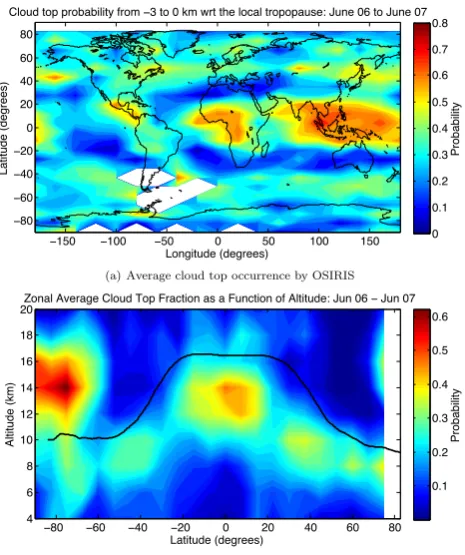
Figure 1 of Sassen et al. (2008) shows the global distri-bution of the average cirrus cloud occurrence frequency as detected by the CALIPSO identification algorithm in terms of 5.0◦ longitude and 5.0◦ latitude grid boxes. Figure 2 of Sassen et al. (2008) displays the equivalent distribution as altitude versus latitude in 0.2 km height intervals and 2.5◦ latitude bins. For comparison, the analogous average cloud-top occurrence frequency of clouds detected by OSIRIS us-ing the cloud detection technique are shown in Fig. 5a and b, respectively, with 20◦ longitude and 7.5◦ latitude grid boxes and 2 km height intervals. The comparisons reveal good agreement especially considering the different viewing geometries of the instruments.
E. N. Normand et al.: Cloud discrimination in probability density functions Discussion 3365
P
ap
er
|
Dis
cussion
P
ap
er
|
Discussion
P
ap
e
r
|
Discussion
P
ap
er
|
Longitude (degrees)
Latitude (degrees)
Cloud top probability from −3 to 0 km wrt the local tropopause: June 06 to June 07
−150 −100 −50 0 50 100 150
−80 −60 −40 −20 0 20 40 60 80
Probability
0 0.1 0.2 0.3 0.4 0.5 0.6 0.7 0.8
Student Version of MATLAB (a) Average cloud top occurrence by OSIRIS
Zonal Average Cloud Top Fraction as a Function of Altitude: Jun 06 − Jun 07
Altitude (km)
Latitude (degrees)
−80 −60 −40 −20 0 20 40 60 80
4 6 8 10 12 14 16 18 20
Probability
0.1 0.2 0.3 0.4 0.5 0.6
Student Version of MATLAB (b) Zonal average cloud top occurrence by OSIRIS
Figure 5: (a)Average cloud top occurrence frequency of clouds detected by
OSIRIS algorithm in a three-kilometer thick layer below the local tropopause
between June 2006 and June 2007. (b) Zonal average cloud top occurrence
frequency of clouds detected by OSIRIS algorithm between June 2006 and June 2007.
5
Fig. 5. (a)Average cloud top occurrence frequency of clouds detected by OSIRIS algorithm in a
three-kilometer thick layer below the local tropopause between June 2006 and June 2007.(b)Zonal average cloud top occurrence frequency of clouds detected by OSIRIS algorithm between June 2006 and June 2007.
25
Fig. 5. (a) Average cloud-top occurrence frequency of clouds de-tected by OSIRIS algorithm in a 3 km thick layer below the local tropopause between June 2006 and June 2007. (b) Zonal average cloud-top occurrence frequency of clouds detected by OSIRIS al-gorithm between June 2006 and June 2007.
south-east Asian rainforest, the rainforests in Central Amer-ica and in the Amazon region, and the Congo Basin rainforest in Africa (Wang et al., 1996; Dessler and Sherwood, 2004; Fu et al., 2007; Sassen et al., 2009). The minima bands along
±30◦latitude correspond to the dry downwelling on the edge of the Hadley cells.
From Fig. 5b, the latitudinal distribution shows maxi-mum cirrus cloud occurrence within the tropical belt between
±15◦latitude at 14 km altitude, which is coincident with the mean location of the Intertropical Convergence Zone (ITCZ) and the level of maximum convective outflow. There is also about 23 % cloud occurrence in the lower stratosphere within the tropics. These ultra-thin stratospheric clouds are observed by OSIRIS but are not detected by CALIPSO, likely due to differing instrument sensitivities and viewing geometries. Cirrus cloud occurrence generally decreases as the poles are approached except at the South Pole, where the presence of PSCs dominate. PSCs occur well within the stratosphere near 14 km at high southern latitudes and were removed from the CALIPSO detections. As latitude increases, the cloud-free and cloudy PDF distributions, as in Fig. 2, tend to merge at the lower tangent altitudes, which at these latitudes is closer to the tropopause, and increases the uncertainty in the tech-nique.
5 Comparison to SAGE II
The cloud detection technique with OSIRIS limb-scattering measurements is further compared to those obtained by Wang et al. (1996), who used SAGE II occultation measure-ments as the viewing geometries of these two instrumeasure-ments are similar.
The SAGE II instrument was aboard the Earth Radiation Budget Satellite and its mission was to measure the verti-cal profiles of ozone, nitrogen dioxide, water vapour, and the aerosol extinction coefficient. The satellite flew in a sun-synchronous orbit with a 90 min period and a 57◦ inclina-tion to allow a latitudinal coverage of approximately 135◦ per month. The latitude extremes varied seasonally; however there was no sampling poleward of 55◦ during boreal and austral winters (Wang et al., 1996).
SAGE II was a seven-channel radiometer with channels centred at 0.385, 0.448, 0.453, 0.525, 0.600, 0.940, and 1.02 µm. The instrument used the solar occultation technique capturing 15 sunrise events in one day. These were approxi-mately equally separated in longitude and exhibited a slight shift in latitude between consecutive measurements. The in-strument’s field of view was 0.5 km vertically and 2.5 km horizontally at the tangent point (Wang et al., 1996).
Wang et al. (1996) assembled a climatology of cloud oc-currence frequency based on six years of SAGE II observa-tions between 1985 and 1990. Subvisual and opaque clouds were distinguished by the measurement upper limit extinc-tion coefficient for aerosols. Using the cirrus cloud classifica-tion from Sassen and Cho (1992), clouds with extincclassifica-tion co-efficients larger than the measurement limit were marked as opaque clouds because the transmitted signal fell beyond the instrument’s sensitivity and the cloud profile was restricted to that altitude (Wang et al., 1996). Furthermore, clouds were distinguished from aerosols through the ratio of the extinc-tion coefficients at two wavelengths, namely at 0.52 and 1.02 µm. Such a ratio contains information on the particle size.
Fueglistaler et al. (2009) compared the mean cirrus cloud occurrence frequencies for opaque and cirrus clouds derived from CALIPSO and SAGE II instruments in Fig. 9a and b of Fueglistaler et al. (2009), respectively. Although both in-struments demonstrate that thinner cirrus clouds occur within the tropical tropopause layer and opaque clouds occur at lower altitudes, the curves illustrating the occurrence fre-quencies do not agree well. Theτ <0.03 thin line in Fig. 9b of Fueglistaler et al. (2009) should be contained within the
3366 E. N. Normand et al.: Cloud discrimination in probability density functionsDiscussion
P
ap
er
|
Dis
cussion
P
ap
er
|
Discussion
P
ap
e
r
|
Discussion
P
ap
er
|
0 20 40
5 10 15 20
Occurrence Frequency, %
Altitude, km
NH Middle Lat SH Middle Lat NH Tropic Lat SH Tropic Lat
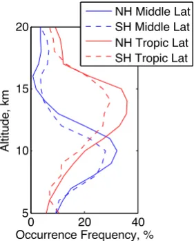
Fig. 6.Mean cloud occurrence frequency versus altitude as measured by OSIRIS from June 2006 to June 2007. Tropical and mid-latitudinal bands were defined as0≤θ <25and25≤θ <55in their respective hemispheres.
26
Fig. 6. Mean cloud occurrence frequency versus altitude as mea-sured by OSIRIS from June 2006 to June 2007. Tropical and mid-latitudinal bands were defined as 0≤θ <25 and 25≤θ <55 in their respective hemispheres.
curves agree nicely with the SAGE II thin cirrus curve. This result is encouraging especially because the two instruments have similar viewing geometries. OSIRIS detected roughly 10 % more cirrus clouds than SAGE II possibly because of a higher limb-viewing sensitivity. This result leads to a confir-mation of the theory presented in Fueglistaler et al. (2009).
Plate 1a of Wang et al. (1996) shows the global distri-bution of cirrus cloud occurrence frequency between 1985 and 1990 as measured by SAGE II. This figure can be com-pared to Fig. 1 of Sassen et al. (2008) and Fig. 5a. Note, however, that the data used in these figure do not cover the same time period, so differences are to be expected. The comparison between figures must be carried out with care as the figures using CALIPSO and SAGE II data are pro-duced on an absolute altitude scale, while the OSIRIS anal-ysis utilizes an altitude scale relative to the local tropopause. The OSIRIS analysis was carried out in this way to compen-sate how the tropopause height falls in altitude as the poles are approached. Similarly, the 6 yr average zonal mean oc-currence frequency distribution of SAGE II subvisual clouds is shown in Fig. 2a of Wang et al. (1996) and can be com-pared to Fig. 2 of Sassen et al. (2008) and Fig. 5b. In agree-ment between these figures and Fig. 6, the maximum cirrus cloud occurrence is between 14 and 15 km altitude within the tropical latitudinal band. While there are differences between CALIPSO, SAGE II, and OSIRIS measurements, the general positions and magnitudes of the maxima and minima cloud occurrence frequencies occur in relatively close agreement.
To assure adequate sampling, Wang et al. (1996) aver-age six years of SAGE II occultation data together. Since OSIRIS captures enough sampling to form yearly figures, an average figure representing multiple years of data is not necessary and an analysis can be made on a yearly basis. In
Discussion
P
ap
er
|
Dis
cussion
P
ap
er
|
Discussion
P
ap
e
r
|
Discussion
P
ap
er
|
Longitude (degrees)
Latitude (degrees)
Cloud top probability from −3 to 0 km wrt the local tropopause: June 05 to June 06
−150 −100 −50 0 50 100 150
−80
−60
−40
−20 0 20 40 60 80
Probability
0 0.1 0.2 0.3 0.4 0.5 0.6 0.7 0.8
Student Version of MATLAB (a)
Longitude (degrees)
Latitude (degrees)
Cloud top probability from −3 to 0 km wrt the local tropopause: June 07 to June 08
−150 −100 −50 0 50 100 150
−80
−60
−40
−20 0 20 40 60 80
Probability
0 0.1 0.2 0.3 0.4 0.5 0.6 0.7 0.8
Student Version of MATLAB (b)
Longitude (degrees)
Latitude (degrees)
Cloud top probability from −3 to 0 km wrt the local tropopause: June 08 to June 09
−150 −100 −50 0 50 100 150 −80
−60 −40 −20 0 20 40 60 80
Probability
0 0.1 0.2 0.3 0.4 0.5 0.6 0.7 0.8
Student Version of MATLAB (c)
Figure 7: Yearly average cloud top occurrence frequency of clouds detected by OSIRIS algorithm in a three-kilometer thick layer below the local tropopause.
7
Fig. 7.
Yearly average cloud top occurrence frequency of clouds detected by OSIRIS algorithm in a
three-kilometer thick layer below the local tropopause.
27
Fig. 7. Similar to Fig. 5a, yearly average cloud-top occurrence fre-quency of clouds detected by OSIRIS algorithm in a 3 km thick layer below the local tropopause.
E. N. Normand et al.: Cloud discrimination in probability density functions 3367
6 Conclusions
OSIRIS employs the limb-scattering technique and measures the radiance of the atmosphere to infer information on the distribution of ozone, nitrogen dioxide, and aerosols within the stratosphere. Although clouds are not measured directly, OSIRIS measurements are used in the development of a high-altitude cloud detection technique.
The efficiency and reliability of the cloud detection tech-nique depends on the residual profile’s ability to characterize the occurrence of clouds. The scattering residual is computed as the logarithmic difference between the measured radiance profile at 800 nm where the atmosphere is optically thin down to tropospheric altitudes and the modelled molecular radi-ance profile. PDFs are produced from the scattering residual profiles for separate latitudinal bands on a monthly basis. Be-cause the solar scattering angle changes over the course of a year, the variation in the amplitude of the measured radiance signal causes a shift in the PDF distribution along the residual axis. Thus, producing separate time-resolved PDFs prevents blurring distributions.
The PDFs reveal the scattering residual distribution is not a continuum measurement. The ability to distinguish the cloudy and cloud-free conditions is key to the success of the technique. A Gaussian curve is used to model the cloud-free distribution. Threshold residual lines are drawn as a function of altitude two standard deviations to the right of the cloud-free range along the residual axis and delimit the occurrence of clouds. By overlaying these threshold lines onto the resid-ual profiles, the presence of a cloud within the altitude region of interest can be determined. Comparison of the cloud-free threshold with residuals from radiative transfer simulations with known cirrus cloud conditions indicates that the method of threshold selection is reasonable.
A useful application of the cloud detection technique is to produce probability maps showing the distributions of cloud-top occurrence frequencies. Cloud-cloud-top maxima were found over Central America and over Indonesia as these correspond to highly convective regions, and minima bands were located along±30◦latitude on the edge of the Hadley cells.
Fueglistaler et al. (2009) showed profiles of the mean cloud occurrence frequency versus altitude in the tropics as measured by CALIPSO and SAGE II and theorized that the inconsistency between the profiles is a result of the differ-ent viewing geometries and optical depth thresholds of the instruments. For comparison, the cloud detection technique was used to plot the cloud-top occurrence frequency ver-sus altitude profiles derived from OSIRIS measurements for tropical and mid-latitude regions. The shape of the tropical profiles compared relatively well with the analogous cirrus cloud profile from SAGE II, which is an encouraging result because SAGE II and OSIRIS have similar viewing geome-tries.
The applications and use of the cloud detection tech-nique have not been exhausted in this work. Since complex
radiative transfer is required to accurately model scattering through optically thick layers of atmosphere or clouds, the cloud detection technique can be used to identify the pres-ence of clouds as well as the cloud-top altitude within the scans. Furthermore, the cloud detection technique can be em-ployed to study the evolution of cloud-top occurrence fre-quencies and distributions as well as to detect PSCs at high southern latitudes during austral spring.
Acknowledgements. This work was supported by the Natural Sciences and Engineering Research Council (Canada) and the Canadian Space Agency. Odin is a Swedish-led satellite project funded jointly by Sweden (SNSB), Canada (CSA), France (CNES) and Finland (Tekes).
Edited by: A. Kokhanovsky
References
Baum, B. A., Heymsfield, A. J., Yang, P., and Bedka, S. T.: Bulk Scattering properties for the remote sensing of ice clouds. Part I: Microphysical Data and Models, J. Appl. Meteor., 44, 1885– 1895, 2005.
Bourassa, A. E., Degenstein, D. A., and Llewellyn, E. J.: SASK-TRAN: a spherical geometry radiative transfer code for efficient estimation of limb scattered sunlight, J. Quant. Spectrosc. Ra., 109, 52–73, 2008.
Chahine, M. T.: The hydrological cycle and its influence on climate, Nature, 359, 373–380, doi:10.1038/359373a0, 1992.
Dessler, A. E. and Sherwood, S. C.: Effect of convection on the summertime extratropical lower stratosphere, J. Geophys. Res., 109, D23301, doi:10.1029/2004JD005209, 2004.
Eichmann, K.-U., Bovensmann, H., Meringer, M., von Savigny, C., and Kokhanovsky, A.: 38th COSPAR Scientific Assembly, 38, p. 104, 2010.
Fu, Q., Hu, Y., and Yang, Q.: Identifying the top of the tropical tropopause layer from vertical mass flux analysis and CALIPSO lidar cloud observations, Geophys. Res. Lett., 34, L14813, doi:10.1029/2007GL030099, 2007.
Fueglistaler, S., Dessler, A. E., Dunkerton, T. J., Folkins, I., Fu, Q., and Mote, P. W.: Tropical tropopause layer, Rev. Geophys., 47, RG1004, doi:10.1029/2008RG000267, 2009.
Greenhough, J., Remedios, J. J., Sembhi, H., and Kramer, L. J.: Towards cloud detection and cloud frequency distributions from MIPAS infra-red observations, Adv. Space Res., 36, 800–806, doi:10.1016/j.asr.2005.04.096, 2005.
Hobbs, P. V.: Aerosol-Cloud-Climate Interactions, Academic Press, San Diego, Ca., USA, 1993.
Liou, K. N.: Influence of cirrus clouds on weather and climate processes: a global perspective, Mon. Weather Rev., 114, 1167, doi:10.1175/1520-0493(1986)114<1167:IOCCOW>2.0.CO;2, 1986.
Liou, K. N.: Radiation and Cloud Processes in the Atmosphere, Ox-ford Univ. Press, New York, N. Y., USA, 1992.
3368 E. N. Normand et al.: Cloud discrimination in probability density functions
Llewellyn, E. J., Lloyd, N. D., Degenstein, D. A., Gattinger, R. L., Petelina, S. V., Bourassa, A. E., Wiensz, J. T., Ivanov, E. V., McDade, I. C., Solheim, I. C., McConnell, J. C., Haley, C. S., von Savigny, C., Sioris, C. E., McLinden, C. A., Griffioen, E., Kaminski, J., Evans, W. F., Puckrin, E., Strong, K., Wehrle, V., Hum, R. H., Kendall, D. J. W., Matsushita, J., Murtagh, D. P., Brohede, S., Stegman, J., Witt, G., Barnes, G., Payne, W. F., Piché, L., Smith, K., Warshaw, G., Deslauniers, D.-L., Marc-hand, P., Richardson, E. H., King, R. A., Wevers, I., Mc-Creath, W., Kyrölä, E., Oikarinen, L., Leppelmeier, G. W., Auvi-nen, H., Mégie, G., Hauchecorne, A., Lefèvre, F., de La Nöe, J., Ricaud, P., Frisk, U., Sjoberg, F., von Schéele, F., and Nordh, L.: The OSIRIS instrument on the Odin spacecraft, Can. J. Phys., 82, 411–422, doi:10.1139/P04-005, 2004.
Murtagh, D., Frisk, U., Merino, F., Ridal, M., Jonsson, A., Stegman, J., Witt, G., Eriksson, P., Jiménez, C., Megie, G., de La Noë, J., Ricaud, P., Baron, P., Pardo, J. R., Hauch-corne, A., Llewellyn, E. J., Degenstein, D. A., Gattinger, R. L., Lloyd, N. D., Evans, W. F. J., McDade, I. C., Haley, C. S., Sioris, C., von Savigny, C., Solheim, B. H., McConnell, J. C., Strong, K., Richardson, E. H., Leppelmeier, G. W., Kyrölä, E., Auvinen, H., and Oikarinen, L.: Review: An overview of the Odin atmospheric mission, Can. J. Phys., 80, 309–319, doi:10.1139/P01-157, 2002.
Sassen, K. and Cho, B. S.: Subvisual-thin cirrus lidar dataset for satellite verification and climatological research, J. Appl. Meteorol., 31, 1275–1285, doi:10.1175/1520-0450(1992)031<1275:STCLDF>2.0.CO;2, 1992.
Sassen, K., Griffin, M. K., and Dodd, G. C.: Optical scattering and microphysical properties of subvisual cirrus clouds, and climatic implications, J. Appl. Meteorol., 28, 91–98, doi:10.1175/1520-0450(1989)028<0091:OSAMPO>2.0.CO;2, 1989.
Sassen, K., Wang, Z., and Liu, D.: Global distribution of cir-rus clouds from CloudSat/Cloud-Aerosol Lidar and Infrared Pathfinder Satellite Observations (CALIPSO) measurements, J. Geophys. Res., 113, D00A12, doi:10.1029/2008JD009972, 2008.
Sassen, K., Wang, Z., and Liu, D.: Cirrus clouds and deep convec-tion in the tropics: Insights from CALIPSO and CloudSat, J. Geophys. Res., 114, D00H06, doi:10.1029/2009JD011916, 2009.
Sembhi, H., Remedios, J., Trent, T., Moore, D. P., Spang, R., Massie, S., and Vernier, J.-P.: MIPAS detection of cloud and aerosol particle occurrence in the UTLS with comparison to HIRDLS and CALIOP, Atmos. Meas. Tech., 5, 2537–2553, doi:10.5194/amt-5-2537-2012, 2012.
von Savigny, C., Kokhanovsky, A., Bovensmann, H., Eichmann, K.-U., Kaiser, J., Noël, S., Rozanov, A. V., Skupin, J., and Bur-rows, J. P.: NLC detection and particle size determination: first results from SCIAMACHY on ENVISAT, Adv. Space Res., 34, 851–856, doi:10.1016/j.asr.2003.05.050, 2004.
Wang, P.-H., Minnis, P. McCormick, M. P., Kent, G. S., and Skeens, K. M.: A 6-year climatology of cloud occurrence fre-quency from Stratospheric Aerosol and Gas Experiment II ob-servations (1985–1990), J. Geophys. Res., 1012, 29407–29430, doi:10.1029/96JD01780, 1996.
Wiensz, J. T., Degenstein, D. A., Lloyd, N. D., and Bourassa, A. E.: Retrieval of subvisual cirrus cloud optical thickness from limb-scatter measurements, Atmos. Meas. Tech., 6, 105–119, doi:10.5194/amt-6-105-2013, 2013.
Winker, D. M. and Pelon, J.: The CALIPSO Mission, IEEE Interna-tional, geoscience and remote sensing symposium, 1329–1331, 2003.
Winker, D. M., Hunt, W. H., and Hostetler, C. A.: Status and per-formance of the CALIOP lidar, Society of Photo-Optical Instru-mentation Engineers (SPIE) Conference Series, Vol. 5575, edited by: Singh, U. N., 8–15, doi:10.1117/12.571955, 2004.