* Corresponding author
E-mail: [email protected] (S. Nipanikar) © 2018 Growing Science Ltd. All rights reserved. doi: 10.5267/j.ijiec.2017.3.007
International Journal of Industrial Engineering Computations 9 (2018) 137–154
Contents lists available at GrowingScience
International Journal of Industrial Engineering Computations
homepage: www.GrowingScience.com/ijiecOptimization of process parameters through GRA, TOPSIS and RSA models
Suresh Nipanikara*, Vikas Sargadeb and Ramesh Guttedarc
aResearch Scholar, Department of Mechanical Engineering, Dr. Babasaheb Ambedkar Technological University, Lonere-402103, Maharashtra, India
bProfessor, Department of Mechanical Engineering, Dr. Babasaheb Ambedkar Technological University, Lonere-402103, Maharashtra, India
cPG Student, Department of Mechanical Engineering, Dr. Babasaheb Ambedkar Technological University, Lonere-402103, Maharashtra, India
C H R O N I C L E A B S T R A C T
Article history:
Received October 27 2016 Received in Revised Format December 22 2016 Accepted February 27 2017 Available online
March 1 2017
This article investigates the effect of cutting parameters on the surface roughness and flank wear during machining of titanium alloy Ti-6Al-4V ELI( Extra Low Interstitial) in minimum quantity lubrication environment by using PVD TiAlN insert. Full factorial design of experiment was used for the machining 2 factors 3 levels and 2 factors 2 levels. Turning parameters studied were cutting speed (50, 65, 80 m/min), feed (0.08, 0.15, 0.2 mm/rev) and depth of cut 0.5 mm constant. The results show that 44.61 % contribution of feed and 43.57 % contribution of cutting speed on surface roughness also 53.16 % contribution of cutting tool and 26.47 % contribution of cutting speed on tool flank wear. Grey relational analysis and TOPSIS method suggest the optimum combinations of machining parameters as cutting speed: 50 m/min, feed: 0.8 mm/rev., cutting tool: PVD TiAlN, cutting fluid: Palm oil.
© 2018 Growing Science Ltd. All rights reserved
Keywords:
Ti6Al4V ELI Surface roughness Flank wear PVD TiAlN MQL
Nomenclature
Vc Cutting speed, m/min ANOVA Analysis of variance
f (Feed (mm/rev MQL Minimum quantity lubrication
ap depth of cut, mm SS Sequential sum of square
Ct Cutting tool insert MS Adjusted mean squares
Ra Surface roughness (μm) VB Flank wear, mm.
1. Introduction
devices, surgical clips, cryogenic vessels because of its good fatigue strength and low modulus and is the preferred grade for marine and aerospace applications. Surface roughness affects the performance of mechanical components and their production costs because it influences on different factors, such as geometrical tolerances, ease of handling, friction, electrical and thermal conductivity, etc. Workpiece and tool insert material properties and machining conditions influence on surface roughness. The functions of cutting fluids are cooling, lubrication and assistance in chip flow. Therefore, the effect of fluid abandonment is highly mechanical and thermal effect on the cutting tool insert and the machined surface which increases tool wear and surface roughness.
Escamilla et al. (2013) observed that despite the extended use of titanium alloy in numerous fields, it posses assorted machining problems and considered a difficult to cut material. Khanna and Davim (2015) found that majority of heat developed gets transmitted to the cutting tool in the machining of titanium alloys due to its low thermal conductivity, hence making a prominent heat concentration on the leading edge of tool, which prompts to hasty tool failure. Wu and Guo (2014) explored that high cutting temperature accelerates the tool wear, which may result in short tool life. It likewise tends to weld on cutting tool while machining, which prompts to crack and untimely breakdown of tools. Islam et al. (2013) explored that the enhancement of machinability of titanium along with its alloys depends on a vast degree on the viability of the efficacy of cooling and lubrication method. Sharma et al. (2015) found that heat developed amid machining is not uprooted and is one of the main causes of the reduction in tool life and surface finish. MQL shows important results in reducing the machining cost, cutting fluid quantity as well as surface roughness produced after machining. Supreme task of MQL is the carriage of chips out of the contact zones to avoid contact between hot chips and the produced surface. The use of MQL during turning was analyzed by many researchers. Some good results were obtained with this technique. Liu et al. (2013) observed that the wear execution of different coated tool inserts in high speed dry and MQL turning of Ti6Al4V titanium alloy, MQL was found to be superior and feed rate was the principle variable influencing on cutting forces and surface roughness. Revankar et al. (2014) observed that the surface roughness is minimum in MQL environment as compared to dry and wet condition.
Sargade et al. (2016) observed that the feed was the most dominant factor for surface roughness having 97.34% contribution during turning the Ti6Al4V ELI by using PVD TiAlN insert in dry environment. Shetty et al. (2014) reported that the impact of lubrication was highest physically as well as statistical influence on surface roughness of about 95.1% when turning Ti6Al4V by implementing PCBN tool under dry and near dry condition. Ramana et al. (2012) found that machining performance under MQL environment shows better results as compared to dry and flooded conditions in reduction of surface roughness. Ali et al. (2011) observed that MQL provides the proper lubrication that minimizes the friction resulting in retention of tool sharpness for a longer period. Retention of cutting edge sharpness due to reduction of cutting zone temperature seemed to be the main reason behind reduction of cutting forces by the MQL application of MQL jet in machining medium carbon steel. Dimensional accuracy and surface finish has been substantially improved mainly due to reduction of wear and damage at the tool tip due to application of MQL. Attanasio et al. (2006) found that lubricating the flank surface of a tip by the MQL technique reduces the tool wear and increases the tool life. Khan et al. (2009) observed that the significant contribution of MQL jet in reducing the flank wear and that was remarkable improvement in tool life also MQL reduces deep grooving which is very detrimental and may cause premature and catastrophic failure of the cutting tools. Surface finish was also improved due to reduction in wear and
damage at the tool tip by the application of MQL. Dhar et al. (2007)reported that the MQL machining
could be better than that of dry because MQL reduces machining temperature and improves the chip tool interaction and maintains sharp cutting edge. Xu et al. (2012) observed that machining performance and tool life were improved due to machining of Ti6Al4V in MQL environment.
S. Nipanikar et al.
Performance of Titanium alloy Ti6Al4V ELI is investigated by utilizing three optimization methods i.e. Grey relational analysis, TOPSIS and Response surface analysis approaches. Consequently, the key goal of this study is the parameter optimization of the turning Titanium alloy Ti6Al4V ELI in MQL environment by using PVD TiAlN coated insert and uncoated insert for surface roughness and tool wear. Experimental observations are analyzed by using Grey relational analysis, TOPSIS and Response surface analysis. Henceforth, the use of the above mentioned optimization methods for machining of Ti6Al4V ELI in the present work is quite innovative.
Therefore, the main purpose of this study is to explore the effects of machining conditions on surface roughness and tool flank wear in turning of Ti6Al4V ELI in minimum quantity lubrication environment and compare the performance with palm oil and coconut oil at various machining parameters with coated and uncoated inserts.
2. Design of experiment
There are various ways in which design of experiments may be designed and it always depends on the number of factors and levels of each factors.
Full factorial design of experiment:A full factorial design of experiment contains of two or more than
two factors, each with distinct probable values or levels and experiments are performed for all probable combinations of these levels across all such factors. This experiment allows us to study the outcome of each factor on the output variable, as well as the effects of interactions between factors on the response variable. Full factorial DOE was designed in the presented work by considering two machining parameters such as cutting speed and feed with three levels and two parameters such as cutting tool and cutting fluid with two levels of operations for every factor and the response variables are surface roughness and tool wear.
2.1 Grey relational analysis
The objective of grey relational analysis is to convert the multi objective optimization problem into a single objective problem. This methodology gives the rank of the experiment based on grey relational grade. The highest grey relational grade identifies the optimum cutting condition combination.
Step1: Calculation of Signal to noise ratio for surface roughness and flank wear considering “smaller is
better” type of signal to noise ratio.
Signal to noise ratio = -10log ∑ (1)
where, n is the number of observations and y is the observed data.
Step 2: Distribute the data evenly and convert the data into acceptable range for further analysis. For
calculating the normalized value of kth performance characteristic of ith experiment is defined as follows,
xi(k) = (2)
where, xi(k) is the normalized value.
Step 3: The aim of the grey relational coefficient is to express the relationship between the best and
,
(3)
where, Δ k ∥ x k x k ∥ is the difference of absolute value between and ; = distinguishing coefficient, min is the smallest value of 0i and max is the largest value of 0i
Step 4: The grey relational grade is determined by averaging the grey relational coefficients
corresponding to each performance characteristics.
γ
i=
∑
Ɛ
,
(4)where, γi is the grey relational grade for the ith experiment and k is the number of performance characteristics.
Step 5: Determination of the optimal set is the final step. Maximum value of grey relational grade
indicates the optimum set.
2.2 Techniques for order preferences by similarity to ideal solution (TOPSIS)
According to Wang et al. (2016) TOPSIS is one of the well-known classical multiple criteria decision making methods, which was originally developed by Hwang and Yoon in 1981, with further development by Chen and Hwang in 1992. The TOPSIS method introduces two reference points; a positive ideal solution and negative ideal solution. The positive ideal solution is the one that maximizes the profit criteria and minimizes the cost criteria, whereas the negative ideal solution maximizes the cost criteria and minimizes the profit criteria. TOPSIS determines the best alternative by minimizing the distance to the ideal solution and by maximizing the distance to the negative ideal solution. TOPSIS method has been applied for converting the multi response into single response. Following steps followed for the TOPSIS in the present article are given below.
Step 1: By using the following equation normalized the decision matrix
rij =
∑
(5)
where, i=1 ….. m and j= 1 ….n
aij represents the actual value of the ith value of jth experimental run and γij represents the corresponding normalized value.
Step 2: Weight for each output is calculated
Step 3: The weighted normalized decision matrix is calculated by multiplying the normalized decision
matrix by its associated weights.
Vij = Wi x rij (6)
where, i=1, …, m and j=1, …, n.
S. Nipanikar et al.
V+ = (V
1+, V2+,V3+, …. Vn+) maximum values V- = (V
1-, V2-,V3-, ……Vn-) minimum values
Step 5: The separation of each alternative from positive ideal solution and negative ideal solution is
calculated as
Si+ = ∑ (7)
Si- = ∑ (8)
where i=1, 2, ……N
Step 6: The closeness coefficient is calculated as
CCi = (9)
2.3 Response surface methodology
It is a collection of mathematical and statistical techniques for empirical modeling. By careful design of experiments, the objective is to optimize a response variable which is influenced by several independent variables (input variables). Generally a second order model is developed in response surface methodology. The initial step in RSM is to determine an appropriate approximation for the functional relationship between the response factor y and a set of independent variables as follows,
y = β0 + ∑ ∑ ∑ ∑ + , (10)
where, y is the estimated response, β0 is constant, , represent the coefficient of linear, quadratic and cross product terms respectively and n is the number of process parameters. The β coefficients, used in the above model, can be calculated by means of least square method. The quadratic model is normally used when the response function is unknown or non-linear.
3. Experimental procedures
3.1 Workpiece material
The workpiece material used during the turning process was in the form of a cylinder bar of alpha-beta titanium alloy Ti-6Al-4V ELI. The composition of the Ti-6Al-4V ELI (in wt. %) are given in Table 1.
Table 1
Chemical composition of Ti6Al4V ELI
Composition C Si Fe Al N V S O H Ti
Wt % 0.08 0.03 0.22 6.1 0.006 3.8 0.003 0.12 0.003 Balance
Fig. 1. Microstructure of Ti6Al4V ELI
Fig. 2. (a) Photographic view of (a) experimental setup (b) Kistler 3-D Dynamometer unit (c) MQL
setup 3.2 Cutting tool material
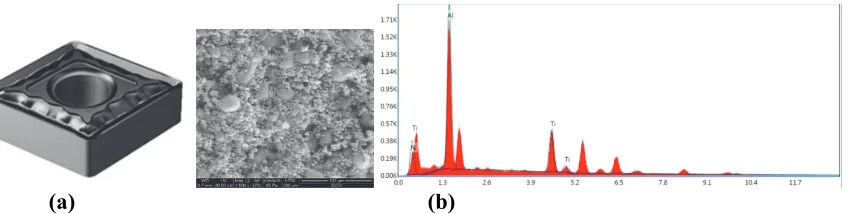
A cutting tool insert with ISO designation CNMG 120408-QM-1105 PVD TiAlN was used for the turning experiments. Fig. 3 also shows the photographic view of TiAlN insert, surface morphology and EDAX profile of PVD TiAlN insert. The Vickers hardness is 3100 HV.
(a) (b)
Fig. 3. Photographic view of (a) PVD TiAlN insert (b) Surface morphology and EDAX profile of PVD
TiAlN coating
3.3 Machining tests
All the machining experiments were conducted on ACE CNC LATHE JOBBER XL, with FANUC Oi Mate- TC as a controller. During the experiments, the combinations of the machining process parameter values were designed by using L36 mixed orthogonal array design of experiment. The cutting speeds were set at 50, 65 and 80 m/min, while the feed were 0.08, 0.15 and 0.2 mm/rev. The depth of cut was 0.5 mm is constant during the machining process. The machining experiments were carried out in MQL environment. The cutting conditions are shown in Table 2.
S. Nipanikar et al. Table 2
Cutting condition for experimental works
Machine tool ACE CNC LATHE JOBBER XL, FANUC Oi Mate- TC as a controller
Workpiece Material Titanium alloy, Ti-6Al-4V ELI
Cutting tool (insert) Cutting insert : Uncoated Carbide insert, ISO CNMG
120408-QM-1105 Sandvik make PVD TiAlN insert,
Tool holder PCLNL 2525 M12
Machining parameters Cutting speed (Vc): 50, 65 and 80 m/min
Feed (f): 0.08, 0.15 and 0.2 mm/rev Depth of cut (d): 0.5mm
Machining Environment MQL
Cutting Fluid Coconut oil ( Viscosity: 80 cP ), Palm oil (Viscosity:130 cP)
Cutting fluid supply For MQL cooling: air:6 bar, flow rate 54 ml/hr (through external
nozzle)
Turning parameters and their levels are shown in Table 3
Table 3
Turning Parameters and their levels
Machining Parameters Level 1 Level 2 Level 3
Cutting speed, Vc ( m/min ) 50 65 80
Feed, f (mm/rev) 0.08 0.15 0.2
Cutting tool, Ct Coated (PVD TiAlN) Uncoated --
Cutting fluid Palm oil Coconut oil --
Experimental Design layout is shown in Table 4.
Table 4
Experimental Design layout
Expt.
No. Environment Cutting Tool Insert Cutting
Cutting speed (m/min)
Feed
(mm/rev) Expt. No. Environment Cutting
Cutting Tool Insert Cutting speed (m/min) Feed (mm/rev) 1 MQL
(Palm Oil) Coated
50 0.08 19
MQL (Coconut
Oil)
Coated
50 0.08
2 50 0.15 20 50 0.15
3 50 0.2 21 50 0.2
4 65 0.08 22 65 0.08
5 65 0.15 23 65 0.15
6 65 0.2 24 65 0.2
7 80 0.08 25 80 0.08
8 80 0.15 26 80 0.15
9 80 0.2 27 80 0.2
10
MQL
(Palm Oil) Uncoated
50 0.08 28
MQL (Coconut
Oil) Uncoated
50 0.08
11 50 0.15 29 50 0.15
12 50 0.2 30 50 0.2
13 65 0.08 31 65 0.08
14 65 0.15 32 65 0.15
15 65 0.2 33 65 0.2
16 80 0.08 34 80 0.08
17 80 0.15 35 80 0.15
4. Results and discussions
4.1 Grey Relational Analysis
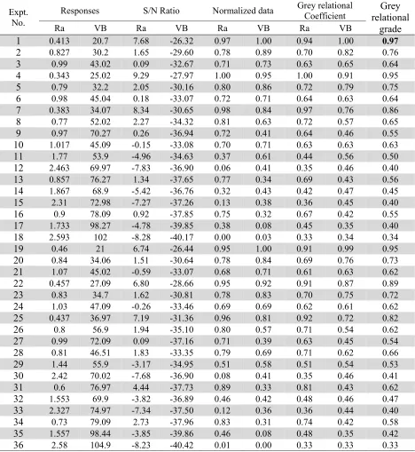
Initially, analysis and evaluation of single performance characteristic was performed. Then, multiple performance analysis were conducted by grey relational theory. From single performance analysis point of view the effect of machining parameters like cutting speed, feed rate, cutting tool insert and cutting fluid on the surface roughness and flank wear during turning of Ti6Al4V ELI in MQL environment was analyzed using response graphs which were drawn by using response table with the average values. The response table for surface roughness and tool flank wear is shown in Table 5.
Table 5
Observed response values, S/N ratio of responses, normalized values, grey relational coefficient and grey relational grade
Expt. No.
Responses S/N Ratio Normalized data Grey relational Coefficient Grey
relational grade
Ra VB Ra VB Ra VB Ra VB
1 0.413 20.7 7.68 -26.32 0.97 1.00 0.94 1.00 0.97
2 0.827 30.2 1.65 -29.60 0.78 0.89 0.70 0.82 0.76
3 0.99 43.02 0.09 -32.67 0.71 0.73 0.63 0.65 0.64
4 0.343 25.02 9.29 -27.97 1.00 0.95 1.00 0.91 0.95
5 0.79 32.2 2.05 -30.16 0.80 0.86 0.72 0.79 0.75
6 0.98 45.04 0.18 -33.07 0.72 0.71 0.64 0.63 0.64
7 0.383 34.07 8.34 -30.65 0.98 0.84 0.97 0.76 0.86
8 0.77 52.02 2.27 -34.32 0.81 0.63 0.72 0.57 0.65
9 0.97 70.27 0.26 -36.94 0.72 0.41 0.64 0.46 0.55
10 1.017 45.09 -0.15 -33.08 0.70 0.71 0.63 0.63 0.63
11 1.77 53.9 -4.96 -34.63 0.37 0.61 0.44 0.56 0.50
12 2.463 69.97 -7.83 -36.90 0.06 0.41 0.35 0.46 0.40
13 0.857 76.27 1.34 -37.65 0.77 0.34 0.69 0.43 0.56
14 1.867 68.9 -5.42 -36.76 0.32 0.43 0.42 0.47 0.45
15 2.31 72.98 -7.27 -37.26 0.13 0.38 0.36 0.45 0.40
16 0.9 78.09 0.92 -37.85 0.75 0.32 0.67 0.42 0.55
17 1.733 98.27 -4.78 -39.85 0.38 0.08 0.45 0.35 0.40
18 2.593 102 -8.28 -40.17 0.00 0.03 0.33 0.34 0.34
19 0.46 21 6.74 -26.44 0.95 1.00 0.91 0.99 0.95
20 0.84 34.06 1.51 -30.64 0.78 0.84 0.69 0.76 0.73
21 1.07 45.02 -0.59 -33.07 0.68 0.71 0.61 0.63 0.62
22 0.457 27.09 6.80 -28.66 0.95 0.92 0.91 0.87 0.89
23 0.83 34.7 1.62 -30.81 0.78 0.83 0.70 0.75 0.72
24 1.03 47.09 -0.26 -33.46 0.69 0.69 0.62 0.61 0.62
25 0.437 36.97 7.19 -31.36 0.96 0.81 0.92 0.72 0.82
26 0.8 56.9 1.94 -35.10 0.80 0.57 0.71 0.54 0.62
27 0.99 72.09 0.09 -37.16 0.71 0.39 0.63 0.45 0.54
28 0.81 46.51 1.83 -33.35 0.79 0.69 0.71 0.62 0.66
29 1.44 55.9 -3.17 -34.95 0.51 0.58 0.51 0.54 0.53
30 2.42 70.02 -7.68 -36.90 0.08 0.41 0.35 0.46 0.41
31 0.6 76.97 4.44 -37.73 0.89 0.33 0.81 0.43 0.62
32 1.553 69.9 -3.82 -36.89 0.46 0.42 0.48 0.46 0.47
33 2.327 74.97 -7.34 -37.50 0.12 0.36 0.36 0.44 0.40
34 0.73 79.09 2.73 -37.96 0.83 0.31 0.74 0.42 0.58
35 1.557 98.44 -3.85 -39.86 0.46 0.08 0.48 0.35 0.42
S. Nipanikar et al.
Table 5 shows higher grey relational grade for experiment number 1 i.e. optimum set of machining parameters. Optimal cutting condition is as follows.
Vc: 50 m/min f: 0.08 mm/rev., Ct: PVD TiAlN cutting fluid: Palm oil.
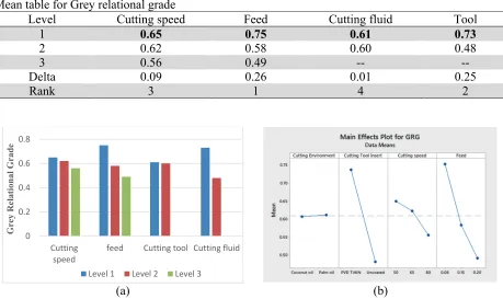
Mean table for grey relational grade is shown in Table 6. Effect of process parameters on grey relational grade is shown in Fig. 5. In the grey relational analysis, to obtain better performance a greater grey relational grade is required. From Table 6 and Fig. 5, the optimum machining parameter combination is determined as Vc: 50 m/min, f: 0.08 mm/rev., Ct: PVD TiAlN, cutting fluid: Palm oil for simultaneously achieving minimum surface roughness and minimum flank wear.
Fig. 4(a) indicates the grey relational grade of various levels of machining process parameters. It shows that the first level of each machining parameter indicates the highest grey relational grade. Feed was the dominant factor influencing the surface roughness and flank wear, simultaneously. Fig. 4(b) shows the main effect plots for grey relational grade.
Table 6
Mean table for Grey relational grade
Level Cutting speed Feed Cutting fluid Tool
1 0.65 0.75 0.61 0.73
2 0.62 0.58 0.60 0.48
3 0.56 0.49 -- --
Delta 0.09 0.26 0.01 0.25
Rank 3 1 4 2
(a) (b)
Fig. 4. (a) Effect of process parameters on grey relational grade and (b) Main effect plot for GRG
4.2 TOPSIS
The two response parameters such as surface roughness Ra and tool flank wear VB are normalized. In this article the same priority is given to both the responses i.e. surface roughness and flank wear weight are taken as 0.5 (i.e. WRa= 0.5 and WVB = 0.5). With the proper weight criteria the relative normalized weight matrix has been calculated. The weight criteria are multiplied to get the normalized weighted matrix using Eq. (6). The ideal and the negative ideal solutions are calculated from the normalized weighted matrix table. The separation measures of each criterion from the ideal and negative ideal solutions were calculated with Eqs. (7-8). Finally, the relative closeness coefficient (CCi) value for each combination of factors of turning process is calculated using Eq. (9). It was understood that the
0 0.2 0.4 0.6 0.8
Cutting speed
feed Cutting tool Cutting fluid
Grey
Rela
tion
al
Grad
e
experiment number 1 is the best experiment. Table 7 shows the normalized, weighted normalized data, separation measures and closeness coefficient.
Table 7
Normalized, weighted normalized data, Separation measures and Closeness coefficient values
Exp. No. Normalized data Weighted normalized data Separation measures coefficient Closeness
Ra VB Ra VB S+ S- CCi
1 0.05017 0.05558 0.02509 0.02779 0.00425 0.17410 0.97616
2 0.10046 0.08108 0.05023 0.04054 0.03205 0.14684 0.82086
3 0.12027 0.11550 0.06013 0.05775 0.04942 0.12799 0.72144
4 0.04167 0.06717 0.02083 0.03359 0.00580 0.17371 0.96769
5 0.09597 0.08645 0.04798 0.04323 0.03123 0.14669 0.82446
6 0.11905 0.12093 0.05953 0.06046 0.05064 0.12671 0.71446
7 0.04653 0.09147 0.02326 0.04574 0.01811 0.16450 0.90082
8 0.09354 0.13967 0.04677 0.06983 0.04940 0.13153 0.72696
9 0.11784 0.18866 0.05892 0.09433 0.07667 0.10899 0.58704
10 0.12355 0.12106 0.06177 0.06053 0.05242 0.12494 0.70444
11 0.21502 0.14471 0.10751 0.07236 0.09746 0.08477 0.46518
12 0.29921 0.18786 0.14960 0.09393 0.14476 0.04755 0.24726
13 0.10411 0.20477 0.05205 0.10239 0.08087 0.11223 0.58121
14 0.22680 0.18499 0.11340 0.09249 0.11294 0.06542 0.36679
15 0.28062 0.19594 0.14031 0.09797 0.13856 0.04617 0.24992
16 0.10933 0.20966 0.05467 0.10483 0.08414 0.10895 0.56423
17 0.21053 0.26384 0.10526 0.13192 0.13406 0.05299 0.28329
18 0.31500 0.27385 0.15750 0.13693 0.17490 0.00389 0.02177
19 0.05588 0.05638 0.02794 0.02819 0.00712 0.17167 0.96019
20 0.10204 0.09145 0.05102 0.04572 0.03511 0.14276 0.80259
21 0.12998 0.12087 0.06499 0.06044 0.05492 0.12255 0.69056
22 0.05552 0.07273 0.02776 0.03637 0.01102 0.16656 0.93792
23 0.10083 0.09316 0.05041 0.04658 0.03505 0.14265 0.80277
24 0.12512 0.12643 0.06256 0.06321 0.05474 0.12262 0.69137
25 0.05309 0.09926 0.02654 0.04963 0.02258 0.15958 0.87607
26 0.09718 0.15277 0.04859 0.07638 0.05596 0.12654 0.69335
27 0.12027 0.19355 0.06013 0.09678 0.07940 0.10687 0.57374
28 0.09840 0.12487 0.04920 0.06244 0.04478 0.13369 0.74910
29 0.17493 0.15008 0.08747 0.07504 0.08169 0.09608 0.54049
30 0.29398 0.18799 0.14699 0.09400 0.14248 0.04799 0.25196
31 0.07289 0.20665 0.03644 0.10333 0.07713 0.12673 0.62164
32 0.18866 0.18767 0.09433 0.09384 0.09881 0.07873 0.44344
33 0.28268 0.20128 0.14134 0.10064 0.14082 0.04331 0.23520
34 0.08868 0.21234 0.04434 0.10617 0.08183 0.11834 0.59120
35 0.18915 0.26430 0.09457 0.13215 0.12778 0.06352 0.33205
36 0.31342 0.28164 0.15671 0.14082 0.17674 0.00079 0.00445
From Table 7 it was understood that the experiment number 1 is the best experiment among the 36 experiment because this experiment shows the maximum closeness coefficient considering both responses and experiment number 36 shows the poor performance because it shows the lowest closeness coefficient among the 36 experiments. From Table 7, the optimum machining parameter combination determined as Vc: 50 m/min, f: 0.08 mm/rev., Ct: PVD TiAlN, cutting fluid: Palm oil for simultaneously achieving minimum surface roughness and minimum flank wear.
4.3 Response Surface Analysis
4.3.1 Surface roughness, Ra (µm)
S. Nipanikar et al.
Fig. 7 and Fig. 8 show the effect of the feed rate at various cutting speeds on the surface roughness. It is realized that surface roughness increases with an increase in the feed rate. The surface roughness is observed to be minimum at high cutting speed with low feed rate. Increasing feed rate, leading to vibration and generating more heat and consequently contributing to a higher surface roughness. Surface roughness decreases abruptly with the increase in cutting speed for a given value of feed rate. This is owing to the fact that, as cutting speed increases, the temperature increases at the cutting zone which leads to the tempering of material and thus reduces the surface roughness. Application of the cutting fluid at cutting zone decreases the coefficient of friction at the interface of the tool-chip over the rake face which gets better surface finish. The analysis of variance (ANOVA) was applied to study the effect of the machining process parameters on the surface roughness. Table 8 gives the statistical model summary of linear and quadratic model for Ra. It reveals that the quadratic model is the best model. So, for further investigation quadratic model was used.
Table 8
Model summary statistics for Ra
Source Standard deviation R2 Adj. R2
Linear model 0.160356 88.46 % 86.08 %
Quadratic model 0.150838 98.79 % 98.15 % suggested
Table 9 gives the response surface regression of surface roughness. The value ‘p’ i.e. probability of obtaining a result equal to or more extreme than what was actually observed. If ‘p’ value for the model is less than 0.05 which shows that the model terms are important. In order to understand the turning process, the experimental results were used to develop the second order model using response surface methodology (RSM). MINITAB 17 was used for the statistical analysis of experimental results. The proposed quadratic model was developed from the functional relationship using RSM method for following conditions separately. When, cutting tool: PVD TiAlN, cutting fluid: Coconut oil
Ra = 1.321 - 0.0311 Vc + 0.68 f + 0.000199 Vc*Vc + 9.47 f*f+ 0.0304 Vc*f (11) When, cutting tool: Uncoated, cutting fluid: Coconut oil
Ra = 0737- 0.0288 Vc + 9.20 f + 0.000199 Vc*Vc + 9.47 f*f+ 0.0304 Vc*f (12)
When, cutting tool: PVD TiAlN, cutting fluid: Palm oil
Ra = 1.430 - 0.0321 Vc + 0.04 f + 0.000199 Vc*Vc + 9.47 f*f+ 0.0304 Vc*f (13)
When, cutting tool: Uncoated, cutting fluid: Coconut oil
Ra = 1.061 - 0.0298 Vc + 8.56 f + 0.000199 Vc*Vc + 9.47 f*f+ 0.0304 Vc*f (14)
Table 9
Response surface design for Surface Roughness (Ra)
Source DF Adj SS Adj MS F P
Vc 1 0.0005 0.00053 0.06 0.807
f 1 7.3882 7.38816 841.70 0.000
Ct 1 6.7602 6.76023 770.16 0.000
Cutting fluid 1 0.0325 0.03246 3.70 0.067
Vc × Vc 1 0.0161 0.01605 1.83 0.189
f × f 1 0.0087 0.00870 0.99 0.330
Vc × f 1 0.0121 0.01207 1.37 0.253
Vc × Ct 1 0.0075 0.00746 0.85 0.366
Vc × Cutting fluid 1 0.0014 0.00143 0.16 0.691
f ×Ct 1 1.5812 1.58123 180.14 0.000
f ×Cutting fluid 1 0.0089 0.00894 1.02 0.324
Ct ×Cutting fluid 1 0.1047 0.10465 11.92 0.002
Error 23 0.2019 0.00878
Table 10
Analysis of variance for Ra
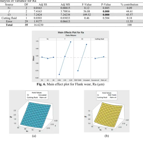
Source DF Adj SS Adj MS F-Value P-Value % contribution
Vc 2 0.0163 0.00815 0.12 0.885 0.09
f 2 7.4163 3.70816 56.08 0.000 44.61
Ct 1 7.2424 7.24238 109.52 0.000 43.57
Cutting fluid 1 0.0303 0.03033 0.46 0.504 0.18
Error 29 1.9177 0.06613 11.55
Total 35 16.6230 100
Fig. 6. Main effect plot for Flank wear, Ra (µm)
(a) (b)
Fig. 7. Surface plot of Ra in MQL enivironment (Palm oil ) (a) Unoated (b) PVD TiAlN insert
(a) (b)
S. Nipanikar et al.
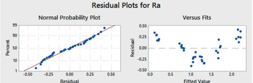
The acceptability of the model has been investigated by the examination of residuals. The residuals, which are the variance between the observed output and the predicted output are examined using normal probability plots of the residuals and the plots of the residuals versus the predicted response. If the model is aceptable, the points on the normal probability plots of the residuals should form a straight line. The plots of the residual versus the predicted response should be structureless, they should contain no noticeable pattern. The normal probability plots of the residuals and the plots of the residuals versus the predicted response for the surfac roughness values are shown in Fig. 9. It reveales that the residuals generally fall on a straight line indicating that the errors are distributed normally.
Fig. 9. Normal probability plot of residual and Plot of residual vs. fitted surface roughness values
4.3.2 Flank wear, VB (µm)
The cutting tool inserts in turning generally fail by gradual wear by abrasion, diffusion, adhesion, galvanic action and chemical erosion etc. depending on the workpiece and tool material and machining conditions. Tool wear initially starts with a relatively faster rate because of attrition and micro chipping at the sharp cutting edges. Cutting tools often fail prematurely, randomly and catastrophically by mechanical breakage and plastic deformation under adverse machining conditions caused by intensive pressure, temperature, dynamic loading at the tool tips if the tool material lacks strength, fracture toughness and hot hardness.
Fig. 11 and Fig. 12 show that flank wear increases with an increase in the cutting speed and feed rate. The flank wear is found to be minimum at low cutting speed with low feed rate. Increasing feed rate, leading to vibration and generating more heat and consequently contributing to a high flank wear. Flank wear increases abruptly with the increase in cutting speed. This is owing to the fact that, as cutting speed increases, the temperature increases at the cutting zone because Ti6Al4V ELI having low thermal conductivity (6.7 W/m-K). Due to the high temperature at the cutting zone, the tool loose its strength and thus plastic deformation took place. Application of the cutting fluid at cutting zone reduces the temperature through heat convection. As a result it leads to reduction in tool wear.
The analysis of variance (ANOVA) was applied to study the effect of the machining process parameters on the flank wear. Table 11 gives the statistical model summary of linear and quadratic model for VB. It reveals that the quadratic model is the best model. So, for further investigation quadratic model was used.
Table 11
Model summary statistics for VB
Source Standard deviation R2 Adj. R2
Linear model 0.160356 93.04 % 91.60 %
Table 12 gives the response surface regression of flank wear. The proposed quadratic model was developed from the functional relationship using RSM method for following conditions separately.
When, cutting tool: PVD TiAlN, cutting fluid: Coconut oil
VB = 80.5 - 2.36 Vc - 93 f + 0.02153 Vc×Vc + 657 f×f + 1.99 Vc×f (15)
When, cutting tool: Uncoated, cutting fluid: Coconut oil
VB = 93.9 - 1.85 Vc - 182 f + 0.02153 Vc×Vc + 657 f×f + 1.99 Vc×f (16)
When, cutting tool: PVD TiAlN, cutting fluid: Palm oil
VB = 80.1 - 2.38 Vc - 97 f + 0.02153 Vc×Vc + 657 f×f + 1.99 Vc×f (17)
When, cutting tool: Uncoated, cutting fluid: Palm oil
VB = 94.7 - 1.88 Vc - 186 f + 0.02153 Vc×Vc + 657 f×f + 1.99 Vc×f (18)
Table 12
Response surface design for Flank Wear (VB)
Source DF Adj SS Adj MS F P
Vc 1 4946.2 4946.2 142.41 0.000
f 1 2614.6 2614.6 75.28 0.000
Ct 1 10631.1 10631.1 306.09 0.000
Cutting fluid 1 30.8 30.8 0.89 0.356
Vc × Vc 1 187.7 187.7 5.40 0.029
f × f 1 41.9 41.9 1.21 0.283
Vc × f 1 51.8 51.8 1.49 0.234
Vc × Ct 1 345.6 345.6 9.95 0.004
Vc × Cutting fluid 1 0.7 0.7 0.02 0.890
f × Ct 1 173.4 173.4 4.99 0.035
f ×Cutting fluid 1 0.4 0.4 0.01 0.920
Ct × Cutting fluid 1 3.5 3.5 0.10 0.755
Error 23 798.8 34.7
Total 35 19744.5
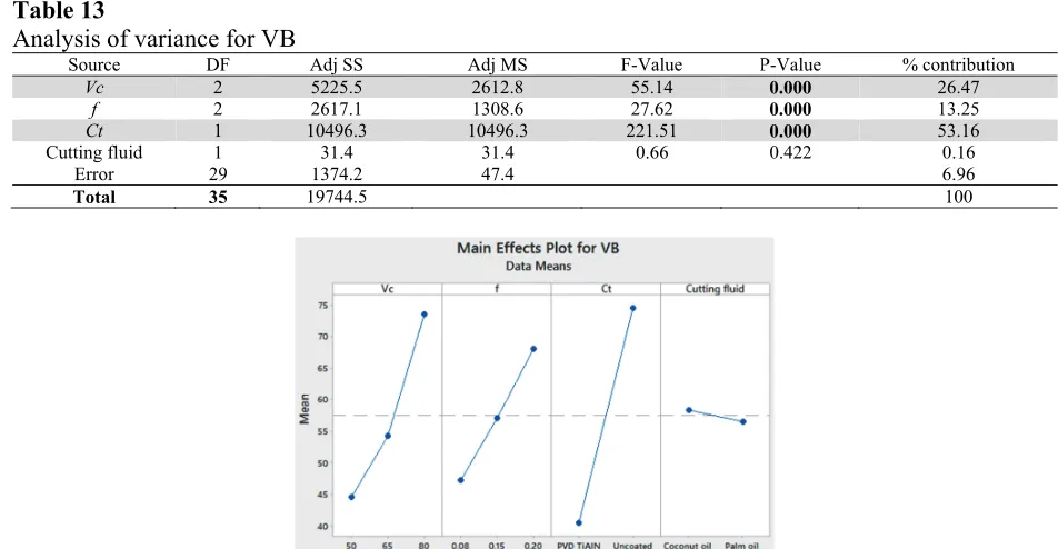
Table 13
Analysis of variance for VB
Source DF Adj SS Adj MS F-Value P-Value % contribution
Vc 2 5225.5 2612.8 55.14 0.000 26.47
f 2 2617.1 1308.6 27.62 0.000 13.25
Ct 1 10496.3 10496.3 221.51 0.000 53.16
Cutting fluid 1 31.4 31.4 0.66 0.422 0.16
Error 29 1374.2 47.4 6.96
Total 35 19744.5 100
S. Nipanikar et al.
(a) (b)
Fig. 11. Surface plot of VB in MQL enivironment (Palm oil ) (a) Unoated (b) PVD TiAlN insert
(a) (b)
Fig. 12. Surface plot of VB in MQL enivironment (Coconut oil ) (a) Unoated (b) PVD TiAlN insert
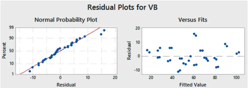
The normal probability plots of the residuals and the plots of the residuals versus the predicted response for the flank wear values are shown in Fig. 13. It reveales that the residuals usually fall on a straight line indicating that the errors are distributed normally.
Fig. 13. Normal probability plot of residual and Plot of residual vs. fitted flank wear values
are 0.94 and 0.96 for surface roughness and flank wear, respectively. So it is clear that the second order model is the most reliable.
(a) (b)
Fig. 14. Comparison of measured and predicted (a) surface roughness, Ra (µm) (b) Flank wear, VB
(µm) 4.4 Optimization of Response
The aim of experiments related to machining is to achieve the desired surface finish and minimum flank wear of cutting tool insert with the optimal cutting parameters. To attain this end, the RSM optimization seems to be a useful technique. The goal is to minimize surface roughness (Ra) and minimize flank wear (VB).
Fig. 15. Response Optimization for Surface roughness (Ra) and flank wear (VB)
Table 14
Confirmation test Sr.
No. Optimum Condition
Experimental Ra (
µ
m
)
R
SM Predicted Ra, (
µ
m)
Experimental VB (µm) RSM Predicted VB, (
µ
m
)
Vc
(m/min) f (mm/rev)
Cutting tool insert
Cutting fluid
1 60.3030 0.08 PVD TiAlN Palm oil 0.37 0.43 23.7 20.92
PVD TiAlN tool wear pattern is observed under scanning electron microscope at constant cutting speed of 80 m/min and at 0.08, 0.15 and 0.2 mm/rev feed under dry and minimum quantity lubrication environment. 0 0.5 1 1.5 2 2.5 3
3 5 7 9 11131517192123252729313335
su rfac e Rough n es s (Ra)
Experimental Run
Experimental Ra
0 20 40 60 80 100 120
1 3 5 7 9 11131517192123252729313335
Fla n k We ar (VB)
Experimental Run
S. Nipanikar et al. Cutting
condition
Dry MQL
Vc: 80 m/min, f: 0.08 mm/rev,
ap:0.5 mm
Vc: 80 m/min, f: 0.15 mm/rev,
ap: 0.5 mm
Vc: 80 m/min, f: 0.2 mm/rev,
ap: 0.5 mm
Fig. 16. SEM images of tool wear pattern for PVD TiAlN coated insert
5. Conclusions
The following can be concluded from the results obtained when turning of titanium alloy Ti-6Al-4V ELI under MQL environment using PVD TiAlN cutting tool:
Feed rate has the highest influence on the surface roughness and accounts for 44.61% contribution in the total variability of the model followed by cutting tool insert 43.57%.
Cutting tool has the highest influence on the flank wear and accounts for 53.16 % contribution in the total variability of the model followed by cutting speed insert 26.47%.
From the Grey relational analysis and TOPSIS method, the optimum combination of process parameters are considered as Vc: 50m/min, f: 0.08 mm/rev., Ct: PVD TiAlN, Cutting fluid: Palm oil
The optimum cutting process parameters were obtained through RSM as Vc: 60.3030 m/min, f: 0.08 mm/rev., Ct: PVD TiAlN and cutting fluid: Palm oil
Developed second order model has high square values of the regression coefficients which indicated high correlation with variances in the predictor values.
References
Ali, S. M., Dhar, N. R., & Dey, S. K. (2011). Effect of minimum quantity lubrication (MQL) on cutting performance in turning medium carbon steel by uncoated carbide insert at different speed-feed combinations. Advances in Production Engineering & Management, 6(3).
Attanasio, A., Gelfi, M., Giardini, C., & Remino, C. (2006). Minimal quantity lubrication in turning: effect on tool wear. Wear, 260(3), 333-338.
Dhar, N. R., Islam, S., & Kamruzzaman, M. (2007). Effect of minimum quantity lubrication (MQL) on tool wear, surface roughness and dimensional deviation in turning AISI-4340 steel. Gazi University Journal of Science,20(2), 23-32.
Escamilla-Salazar, I. G., Torres-Treviño, L. M., González-Ortíz, B., & Zambrano, P. C. (2013). Machining optimization using swarm intelligence in titanium (6Al 4V) alloy. The International Journal of Advanced Manufacturing Technology, 67(1-4), 535-544.
Islam, M. N., Anggono, J. M., Pramanik, A., & Boswell, B. (2013). Effect of cooling methods on dimensional accuracy and surface finish of a turned titanium part. The International Journal of Advanced Manufacturing Technology, 69(9-12), 2711-2722.
Khan, M. M. A., Mithu, M. A. H., & Dhar, N. R. (2009). Effects of minimum quantity lubrication on turning AISI 9310 alloy steel using vegetable oil-based cutting fluid. Journal of materials processing Technology, 209(15), 5573-5583.
Khanna, N., & Davim, J. P. (2015). Design-of-experiments application in machining titanium alloys for aerospace structural components. Measurement, 61, 280-290.
Liu, Z., An, Q., Xu, J., Chen, M., & Han, S. (2013). Wear performance of (nc-AlTiN)/(a-Si 3 N 4) coating and (nc-AlCrN)/(a-Si 3 N 4) coating in high-speed machining of titanium alloys under dry and minimum quantity lubrication (MQL) conditions. Wear, 305(1), 249-259.
Ramana, M. V., Vishnu, A. V., Rao, G. K. M., & Rao, D. H. (2012). Experimental Investigations, Optimization Of Process Parameters And Mathematical Modeling In Turning Of Titanium Alloy Under Different Lubricant Conditions. Journal of Engineering (IOSRJEN) www. iosrjen. org ISSN, 2250, 3021.
Revankar, G. D., Shetty, R., Rao, S. S., & Gaitonde, V. N. (2014). Analysis of surface roughness and hardness in titanium alloy machining with polycrystalline diamond tool under different lubricating modes. Materials Research, (AHEAD), 1010-1022.
Sargade, V., Nipanikar, S., & Meshram, S. (2016). Analysis of surface roughness and cutting force during turning of Ti6Al4V ELI in dry environment. International Journal of Industrial Engineering Computations, 7(2), 257-266.
Sharma, V. S., Singh, G., & Sørby, K. (2015). A review on minimum quantity lubrication for machining processes. Materials and Manufacturing Processes, 30(8), 935-953.
Shetty, R., Jose, T. K., Revankar, G. D., Rao, S. S., & Shetty, D. S. (2014). Surface Roughness Analysis during Turning of Ti-6Al-4V under Near Dry Machining using Statistical Tool. International Journal of Current Engineering and Technology, 4(3), 2061-2067.
Wang, P., Zhu, Z., & Wang, Y. (2016). A novel hybrid MCDM model combining the SAW, TOPSIS and GRA methods based on experimental design. Information Sciences, 345, 27-45.
Wu, H., & Guo, L. (2014). Machinability of titanium alloy TC21 under orthogonal turning process. Materials and Manufacturing Processes, 29(11-12), 1441-1445.
Xu, J. Y., Liu, Z. Q., An, Q. L., & Chen, M. (2012, April). Wear Mechanism of High-Speed Turning Ti-6Al-4V with TiAlN and AlTiN Coated Tools in Dry and MQL Conditions. In Advanced Materials Research (Vol. 497, pp. 30-34)