Mapping and assessing variability in the Antarctic marginal ice zone, pack ice and coastal polynyas in two sea ice algorithms with implications on breeding success of snow petrels

(1)

www.the-cryosphere.net/10/1823/2016/ doi:10.5194/tc-10-1823-2016

Mapping and assessing variability in the Antarctic marginal ice

zone, pack ice and coastal polynyas in two sea ice algorithms with

implications on breeding success of snow petrels

Julienne C. Stroeve1,2, Stephanie Jenouvrier3,4, G. Garrett Campbell1, Christophe Barbraud4, and Karine Delord4 1_{National Snow and Ice Data Center, Cooperative Institute for Research in Environmental Sciences,}

University of Colorado, Boulder, CO, USA

2_{Center for Polar Observation and Modelling, University College London, London, UK} 3_{Biology Department MS-34, Woods Hole Oceanographic Institution, Woods Hole, MA, USA} 4_{Centre d’Etudes Biologiques de Chizé, UMR 7372 CNRS, 79360 Villiers en Bois, France}

Correspondence to:Julienne C. Stroeve ([email protected])

Received: 28 January 2016 – Published in The Cryosphere Discuss.: 25 February 2016 Revised: 27 June 2016 – Accepted: 16 July 2016 – Published: 22 August 2016

Abstract. Sea ice variability within the marginal ice zone (MIZ) and polynyas plays an important role for phytoplank-ton productivity and krill abundance. Therefore, mapping their spatial extent as well as seasonal and interannual vari-ability is essential for understanding how current and future changes in these biologically active regions may impact the Antarctic marine ecosystem. Knowledge of the distribution of MIZ, consolidated pack ice and coastal polynyas in the total Antarctic sea ice cover may also help to shed light on the factors contributing towards recent expansion of the Antarctic ice cover in some regions and contraction in oth-ers. The long-term passive microwave satellite data record provides the longest and most consistent record for assessing the proportion of the sea ice cover that is covered by each of these ice categories. However, estimates of the amount of MIZ, consolidated pack ice and polynyas depend strongly on which sea ice algorithm is used. This study uses two popular passive microwave sea ice algorithms, the NASA Team and Bootstrap, and applies the same thresholds to the sea ice con-centrations to evaluate the distribution and variability in the MIZ, the consolidated pack ice and coastal polynyas. Results reveal that the seasonal cycle in the MIZ and pack ice is gen-erally similar between both algorithms, yet the NASA Team algorithm has on average twice the MIZ and half the consol-idated pack ice area as the Bootstrap algorithm. Trends also differ, with the Bootstrap algorithm suggesting statistically significant trends towards increased pack ice area and no

sta-tistically significant trends in the MIZ. The NASA Team al-gorithm on the other hand indicates statistically significant positive trends in the MIZ during spring. Potential coastal polynya area and amount of broken ice within the consoli-dated ice pack are also larger in the NASA Team algorithm. The timing of maximum polynya area may differ by as much as 5 months between algorithms. These differences lead to different relationships between sea ice characteristics and bi-ological processes, as illustrated here with the breeding suc-cess of an Antarctic seabird.

1 Introduction

(2)

changes, affecting global weather patterns (e.g., Jaiser et al., 2012). Sea ice also has important implications for the entire polar marine ecosystem, including sea ice algae, phytoplank-ton, crustaceans, fish, seabirds, and marine mammals, all of which depend on the seasonal cycle of ice formation in win-ter and ice melt in summer. For example, sea ice melt strati-fies the water column, producing optimal light conditions for stimulating bloom conditions. Antarctic seabirds rely upon the phytoplankton bloom for their breeding success and sur-vival (e.g., Park et al., 1999).

In stark contrast to the Arctic, which is undergoing a pe-riod of accelerated ice loss (e.g., Stroeve et al., 2012; Ser-reze and Stroeve, 2015), the Antarctic is witnessing a modest increase in total sea ice extent (SIE) (Parkinson and Cava-lieri, 2012; Simmonds et al., 2015). Sea ice around Antarc-tica reached another record high extent in September 2014, recording a maximum extent of more than 20 million km2for the first time since the modern passive microwave satellite data record began in October 1978. This follows previous record maxima in 2012 and 2013 (Reid et al., 2015), resulting in an overall increase in Antarctic September sea ice extent of 1.1 % per decade since 1979. While the observed increase is statistically significant, Antarctica’s SIE is also highly vari-able from year to year and region to region (e.g., Maksym et al., 2012; Parkinson and Cavalieri, 2012; Stammerjohn et al., 2012). For example, around the West Antarctic Peninsula (WAP), there have been large decreases in sea ice extent and sea ice duration (e.g., Ducklow et al., 2012; Smith and Stam-merjohn, 2001), coinciding with rapid warming since 1950 (Ducklow et al., 2012).

The temporal variability of the circumpolar Antarctic sea ice extent is underscored by sea ice conditions in 2015 when the winter ice cover returned back to the 1981–2010 long-term mean. Also, recent sea ice assessments from early satel-lite images from the Nimbus program of the late 1960s in-dicate a similarly high but variable SIE to that observed over 2012–2014 (Meier et al., 2013b; Gallaher et al., 2014). Mapping of the September 1964 ice edge indicates that ice extent likely exceeded both the 2012 and 2013 record monthly-average maxima, at 19.7±0.3 million km2. This was followed in August 1966 by an extent estimated at 15.9±0.3 million km2, considerably smaller than the record low maximum extent of the modern satellite record (set in 1986). The circumpolar average also hides contrasting re-gional variability, with some regions showing either strong positive or negative trends with magnitudes equivalent to those observed in the Arctic (Stammerjohn et al., 2012). In short, interannual and regional variability in Antarctic sea ice is considerable, and while the current positive trend in cir-cumpolar averaged Antarctic sea ice extent is important, it is not unprecedented compared to observations from the 1960s and is not regionally distributed.

Several explanations have been put forward to explain the positive Antarctic sea ice trends. Studies point to anomalous short-term wind patterns that both grow and spread out the

ice, related to the strength of the Amundsen Sea low pres-sure (e.g., Turner et al., 2013; Reid et al., 2015; Holland and Kwok, 2012). Other studies suggest meltwater from the un-derside of floating ice surrounding the continent has risen to the surface and contributed to a slight freshening of the surface ocean (e.g., Bintanja et al., 2013). While these stud-ies have helped to better understand how the ice, ocean and atmosphere interact, 2012 to 2014 showed different regions and seasons contributing to the net positive sea ice extent, which has made it difficult to establish clear links and sug-gests that no one mechanism can explain the overall increase. While the reasons for the increases in total extent remain poorly understood, it is likely that these changes are not just impacting total sea ice extent but also the distribution of pack ice, the marginal ice zone (MIZ) and polynyas. The MIZ is a highly dynamic region of the ice cover, defined by the tran-sition between the open ocean and the consolidated pack ice. In the Antarctic, wave action penetrates hundreds of kilome-ters into the ice pack, resulting in small rounded ice floes from wave-induced fracture (Kohout et al., 2014). This in turn makes the MIZ region particularly sensitive to both at-mospheric and oceanic forcing, such that during quiescent conditions it may consist of a diffuse thin ice cover, with iso-lated thicker ice floes distributed over a large (hundreds of kilometers) area. During high on-ice wind and wave events, the MIZ region contracts to a compact ice edge with rafted ice pressed together in front of the solid ice pack. The smaller the ice floes, the more mobile they are, and large variability in ice conditions can be found in response to changing wind and ocean conditions. Polynyas on the other hand are open-water areas near the continental margins (e.g., Morales-Maqueda et al., 2004) that often remain open as a result of strong kata-batic winds flowing down the Antarctic Plateau. The winds continuously push the newly formed sea ice away from the continent, which influences the outer ice edge as well, thus contributing to the overall increase in total ice extent in spe-cific regions around the Antarctic continent where katabatic winds are persistent.

(3)

et al., 2007, and references therein) play important roles as well.

In this study we use the long-term passive microwave sea ice concentration data record to evaluate variability and trends in the MIZ, pack ice and polynyas from 1979 to 2014. A complication arises, however, as to which sea ice algo-rithm to use. There are at least a dozen algoalgo-rithms available, spanning different time periods, which give sea ice concen-trations that are not necessarily consistent with each other (see Ivanova et al. ( 2014, 2015) for more information). To complicate matters, different studies have used different sea ice algorithms to examine sea ice variability and attribution. For example, Hobbs and Raphael (2010) used the Had1SST1 sea ice concentration data set (Rayner et al., 2003), which is based on the NASA Team algorithm (Cavalieri et al., 1999), whereas Raphael and Hobbs (2014) relied on the Bootstrap algorithm (Comiso and Nishio, 2008). To examine the influ-ence in the choice of sea ice algorithm on the results, we use both the Bootstrap (BT) and NASA Team (NT) sea ice algorithms. Results are evaluated hemisphere-wide and also for different regions. We then discuss the different implica-tions resulting from the two different satellite estimates for biological impact studies. We focus on the breeding success of snow petrels because seabirds have been identified as use-ful indicators of the health and status of marine ecosystems (Piatt and Sydeman, 2007).

2 Data and methods

To map different ice categories, the long-term passive mi-crowave data record is used, which spans several satel-lite missions, including the Scanning Multichannel Mi-crowave Radiometer (SMMR) on the Nimbus-7 satellite (Oc-tober 1978 to August 1987) and the Special Sensor Mi-crowave Imager (SSM/I) sensors F8 (July 1987 to Decem-ber 1991), F11 (DecemDecem-ber 1991 to SeptemDecem-ber 1995) and F13 (May 1995 to December 2007) and the Special Sensor Mi-crowave Imager/Sounder (SSMIS) sensor F17 (January 2007 to present), both on the Defense Meteorological Satellite Program’s (DMSP) satellites. Derived sea ice concentrations (SICs) from both the Bootstrap (Comiso and Nishio, 2008) and the NASA Team (Gloersen et al., 1992; Cavalieri et al., 1999) are available from the National Snow and Ice Data Center (NSIDC) and provide daily fields from October 1978 to present, gridded to a 25 km polar stereographic grid. While a large variety of SIC algorithms are available, the lack of good validation has made it difficult to determine which al-gorithm provides the most accurate results during all times of the year and for all regions. Using two algorithms pro-vides a consistency check on variability and trends. Note that NSIDC has recently combined these two algorithms to build a climate data record (CDR) (Meier et al., 2013a).

Using these SIC fields, we define six binary categories of sea ice based on different SIC thresholds (Table 1).

Be-cause the marginal ice zone is highly dynamic in time and space, it is difficult to precisely define this region of the ice cover. Wadhams (1986) defined the MIZ as that part of the ice cover close enough to the open-ocean boundary to be im-pacted by its presence, e.g., by waves. Thus the MIZ is typ-ically defined as the part of the sea ice that is close enough to the open ocean to be heavily influenced by waves, and it extends from the open ocean to the dense pack ice. In this study, we define the MIZ as extending from the outer sea ice–open-ocean boundary (defined by SIC≥0.15 ice frac-tion) to the boundary of the consolidated pack ice (defined by SIC=0.80). This definition was previously used by Strong and Rigor (2013) to assess MIZ changes in the Arctic and matches the upper SIC limit used by the National Ice Center (NIC) in mapping the Arctic MIZ. The consolidated ice pack is then defined as the area south of the MIZ with ice fractions between 0.80≤SIC≤1.0. Potential coastal polynyas are de-fined as regions near the coast that have SIC < 0.80.

To automate the mapping of different ice categories, radial transects from 50 to 90◦S are individually selected to con-struct one-dimensional profiles (Fig. 1). The algorithm first steps from the outer edge until the 0.15 SIC is detected, pro-viding the latitude of the outer MIZ edge. Next, the algorithm steps from the outer MIZ edge until either the 0.80 SIC is encountered or the continent is reached. Data points along the transect between these SIC thresholds are flagged as the MIZ. In this way, the MIZ includes an outer band of low sea ice concentrations that surrounds a band of inner con-solidated pack ice, but sometimes the MIZ also extends all the way to the Antarctic coastline (as sometimes observed in summer). South of the MIZ, the consolidated ice pack (0.80≤SIC≤1.0) is encountered; however, low sea ice con-centrations can appear near the coast inside the pack ice re-gion as well. These are areas of potential coastal polynyas. While it is difficult to measure the fine-scale location of a polynya at 25 km spatial resolution, the lower sea ice con-centrations provide an indication of some open water near the coast, which for seabirds provides a source of open water for foraging. We have previously tested mapping polynyas using a SIC threshold of 0.75 and 0.85 for the NASA Team and Bootstrap algorithms, respectively, and found that these thresholds provided consistent polynya areas between the two algorithms and matched other estimates of the spatial distribution of polynyas (see Li et al., 2016). However, for this study we chose just one threshold, a compromise be-tween the two algorithms, so that we can better determine the sensitivity of using the same threshold on polynya area and timing of formation.

(4)

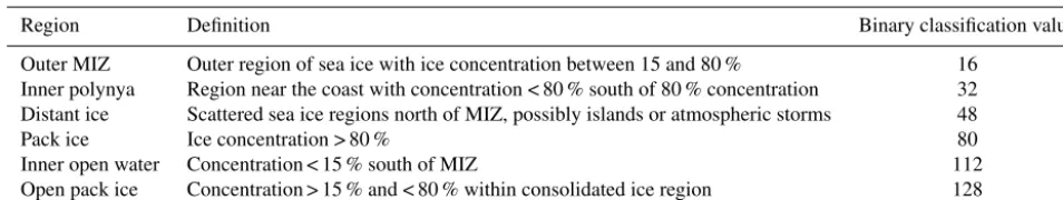
Table 1.Sea ice categories defined in this study.

Region Definition Binary classification value

Outer MIZ Outer region of sea ice with ice concentration between 15 and 80 % 16 Inner polynya Region near the coast with concentration < 80 % south of 80 % concentration 32 Distant ice Scattered sea ice regions north of MIZ, possibly islands or atmospheric storms 48

Pack ice Ice concentration > 80 % 80

Inner open water Concentration < 15 % south of MIZ 112

Open pack ice Concentration > 15 % and < 80 % within consolidated ice region 128

Figure 1.Example of a radial profile from 50 to 90◦S at−11.60◦W on 3 September 1990, showing the different sea ice classifications found along this transect.

within the consolidated pack ice, respectively. Finally, an ocean mask derived from climatology and distributed by NSIDC was applied to remove spurious ice concentrations at the ice edge as a result of weather effects.

Figure 2 shows sample images of the classification scheme as applied to the NASA Team and Bootstrap algorithms on days 70 (11 March) and 273 (30 September), respectively, in 2013. During the fall and winter months when the ice cover is expanding there is a well-established consolidated pack ice region, surrounded by the outer MIZ. Coastal polynyas are also found surrounding the continent in both algorithms. The BT algorithm tends to show a larger consolidated ice pack than NT, particularly during the timing of maximum extent. During the melt season there is mixing of low and high ice concentrations, leading to mixtures of different cat-egories, which is still seen to some extent in the March images. However, during March areas of polynyas (green), open water (pink) and open pack ice (orange) appear to ex-tend from the coastline in some areas (e.g., southern Weddell and Ross seas). While any pixel with SIC < 0.8 adjacent to the coastal boundary is flagged as potential polynya when stepping northwards, if a pixel is already flagged as MIZ or consolidated pack ice when stepping southwards, it remains flagged as MIZ or pack ice. After that analysis, a check for pixels with SICs less than 0.8 is done to flag for broken ice or open water. Thus, during these months (e.g., December to

Figure 2.Samples of ice classification on day 70 (March) and day 273 (September) 2013. Results are shown for both the NASA Team (top) and Bootstrap (bottom) sea ice algorithms. The MIZ (red) rep-resents regions of sea ice concentration between 15 and 80 % from the outer ice edge; the pack ice is shown in light purple, representing regions of greater than 80 % sea ice concentration. Orange regions within the pack ice represent coherent regions of less than 80 % sea ice concentration, pink areas open water and green regions of less than 80 % sea ice concentration near the Antarctic coastline. Dark blue represents the ocean mask applied to remove spurious ice con-centrations beyond the ice edge.

February or March), the physical interpretation of the differ-ent ice classes may be less useful.

(5)

Figure 3.Southern Hemisphere regions as defined by Parkinson and Cavalieri (2012).

classification together with the±1 standard deviation (1σ ). Monthly trends over the entire time series are computed by first averaging the daily fields into monthly values and then using a standard linear least squares, with statistical signifi-cance evaluated at the 90th, 95th and 99th percentiles using a Studentttest.

3 Results

3.1 Seasonal cycle 3.1.1 Circumpolar extent

We begin with an assessment of the consistency of the outer ice edge between both sea ice algorithms (Fig. 4). As a result of the large emissivity difference between open water and sea ice, estimates of the outer ice edge location have high consis-tency between the two algorithms despite having large differ-ences in SIC (e.g., Ivanova et al., 2014, 2015). This results in similar total sea ice extents between both algorithms during all calendar months, except for a small southward displace-ment of the Bootstrap ice edge during summer, and similar long-term trends. This is where the similarities end, however. Figure 5 summarizes the climatological mean seasonal cycle in the extent of the different ice categories listed in Table 1 for both sea ice algorithms, averaged for the total hemispheric-wide Antarctic sea ice cover. The 1 standard de-viation is given by the colored shading. The first notable re-sult is that the BT algorithm has a larger consolidated ice pack than the NT algorithm, which comes at the expense of a smaller MIZ. Averaged over the entire year, the NT MIZ area is twice as large as that from BT (see also Table 2). The BT algorithm additionally has a smaller spatial extent of poten-tial coastal polynyas and little to no broken ice or open water within the consolidated pack ice. Another important result is

Figure 4.Location of the mean 1981–2010 outer marginal ice edge for both the NASA Team and Bootstrap algorithms.

that the BT algorithm exhibits less interannual variability in the five ice categories identified, as illustrated by the smaller standard deviations from the long-term mean. Thus, while the total extents are not dissimilar between the algorithms, how that ice is distributed among the different ice categories differs quite substantially as well as their year-to-year vari-ability.

(6)

Figure 5.Long-term (1979–2013) and standard deviation (shading) of the seasonal cycle in total Antarctic extent of the consolidated pack ice, the outer marginal ice zone, polynyas, open pack ice (or broken ice within the pack ice), and inner open water. There are essentially no scattered ice floes outside of the MIZ. NASA Team results are shown on the left and the Bootstrap on the right.

(in November–December) as compared to the slow ice edge advance in autumn (see Watkins and Simmonds, 1999).

Open pack ice is negligible in the Bootstrap algorithm except for a slight peak in November/December. With the NASA Team algorithm, however, there is a clear increase in open pack ice during the ice expansion phase, which con-tinues to increase further as the pack ice begins to retreat, also peaking in November. Open pack ice in September con-tributes another 1.28×106km2to the total Antarctic sea ice extent in the NT algorithm, compared to only 0.36×106km2 in the BT algorithm. As with the open pack ice, the frac-tion of potential coastal polynyas also increases during the ice expansion phase; it then continues to increase as the sea ice retreats, peaking around November in the NT algorithm, with a total area of 1.02×106km2, and in December in BT (0.81×106km2). Inner open water within the pack is gener-ally only found between November and March in both algo-rithms as the total ice cover retreats and reaches its seasonal minimum.

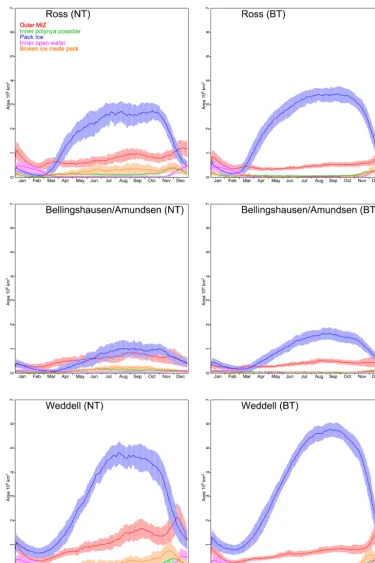
3.1.2 Regional analysis

Analysis of the Antarctica-wide sea ice cover, however, is of limited value given that the sea ice variability and trends are spatially heterogeneous (Maksym et al., 2012). For example, while the ice cover is increasing in the Ross Sea, it has at the same time decreased in the Bellingshausen–Amundsen (B– A) Sea region. Thus, we may anticipate significant regional variability in the amount, seasonal cycle and trends of the different ice classes (trends discussed in Sect. 3.3). The Ross Sea for example (Fig. 6, top) consists of a large fraction of consolidated ice throughout most of the year (April through November) in both algorithms, with considerably less MIZ. In the B–A Sea on the other hand (Fig. 6, 2nd row), the NT

algorithm has a MIZ extent that exceeds that of the consol-idated pack ice until May, after which the spread (±1σ) in MIZ and consolidated pack ice overlaps. The reverse is true in the BT algorithm, which consistently indicates a more consolidated ice pack, with only 0.51×106km2 flagged as MIZ during the maximum extent in September, compared to 0.84×106km2in the NT algorithm. On an annual basis, the NT algorithm shows about equal proportion of MIZ and con-solidated pack ice in the B–A Sea, whereas the BT algorithm indicates a little more than a third of the total ice cover is MIZ. Note also that the B–A Sea is the only region where the maximum MIZ extent does not occur after the maximum pack ice extent during spring. This is true for both sea ice algorithms.

In the Ross Sea there is also a very broad peak in the max-imum extent of the consolidated pack ice, stretching between July and October in the NT algorithm, and a peak in MIZ ex-tent in late August–early September with a secondary peak in December as the pack ice continues to retreat. The BT algo-rithm shows a similar broad peak in the pack ice extent, but with less interannual variability, and a nearly constant frac-tion of MIZ throughout the advance and retreat of the pack ice. Annually the NT algorithm shows about 56 % more MIZ in the Ross Sea than the BT algorithm. Note that in both algo-rithms the pack ice retreats rapidly after the maximum extent is reached.

(7)

Figure 6.

winds and currents. The open pack ice north of the pack ice continues to expand either by further freezing or breaking of the pack ice by the winds and currents. Overall, the Wed-dell Sea has the largest spatial extent in the MIZ in both

(8)

Figure 6.Long-term (1979–2013) seasonal cycle in regional sea ice extent of the consolidated pack ice, the outer marginal ice zone, polynyas, open pack ice (or broken ice within the pack ice), and inner open water. Results for the NASA Team algorithm are shown on the left and Bootstrap on the right for the Ross Sea, Bellingshausen–Amundsen Sea, Weddell Sea, Indian Ocean and Pacific Ocean.

NASA Team algorithm gives a climatological mean MIZ ex-tent of 1.61×106km2, twice as large as that in the Bootstrap algorithm (0.83×106km2).

Finally, in the Indian and Pacific Ocean sectors (Fig. 6, fourth row and bottom) the MIZ extent increases from March until November in both algorithms, retreating about a month after the peak extent in the pack ice is reached. However, in the Pacific Ocean sector, the NT MIZ comprises a larger per-centage of the overall ice cover, being nearly equal in spatial extent and even exceeding that of the pack ice in Septem-ber (0.93 (MIZ) vs. 0.76×106km2(pack ice)). This results in an annual mean extent of MIZ that exceeds that of the consolidated pack ice. This is the only region of Antarctica where this occurs. In the BT algorithm, the reverse is true, with again a larger annual extent of pack ice than MIZ.

While the above discussion focused on regional differ-ences in the MIZ and the consolidated pack ice, the spatial extent and timing of coastal polynyas also vary between the

(9)

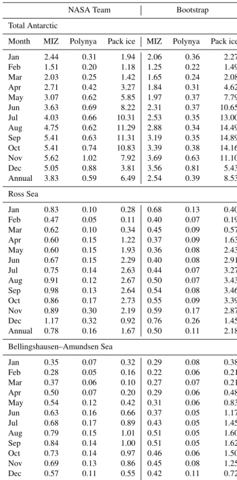
Table 2.Monthly-mean extents of the different ice classes. Values are only listed for the consolidated pack ice, the marginal ice zone and the potential coastal polynya area. Values are listed in 106km2.

NASA Team Bootstrap

Total Antarctic

Month MIZ Polynya Pack ice MIZ Polynya Pack ice

Jan 2.44 0.31 1.94 2.06 0.36 2.27 Feb 1.51 0.20 1.18 1.25 0.22 1.49 Mar 2.03 0.25 1.42 1.65 0.24 2.08 Apr 2.71 0.42 3.27 1.84 0.31 4.62 May 3.07 0.62 5.85 1.97 0.37 7.79 Jun 3.63 0.69 8.22 2.31 0.37 10.65 Jul 4.03 0.66 10.31 2.53 0.35 13.00 Aug 4.75 0.62 11.29 2.88 0.34 14.49 Sep 5.41 0.63 11.31 3.19 0.35 14.89 Oct 5.41 0.74 10.83 3.39 0.38 14.16 Nov 5.62 1.02 7.92 3.69 0.63 11.10 Dec 5.05 0.88 3.81 3.56 0.81 5.43 Annual 3.83 0.59 6.49 2.54 0.39 8.53

Ross Sea

Bellingshausen–Amundsen Sea

3.2 Trends

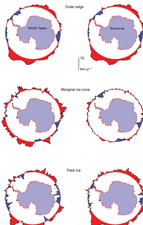
3.2.1 Spatial expansion–contraction during September As mentioned earlier, estimates of the outer ice edge loca-tion are similar between both algorithms. This is also true in terms of the locations where the outer edge is expanding or contracting. A way to illustrate this is shown in Fig. 7 (top), which shows a spatial map of the trend in the outer edge of

Table 2.Continued.

NASA Team Bootstrap

Total Antarctic

Month MIZ Polynya Pack ice MIZ Polynya Pack ice

Weddell Sea

Indian Ocean

Pacific Ocean

(10)

to-Figure 7.Expansion (red) or contraction (blue) of the outer ice edge (top), the width of the marginal ice zone (middle) and the width of the pack ice from 1979 to 2013 during the month of September.

wards contraction of the outer ice edge. The Bellingshausen and Weddell seas also show trends towards contraction of the outer ice edge.

While there is general consistency between the algorithms in both the location and changes of the outer ice edge over time, there are differences as to how the MIZ and pack ice widths are changing (Fig. 7, middle and bottom). The BT MIZ width is a relatively constant ring around the edge of the consolidated pack ice, with little change over time. Thus, in the BT algorithm, the spatial pattern of expansion– contraction of the total ice cover in September is largely a re-sult of the changes happening in the pack ice (Fig. 7, bottom). The NT algorithm on the other hand shows more pronounced changes in the MIZ, such that both the MIZ and the pack ice contribute to the observed spatial patterns and changes in the total ice cover. However, expansion–contraction of the NT MIZ and of the NT pack ice sometimes counteract each other. For example the contraction of the total ice edge of the

Bellingshausen Sea is a result of contraction of the consoli-dated ice pack, while the MIZ width is generally increasing as a result of the MIZ moving further towards the continent. This is also true in the Weddell Sea and the Indian Ocean.

Somewhat surprisingly, the spatial pattern of expansion– contraction of the MIZ is broadly similar between both algo-rithms, despite overall smaller changes in the BT algorithm. This highlights the fact that the spatial trends in SIC are similar to the spatial trends in SIE as well as to the timing of advance/retreat/duration, so that the spatial trends in the MIZ and pack ice will show the same overall pattern because they rely on SIC. This also highlights the fact that the spa-tial pattern persists throughout the regional ice-covered area, i.e., from the edge to the coastal area, which may imply that climate-related regional wind-driven changes at the ice edge are felt all the way to the coast. Alternatively it may imply that the ocean is also responding to the same climate-related wind changes, thus communicating the change all the way to the coast.

3.2.2 Circumpolar and regional daily trends

(11)

consis-tent between both algorithms, though the magnitudes of the trends tend to be larger in the Bootstrap algorithm. For ex-ample, in the Ross Sea, the sign of the pack ice trends are spatially consistent between both algorithms, though not all trends are statistically significant, particularly for the NT al-gorithm. The largest consistency occurs in the the western Ross Sea, where positive trends are seen in both algorithms, statistically significant from March to November (p< 0.01) in the BT algorithm, and from January to July and October to November in the NT algorithm. Note also that both al-gorithms show statistically significant positive trends in the MIZ from January to March in the western Ross Sea and generally negative trends in the eastern Ross Sea. This pat-tern switches from June to December, with mostly negative MIZ trends in the western Ross Sea and positive trends in the eastern Ross Sea. In particular, the statistically signifi-cant positive trends in the MIZ in the NT algorithm occur at the time of year with the largest overall trends in the SIE in this region. This would suggest perhaps different interpreta-tion of processes impacting the overall ice expansion in the Ross Sea depending on which algorithm is used.

In the B–A Sea, statistically significant positive trends in pack ice are limited to May through August in the NT algo-rithm and June and July in the BT algoalgo-rithm. The positive NT pack ice trends are offset by negative trends in the NT MIZ. Both algorithms exhibit negative pack ice trends dur-ing other months that are consistent between the algorithms, albeit larger in magnitude for the BT algorithm. This is gen-erally compensated for by statistically significant negative trends in the NT MIZ to give an overall negative decline of total extent.

Trends in the pack ice are also consistent between algo-rithms in the Weddell Sea, with statistically significant trends generally occurring at the same longitude and during the same months. The positive pack ice trends in MAM (NT) or MAMJ (BT) are confined to a very narrow longitude band which moves to the east with progressing season. Then in June, and continuing for several months, negative pack ice trends occur. For both algorithms, trends in the MIZ are gen-erally not statistically significant, except for some positive trends in the eastern Weddell Sea from January to March and negative trends mostly from June to November near 330◦ longitude.

Finally, in the Pacific and Indian oceans we again see spa-tial consistency in pack ice and MIZ trends for both algo-rithms, with generally larger (smaller) pack ice (MIZ) trends for the BT algorithm, though trends are closer in magnitude in the Pacific sector from March to July. Pack ice trends are generally positive, being more in BT than NT, and trends in MIZ extent basically vary around zero with exceptions dur-ing August through December in both algorithms in the Pa-cific Ocean.

In summary, while the magnitude of trends differs between both algorithms, there is general spatial consistency in the patterns of positive and negative trends in the consolidated

pack ice and the MIZ. Results suggest that positive trends in total SIE are generally a result of statistically significant pos-itive trends in the consolidated pack ice in the BT algorithm in all sectors of the Antarctic, except for the Bellingshausen– Amundsen Sea sector and the Weddell Sea during ice retreat. The NT algorithm on the other hand suggests more instances of statistically significant positive trends in the MIZ, though this is highly regionally dependent.

3.2.3 Seasonal trends in MIZ and pack ice width

Finally, we compute the overall width of the MIZ and pack ice following Strong and Rigor (2013) and produce seasonal means. Briefly, following the classification of each ice cat-egory, latitude boundaries are computed for each longitude and each day. These are averaged for each month to provide monthly-mean latitude boundaries at each longitude. The boundaries are subsequently converted to width in kilome-ters and averaged for all longitudes. Finally, seasonal means are derived.

Time series of seasonal means of the circumpolar MIZ width and pack ice width are shown in Fig. 10 for all sea-sons except summer, when the results are noisy. As we may expect following the previous results, the NT MIZ width is larger and the pack ice width is smaller than seen in the BT algorithm. During autumn (MAM), however, the differences in widths for both the MIZ and the pack ice between the al-gorithms are largely reduced compared to the other seasons. For example the difference in 1979–2013 pack ice width be-tween the algorithms is 60 km during MAM, 121 km during JJA and 139 km during SON. Similarly, the long-term mean MIZ width differences are 54 km (MAM), 74 km (JJA) and 83 km (SON). In addition, during autumn, trends in the MIZ and pack ice are largely consistent between the two algo-rithms, with no trend in the MIZ and increases in the pack ice on the order of 21.2 and 20.0 km decade−1(p< 0.01) for the BT and NT algorithms, respectively. This is the season with the largest trends in the pack ice width, representing a 21 % widening over the satellite record.

(12)

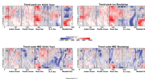
Figure 8.Daily trends (1979 to 2013) in the consolidated pack ice, the outer MIZ and potential coastal polynyas for the entire Antarctic sea ice cover for the NASA Team (left) and Bootstrap (right) algorithms. Trends are provided in 106km2yr−1.

Figure 9.Daily (1979–2013) trends in regional sea ice extent of the consolidated pack ice (top), the outer marginal ice zone (middle) and potential coastal polynyas (bottom). Results for the NASA Team algorithm (left) and Bootstrap (right) are shown as a function of longitude. Trends are provided in 106km2yr−1. Note the difference in color bar scales.

of expansion both equatorward and southwards, yet it is not statistically significant.

For the pack ice, both sea ice algorithms show statisti-cally significant positive trends towards increased width of the pack ice, which are also nearly identical during winter at

+18.7 and+18.1 km decade−1(p< 0.01) for the BT and NT

(13)

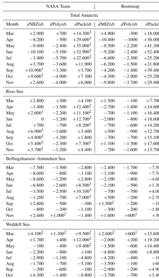
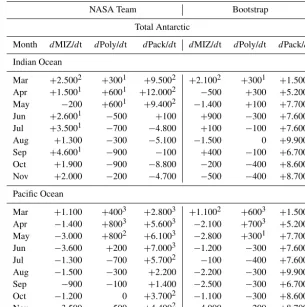
Table 3. Comparison of trends in the marginal ice zone, polynyas and the consolidated pack ice for March through November (1979 to 2013) for both the NASA Team and Bootstrap sea ice algorithms. Trends are computed in square kilometers per year (km2yr−1). Statistical significance at the 90th, 95th and 99th percentiles are denoted by 1, 2 and3, respectively. Results are only shown for March through November.

NASA Team Bootstrap

Total Antarctic

Month dMIZ/dt dPoly/dt dPack/dt dMIZ/dt dPoly/dt dPack/dt

Mar +2.900 +700 +14.3003 +4.900 -300 +18.0003 Apr −8.200 −500 +29.6003 −10.400 −1000 +38.0003

May −9.400 −2.400 +35.0003 −8.500 −2.200 +41.3003

Jun −10.100 −5.100 +32.9003 −9.200 −2.400 +52.4003

Jul −3.400 −5.700 +22.6002 −6.600 −2.300 +25.2003

Aug +3.700 −3.600 +11.900 −6.200 −1.500 +31.8003

Sep +10.9001 −3.300 +3.700 −4.200 −1.400 +39.4003

Oct +9.6001 −4.900 +7.300 −4.300 −2.900 +25.2003

Nov +2.600 −4.000 +6.000 −9.800 −3.700 +29.4003

Ross Sea

Mar +2.800 +300 +4.100 +1.500 −100 +7.7002 Apr −1.400 −1.500 +12.4002 −2.700 −1.400 +14.6003 May +2.6001 −2.200 +11.1002 −700 −1.100 +16.4003 Jun 0 −1.200 +12.7002 −2.000 −800 +18.6003 Jul +700 −700 +8.2001 −700 −600 +14.2003 Aug +6.9003 −1.600 +3.400 +500 −900 +12.7003 Sep +4.8002 −1.200 +1.800 −700 −700 +15.1003 Oct +5.4003 −2.300 +7.3001 +1.100 −1.300 +17.6003 Nov +3.7001 −1.200 +4.400 −700 −1.600 +13.7003

Bellingshausen–Amundsen Sea

Mar −7.500 −1.500 −2.800 −2.400 −1.700 −7.500

Apr −8.600 −800 −3.100 −3.100 −900 −7.700

May −8.600 −1.200 +2.800 −2.100 −800 −4.600 Jun −6.800 −2.600 +8.5003 −2.100 −500 +1.300 Jul −3.500 −2.500 +10.1003 −700 −700 +4.000 Aug −1.200 −700 +7.0001 +500 −200 +2.700

Sep +2.600 −500 −300 +1.5001 −200 −100

Oct −800 −200 −1.100 −300 −200 −1.800

Nov +2.600 +1.0002 −1.400 +1.600 +6001 +300

Weddell Sea

Mar +4.1002 +1.3002 +9.5002 +2.6002 +6001 +13.6003

Apr +1.700 +400 +12.0002 −2.000 +200 +19.2003

May −100 −400 +9.4002 −1.500 −600 +14.4003

Jun −2.300 −900 +100 −4.800 −600 +8.8002

Jul −2.900 −1.100 −4.800 −4.200 −400 −100

Aug −1.700 −700 −5.100 −3.500 −100 +600

Sep −200 −600 −100 −2.900 −200 +4.900

Oct +4.300 −1.400 −8.800 −3.700 −700 +3.400

Nov −2.100 −3.500 −4.700 −6.300 −2.200 +700

with trends of +10.0 (p< 0.05) km decade−1 compared to

+16.7 (p< 0.01) for the BT algorithm.

(14)

Table 3.Continued.

NASA Team Bootstrap

Total Antarctic

Month dMIZ/dt dPoly/dt dPack/dt dMIZ/dt dPoly/dt dPack/dt

Indian Ocean

Mar +2.5002 +3001 +9.5002 +2.1002 +3001 +1.5002 Apr +1.5001 +6001 +12.0002 −500 +300 +5.2003 May −200 +6001 +9.4002 −1.400 +100 +7.7003 Jun +2.6001 −500 +100 +900 −300 +7.6002 Jul +3.5001 −700 −4.800 +100 −100 +7.6002

Aug +1.300 −300 −5.100 −1.500 0 +9.9003

Sep +4.6001 −900 −100 +400 −100 +6.7002 Oct +1.900 −900 −8.800 −200 −400 +8.6002 Nov +2.000 −200 −4.700 −500 −400 +8.7002

Pacific Ocean

Mar +1.100 +4003 +2.8003 +1.1002 +6003 +1.5002

Apr −1.400 +8003 +5.6003 −2.100 +7003 +5.2003

May −3.000 +8002 +6.1003 −2.800 +3001 +7.7003

Jun −3.600 +200 +7.0003 −1.200 −300 +7.6002

Jul −1.300 −700 +5.7002 −100 −400 +7.6002

Aug −1.500 −300 +2.200 −2.200 −300 +9.9003

Sep −900 −100 +1.400 −2.500 −300 +6.7002

Oct −1.200 0 +3.7002 −1.100 −300 +8.6002

Nov −3.500 −500 +4.4002 −4.000 −200 +8.7002

algorithms are 0.96 (MAM), 0.92 (JJA) and 0.77 (SON). The reason for the weaker correlation in SON is not entirely clear. For the MIZ, interannual variability is generally about twice as large in the NASA Team algorithm, and the two data sets are not highly correlated except for autumn, with correlations of 0.67 (MAM), 0.39 (JJA) and 0.43 (SON).

4 Implications for a seabird

Here we use data on the MIZ and the consolidated ice pack from both algorithms to understand the role of sea ice habi-tat on breeding success of a seabird, the snow petrel ( Pago-droma nivea). As mentioned in the Introduction, the MIZ is a biologically important region because it is an area of high productivity and provides access to food resources needed by seabirds (Ainley et al., 1992). During winter, productivity is reduced at the surface in open water, while it is concentrated within the ice habitat, especially within the ice floes (Ain-ley et al., 1986). This patchy distribution of food availability within the MIZ and pack ice provides feeding opportunities for seabirds such as the snow petrel. Observations suggest that the snow petrel forages more successfully in areas close to the ice edge and within the MIZ than in consolidated ice conditions (Ainley et al., 1984, 1992).

Breeding success of snow petrels depends on sufficient body condition of the females, which in part reflects fa-vorable environmental and foraging conditions prior to the breeding season. Indeed, female snow petrels in poor early-body condition are not able to build up the necessary early-body re-serves for successful breeding (Barbraud and Chastel, 1999). Breeding success was found to be higher during years with extensive sea ice cover during the preceding winter (Bar-braud and Weimerskirch, 2001). This is in part because win-ters with extensive sea ice are associated with higher krill abundance the following summer (Flores et al., 2012; Loeb et al., 1997; Atkinson et al., 2004), thereby increasing the resource availability during the breeding season. However, extensive winter sea ice may protect the under-ice commu-nity from predation and thus reduce food availability, in turn affecting breeding success (Olivier et al., 2005). By distin-guishing between the areas of MIZ and pack ice, we can expect a better understanding of the role of sea ice on food availability and hence breeding success of snow petrels.

(15)

Figure 10.Time series of seasonal mean JJA (top), SON (middle) and MAM (bottom) marginal ice zone (left) and consolidated pack ice (right) for both sea ice algorithms; NASA Team is shown in red, Bootstrap in black. Shading represents 1 standard deviation. Note the difference inyaxis between the pack ice and the MIZ plots.

MIZ and pack ice area in a wide rectangular sector defined by the migration route of the snow petrel (Delord et al., 2016) from April to September (see Table 4 for latitude and longi-tude limits). This is the first time that appropriate areas of the observed foraging range are used to study the carryover effect of winter conditions on the breeding performance of snow petrel, as this information did not exist previously. Us-ing these locations, we averaged the MIZ and pack ice ex-tents over the entire winter from April to September. We next employed a logistic regression approach to study the effects of MIZ and pack ice area within this sector and evaluate the impacts on breeding success the following summer. The re-sponse variable was the number of chicksCt in a breeding

season t from 1979 to 2014 collected at Terre Adélie, Du-mont D’Urville (Barbraud and Weimerskirch, 2001; Jenou-vrier et al., 2005).

Table 4.Monthly latitude/longitude corners used for assessment of sea ice conditions on snow petrel breeding success. These areas were defined from the distribution of snow petrels recorded from miniaturized saltwater immersion geolocators during winter (De-lord et al., 2016).

Apr May Jun Jul Aug Sep

Latitude1 −65 −65 −65 −65 −65 −65 Latitude₂ −60 −60 −60 −60 −55 −55

Longitude1 90 65 50 35 25 50

Longitude2 120 120 120 120 115 140

Effects of MIZ and pack ice area were analyzed using gen-eralized linear models (GLMs) with logit-link functions and binomial errors fitted in R using the package glm.

It follows a binomial distribution, such that Ct∼

Bin(µt, Nt), where Nt is the number of breeding pairs and µt is the breeding success in yeart. The breeding success

is a function of the MIZ and pack ice covariates at time t

(COV):

µt=β0+β1COV(t ).

To select the covariate that most impacts the breeding suc-cess of snow petrels, we applied the information-theoretic (I-T) approaches (Burnham et al., 2011). These are based on quantitative measures of the strength of evidence for each hy-pothesis (Hi) rather than on “testing” null hypotheses based on test statistics and their associated P values. To quan-tify the strength of evidence for each hypothesis (Hi) – here the effect of each covariate on the breeding success – we used the common Akaike information criterion (AIC), where AIC= −2 log(L)+2K(Akaike, 1973). The term−2 log(L) is the “deviance” of the model, with log(L) the maximized log likelihood andK the total number of estimable param-eters in the model. The chosen model is the one that mini-mizes the AIC or, in other words, minimini-mizes the Kullback– Leibler distance between the model and truth. The ability of two models to describe the data was assumed to be “not dif-ferent” if the difference in their AIC was < 2 (Burnham and Anderson, 2002). Note the AIC is a way of selecting a model from a set of models based on information theory (Burnham and Anderson, 2002) and is largely used in biological sci-ences. While nonlinear models may be more appropriate as ecological system relationships are likely more complex than linear relationships, without a priori knowledge of the mech-anisms that could lead to such nonlinear relationships it is extremely difficult to set a meaningful hypothesis to be in-cluded in the model selection.

Table 5 summarizes model selection. The model with the lowest AIC (highlighted in gray) suggests the BT pack ice as a sea ice covariate. If AIC are sorted from lowest to high-est value, the next model includes the sea ice covariate MIZ calculated with the NASA algorithm. However, it shows a

(16)

40 1077

1078 1079

Figure 11. Breeding success of snow petrel (top) since the 1960s and the effect of the Bootstrap

1080

consolidated pack ice area (x-axis) on the breeding success of snow petrels (y-axis) (bottom). 1081

1082

Years

1960 1970 1980 1990 2000 2010 2020

Breeding success

10 20 30 40 50 60 70 80 90 100

Pack ice Bootstrap

-0.4 -0.2 0 0.2 0.4

Breeding success

0 20 40 60 80 100

Figure 11.Breeding success of snow petrel (top) and effect of the Bootstrap pack ice on the breeding success of snow petrels (bot-tom).

well supported by the data in comparison to the best model. The relationship between BT pack ice and breeding success is negative (Fig. 11). In other words, a more extensive con-solidated pack ice during winter tends to reduce breeding success the following summer by limiting foraging oppor-tunities. The effect of the MIZ however was uncertain, con-trary to what one may expect given the increased opportu-nities for foraging within the MIZ. However, if we had only used ice classifications based on the NASA Team algorithm, the model with the lowest AIC would have suggested an im-portance of the MIZ. We would have then concluded a neg-ative effect of the MIZ on the breeding success of snow pe-trels, contrary to what one may expect given that the MIZ is the main feeding habitat of the species. By using both al-gorithms, we instead conclude that the breeding success of snow petrels is negatively affected by the pack ice area as calculated with the Bootstrap algorithm.

5 Discussion

While the main purpose for doing the classification of differ-ent ice categories is for interdisciplinary studies of seabird breeding success, the results may also be useful for attri-bution of the observed sea ice changes. The positive trends in Antarctic sea ice extent are currently poorly understood and are at odds with climate model forecasts that suggest the sea ice should be declining in response to increasing

green-Table 5.Results of model selection for the relationship between pack ice and MIZ on breeding success of snow petrel. The model with the lowest AIC is highlighted in bold. AIC scores are often interpreted as difference between the best model (smallest AIC) and each model referred to as1AIC. According to information theory, models with1AIC < 2 are likely (Burnham and Anderson, 2002), but if a model shows a1AIC > 4, it is unlikely in comparison with the best model (smallest AIC).

Model Variable AIC Slope

Bootstrap MIZ 931.86 −0.57544 NASA Team MIZ 887.11 −1.31416 Bootstrap Pack ice 879.17 −1.04223 NASA Team Pack ice 927.8 −0.41916

house gases and stratospheric ozone depletion (e.g., Turner et al., 2013; Bitz and Polvani, 2012; Sigmond and Fyfe, 2010). However, several modeling studies, such as those used in the phase 5 Coupled Model Intercomparison Project (CMIP5), have suggested that the sea ice increase over the last 36 years remains within the range of intrinsic of internal variability (e.g., Bitz and Polvani, 2012; Turner et al., 2013; Mahlstein et al., 2013; Polvani and Smith, 2013; Swart and Fyfe, 2013). Earlier satellite data from the 1960s and 1970s and data from ship observations suggest periods of high and low sea ice ex-tent and thus high natural variability (Meier et al., 2013b; Gallaher et al., 2014). Further evidence comes from ice core climate records, which suggest that the climate variability observed in the Antarctic during the last 50 years remains within the range of natural variability seen over the last sev-eral hundred to thousand years (Thomas et al., 2013; Steig et al., 2013). Thus, we may require much longer records to properly assess Antarctic sea ice trends in contrast to the Arc-tic, where negative trends are outside the range of natural variability and are consistent with those simulated from cli-mate models.

While many assessments of how Antarctic sea ice trends and variability compare with climate models have focused on the net circumpolar sea ice extent, it is the regional vari-ability that becomes more important. For example, Hobbs et al. (2015) argue that, when viewing trends on a regional basis, the observed summer and autumn trends fall outside of the range of natural variability as simulated by present-day climate models, with the signal dominated by opposing trends in the Ross Sea and the Bellingshausen–Amundsen Sea. These results have questioned the ability of climate models to correctly simulate processes at the regional level and within the southern ocean–atmosphere–sea-ice coupled system.

(17)

mecha-nisms. The results of this study may help to better understand regional and total changes in Antarctic sea ice by focusing not only on the total ice area but also on how the consolidated pack ice, the marginal ice zone and coastal polynyas are changing. Differences in climatologies and trends of the dif-ferent ice classes may suggest difdif-ferent processes are likely contributing to their seasonal and interannual variability. In addition, the different contributions of ice categories towards the overall expansion of the Antarctic sea ice cover between algorithms may in turn influence attribution of the observed increase in SIE. For example, within the highly dynamic MIZ region, intense atmosphere–ice–ocean interactions take place (e.g., Lubin and Massom, 2006), and thus an expanding or shrinking MIZ may help to shed light on the relative impor-tance of atmospheric or oceanic processes impacting the ob-served trends in total SIE. Another issue is whether or not new ice is forming along the outer edge of the pack ice or if it is all being dynamically transported from the interior.

However, a complication exists: which sea ice algorithm should be used for such assessments? In this study we fo-cused on using passive microwave satellite data for defin-ing the different ice categories used here as they comprise the longest time series available and are not limited by polar darkness or clouds. However, results are highly dependent on which sea ice algorithm is used to look at the variability in these ice classes, which will also be important in assess-ing processes contributassess-ing to these changes as well as impli-cations of these changes to the polar marine ecosystem. In this study, the positive trends in circumpolar sea ice extent over the satellite data record are primarily driven by statis-tically significant trends (p< 0.05) in expansion of the con-solidated pack ice in both sea ice algorithms. However, an exception occurs in the NASA Team sea ice algorithm af-ter the ice pack reaches its seasonal maximum extent when the positive trends in the pack ice are no longer as large nor statistically significant. Instead, positive trends in the MIZ dominate during September and October (p< 0.10). This is in stark contrast to the Bootstrap algorithm, which shows a declining MIZ area from March through November.

The algorithms also give different proportions of how much the total ice cover consists of consolidated ice, MIZ or polynya area. In some regions, such as the Pacific Ocean sector, the NT algorithm suggests the MIZ is the dominant ice category, whereas in the BT algorithm the pack ice is dominant, which is true for all sectors analyzed in the Boot-strap algorithm. Considering the circumpolar ice cover, the MIZ in the NASA Team algorithm is on average twice as large as in the Bootstrap algorithm. In the Arctic, Strong and Rigor (2013) found the NASA Team algorithm gave about 3-times-wider MIZ than the Bootstrap algorithm. In this case, the Bootstrap results agreed more with MIZ widths obtained from the NIC.

While we find consistency in trends in pack ice and the MIZ, there are some important differences that may influence interpretation of processes governing sea ice changes. For

ex-ample, in the Ross Sea, the largest regional positive trends in total SIE are found at a rate of 119 000 km2 per decade (e.g., Turner et al., 2015), accounting for about 60 % of the circumpolar ice extent increase. This is entirely a result of large positive trends in the pack ice in the BT algorithm from March to November (p< 0.01), whereas the NT algorithm shows statistically significant increases in the MIZ. Several studies have suggested a link between sea ice anomalies in the Ross Sea and the wind field associated with the Amund-sen Sea Low (ASL) (e.g., Fogt et al., 2012; Hosking et al., 2013; Turner et al., 2012). The strengthened southerly winds over the Ross Sea cause a more compacted and growing con-solidated ice cover in the BT algorithm at the expense of a shrinking MIZ, whereas in the NT algorithm the area of the MIZ is increasing more than the pack ice during autumn, which may suggest a smaller sensitivity to thin ice growing in openings and leads for BT than for NT. While this is true as averaged over the entire Ross Sea sector, Fig. 9 highlights that the area-averaged trends hide important spatial variabil-ity.

In the Weddell Sea, expansion of the overall ice cover is only statistically significant during the autumn months (MAM) (e.g., Turner et al., 2015). During this time pe-riod, both algorithms agree on statistically significant pos-itive trends in the pack ice area that extend through May for NT (p< 0.05) and through June for BT (p< 0.05). Sta-tistically significant trends are also seen during March in the MIZ, with larger trends in the NT algorithm (p< 0.01). Thus, overall expansion of sea ice in the Weddell during autumn is in part driven by expansion of the MIZ early in the season, after which it is controlled by further expansion of the con-solidated pack.

(18)

Differences between the algorithms are not entirely sur-prising as the two algorithms use different channel combina-tions with different sensitivities to changes in physical tem-perature (Comiso et al., 1997; Comiso and Steffen, 2001). In addition, the NT uses previously defined tie points for pas-sive microwave radiances over known ice-free ocean and ice types, defined as type A and B in the Antarctic, as the ra-diometric signature between first-year and multiyear ice in the Antarctic is lost. The ice is assumed to be snow covered when selecting the tie points, which can result in an underes-timation of sea ice concentration if the ice is not snow cov-ered (e.g., Cavalieri et al., 1990). While large-scale validation studies are generally lacking, a recent study of the interior of the ice pack in the Weddell Sea in winter suggested that the Bootstrap algorithm shows a better fit to upward-looking sonar data (Connolley, 2005). This suggests that broken wa-ter inside the pack ice as recorded by the NASA Team algo-rithm during winter may be erroneously detected.

However, another complication is that seasonal variations in sea ice and snow emissivity can be very large, leading to seasonal biases in either algorithm (e.g., Andersen et al., 2007; Willmes et al., 2014; Gloersen and Cavalieri, 1986). In addition, ice–snow interface flooding, formation of me-teoric ice and snow metamorphism all impact sea ice con-centrations, which have not been quantified yet for Antarctic sea ice, and trends in brightness temperatures found in the Weddell Sea may reflect increased melt rates or changes in the melt season (Willmes et al., 2014). The advantage of the Bootstrap algorithm is that the ice concentration can be de-rived without an a priori assumption about ice type, though consolidated ice data points are sometimes difficult to distin-guish from mixtures of ice and open ocean due to the pres-ence of snow cover, flooding or roughness effects.

While one may expect the Bootstrap algorithm to provide more accurate results than the NASA Team algorithm, near the coast the BT algorithm has been shown to have difficul-ties when temperatures are very cold. Because the NT algo-rithm uses brightness temperature ratios, it is largely temper-ature independent. During summer or for warmer tempera-tures, the NT algorithm may indeed be biased towards lower sea ice concentrations, whereas the BT algorithm may be bi-ased towards higher ice concentrations (e.g., Comiso et al., 1997). This will result in different proportions of MIZ and consolidated pack ice. In the Arctic, the MIZ is driven not only by wave mechanics and flow breaking (dynamic origin) but also by melt pond processes in summer (thermodynamic origin) (Arnsten et al., 2015). Thus, larger sensitivity of the NT algorithm to melt processes may be one reason for the larger discrepancy observed in the MIZ between the algo-rithms for the Arctic. Interestingly, the BT algorithm shows less interannual variability in the MIZ, consolidated pack ice and potential coastal polynyas compared to NT (as shown by the smaller standard deviations). This would in turn influence assessments of atmospheric or oceanic conditions driving ob-served changes in the ice cover.

What is clear is that more validation is needed to assess the accuracy of these data products, especially for discrimi-nating the consolidated pack ice from the MIZ. Errors likely are larger in the MIZ because of the coarse spatial resolution of the satellite sensors. The MIZ is very dynamic in space and time, making it challenging to provide precise delimita-tions using sea ice concentradelimita-tions that are in turn sensitive to melt processes and surface conditions. Another concern is that mapping of the consolidated ice pack does not al-ways mean a compact ice cover. The algorithms may indi-cate 100 % sea ice concentration (e.g., a consolidated pack ice) when in reality the ice consists of mostly brash ice and small ice floes more representative of the MIZ. Future work will focus on validation with visible imagery.

6 Conclusions

Antarctic sea ice plays an important role in the polar marine ecosystem. While total Antarctic sea ice cover is expanding in response to atmospheric and oceanic variability that re-mains to be fully understood, one may expect that these in-creases would also be manifested in either equatorward pro-gression of the MIZ or the consolidated pack ice, or both, which in turn would impact the entire trophic web, from pri-mary productivity to top predator species, such as seabirds. In this study we identified several different ice categories us-ing two different sets of passive microwave sea ice concen-tration data sets. The algorithms are in agreement as to the location of the northern edge of the total sea ice cover but differ in regards to how much of the ice cover consists of the marginal ice zone, the consolidated ice pack, the size of po-tential polynyas and the amount of broken ice and open water within the consolidated ice pack. Here we use sea ice concen-tration thresholds of 0.15≤SIC < 0.80 to define the width of the MIZ and 0.80≤SIC≤1.0 to define the consolidated pack ice. Yet applying the same thresholds for both sea ice algo-rithms results in a MIZ from the NASA Team algorithm that is on average twice as large as in the Bootstrap algorithm and considerably more broken ice within the consolidated pack ice. Total potential coastal polynya areas (SIC≤0.80) also differ between the algorithms, though differences are gener-ally smaller than for the MIZ and the consolidated pack ice. While we do not precisely resolve polynyas, these potential coastal polynyas (i.e., open-water areas near the coast) are important foraging sites for seabirds.

(19)

edge of the sea ice and continues poleward over the next sev-eral months. However, what these results show is that, while the pack ice starts to retreat around September, this in turn re-sults in a further expansion of the MIZ, the amount of which is highly dependent on which algorithm is used. The tim-ing of when the maximum polynya extent is reached, how-ever, can differ by several months between the algorithms in regions such as the Bellingshausen–Amundsen Sea and the Pacific Ocean.

Since the MIZ is an important region for phytoplankton biomass and productivity (e.g., Park et al., 1999), mapping seasonal and interannual changes in the MIZ is important for understanding changes in top predator populations and distri-butions. However, as we show in this study, results are highly dependent on which sea ice algorithm is used for delineating the MIZ, which may result in different conclusions when us-ing these data in ecosystem models. To highlight this sensi-tivity, we examined the impact the winter MIZ and consol-idated pack ice area as derived from both algorithms would have on the breeding success of snow petrels the following summer. The different proportions of MIZ and consolidated pack ice between algorithms affected the inferences made from models tested even if trends were of the same sign. Given the sensitivity of the relationships between the con-solidated pack ice/MIZ and breeding success of this species, caution is warranted when doing this type of analysis as dif-ferent relationships may emerge as a function of which sea ice data set is used in the analysis. Further work is needed to validate the accuracy of the distribution of the MIZ and con-solidated pack ice from passive microwave so that the data will be more useful for future biological and ecosystem stud-ies.

7 Data availability

Data are available at ftp://sidads.colorado.edu/pub/projects/ SIPN/Antarctica.

Acknowledgements. This work is funded under NASA grant

NNX14AH74G and NSF grant PLR 1341548. We are grateful to Sharon Stammerjohn for her helpful comments on the manuscript. Gridded fields of the different ice classifications from both algo-rithms are available via ftp by contacting Julienne C. Stroeve. We thank all the wintering fieldworkers involved in the collection of snow petrel data at Dumont d’Urville for more than 50 years, as well as the Institut Polaire Français Paul-Émile Victor (program IPEV no. 109 to H. Weimerskirch), Terres Australes et Antarctiques Françaises and Zone Atelier Antarctique (CNRS-INEE) for support.

Edited by: C. Haas

Reviewed by: H. Flores, S. Kern, and one anonymous referee

References

Ainley, D., Russell, J., Jenouvrier, S., Woehler, E., Lyver, P. O. B., Fraser, W. R., and Kooyman, G. L.: Antarctic penguin re-sponse to habitat change as Earth’s troposphere reaches 2◦C above preindustrial levels, Ecol. Monogr., 80, 49–66, 2010. Ainley, D. G., O’Connor, E., and Boekelheide, R. J.: The

ma-rine ecology of birds in the Ross Sea, Antarctica, Ornithological Monographs, 32, 1–97, 1984.

Ainley, D., Fraser, W. R., Sullivan, C., and Smith, W. O.: Antarctic mesopelagic micronekton: Evidence from seabirds that pack ice affects community structure, Science, 232, 847–849, 1986. Ainley, D. G., Ribic, C. A., and Fraser, W. R.: Does prey

pref-erence affect habitat choice in Antarctic seabirds?, Mar. Ecol.-Prog. Ser., 90, 207–221, 1992.

Akaike, H.: Information theory as an extension of the maxi-mum likelihood principle, in: Second international symposium on information theory, edited by: Petrov, B. N. and Csaki, F., Akademiai Kiado, Budapest, 267–281, 1973.

Andersen, S., Tonboe, R., Kaleschke, L., Heygster, G., and Peder-sen, L. T.: Intercomparison of passive microwave sea ice concen-tration retrievals over the high-concenconcen-tration Arctic sea ice, J. Geophys. Res., 112, C08004, doi:10.1029/2006JC003543, 2007. Arnsten, A. E., Song, A. J., Perovich, D. K., and Richter-Menge, J. A.: Observations of the summer breakup of an Arctic sea ice cover, Geophys. Res. Lett., 42, 8057–8063, doi:10.1002/2015GL065224, 2015.

Arrigo, K. R. and van Dijken, G. L.: Phytoplankton dynamics within 37 Antarctic coastal polynya systems, J. Geophys. Res.-Oceans, 108, doi:10.1029/2002JC001739, 2003.

Atkinson, A., Siegel, V., Pakhomov, E., and Rothery, P.: Long-term decline in krill stock and increase in salps within the Southern Ocean, Nature, 432, 100–103, doi:10.1038/nature02996, 2004. Barbraud C. and Chastel, O.: Early body condition and hatching

success in the snow petrel Pagodroma nivea, Polar Biol., 21, 1– 4, 1999.

Barbraud, C. and Weimerskirch, H.: Contrasting effects of the ex-tent of sea-ice on the breeding performance of an Antarctic top predator, the snow petrel Pagodroma nivea, J. Avian Biol., 32, 297–302, 2001.

Bintanja, R., Van Oldenborgh, G. J., Drijfhout, S. S., Wouters, B., and Katsman, C. A.: Important role for ocean warming and increased ice-shelf melt in Antarctic sea-ice expansion, Nat. Geosci., 6, 376–379, doi:10.1038/ngeo1767, 2013.

Bitz, C. M. and Polvani, L. M.: Antarctic climate response to stratospheric ozone depletion in a fine resolution ocean climate model, Geophys. Res. Lett., 140, 2401–2419, doi:10.1029/2012GL053393, 2012.

Boyd, P. W., Jickells, T., Law, C. S., Blain, S., Boyle, E. A., Bues-seler, K. O., Coale, K. H., Cullen, J. J., de Baar, H. J. W., Fol-lows, M., Harvey, M., Lancelot, C., Levasseur, M., Owens, N. P. J., Pollard, R., Rivkin, R. B., Sarmiento, J., Schoemann, V., Smetacek, V., Takeda, S., Tsuda, A., Turner, S., and Watson, A. J.: Mesoscale iron enrichment experiments 1993–2005: Synthe-sis and future directions, Science, 315, 612–617, 2007.

Burnham, K. P. and Anderson, D. R.: Model selection and mul-timodel inference : a practical information-theoretic approach, Springer, New York, ISBN: 978-0-387-95364-9, 2002.

(20)

background, observations, and comparisons, Behav. Ecol. Socio-biol., 65, 23–35, doi:10.1007/s00265-010-1029-6, 2011. Cavalieri, D. J., Burns, B. A., and Onstott, R. G.: Investigation of the

effects of summer melt on the calculation of sea ice concentration using active and passive microwave data, J. Geophys. Res., 95, 5359–5369, 1990.

Cavalieri, D. J., Parkinson, C. L., Gloersen, P., Comiso, J. C., and Zwally, H. J.: Deriving Long-Term Time Series of Sea Ice Cover from Satellite Passive-Microwave Multisensor Data Sets, J. Geo-phys. Res., 104, 15803–15814, 1999.

Chiswell, S. M.: Annual cycles and spring blooms in phytoplank-ton: don’t abandon Sverdrup completely, Mar. Ecol.-Prog. Ser., 443, 39–50, 2011.

Comiso, J. C. and Nishio, F.: Trends in the Sea Ice Cover Using Enhanced and Compatible AMSR-E, SSM/I, and SMMR Data, J. Geophys. Res., 113, C02S07, doi:10.1029/2007JC004257, 2008. Comiso, J. C. and Steffen, K.: Studies of Antarctic sea ice con-centrations from satellite data and their applications, J. Geophys. Res., 106, 31361–31385, 2001.

Comiso, J. C., Cavalieri, D., Parkinson, C., and Gloersen, P.: Passive Microwave Algorithms for Sea Ice Concentrations: A Compari-son of Two Techniques, Remote Sens. Environ., 60, 357–384, 1997.

Connolley, W. M.: Sea ice concentrations in the Weddell Sea: A comparison of SSM/I, ULS and GCM data, Geophys. Res. Lett., 32, doi:10.1029/2004GL021898, 2005.

Delord, K., Pinet, P., Pinaud, D., Barbraud, C., de Grissac, S., Lewden, A., Cherel, Y., and Weimerskirch, H.: Species-specific foraging strategies and segregation mechanisms of sympatric Antarctic fulmarine petrels throughout the annual cycle, Inter-national Journal of Avian Science, 158, 569–586, 2016. Ducklow, H., Clarke, A., Dickhut, R., Doney, S. C., Geisz, H.,

Huang, K., Martinson, D. G., Meredith, M. P., Moeller, H. V., Montes-Hugo, M., Schofield, O., Stammerjohn, S. E., Steinberg, D., and and Fraser, W.: The marine system of the western Antarc-tic Peninsula, AntarcAntarc-tic Ecosystems: An Extreme Environment in a Changing World, First Edn., edited by: Rogers, A. D., Johnston, N. M., Murphy, E. J., and Clarke, A., 2012.

Ferrari, R., Merrifield, S. T., and Taylor, J. R.: Shutdown of con-vection triggers increase of surface chlorophyll, J. Marine Syst., 147, 116–122, doi:10.1016/j.jmarsys.2014.02.009, 2014. Flores, H., Andries van Franeker, J., Siegel, V.,

Haralds-son, M., Strass, V., Meesters, E. H., Bathmann, U., and Wolff, W.-J.: The Association of Antarctic Krill Euphau-sia superba with the Under-Ice Habitat, Plos One, 7, doi:10.1371/journal.pone.0031775, 2012.

Fogt, R. L., Wovrosh, A. J., Langen, R. A., and Simmonds, I.: The characteristic variability and connection to the underlying synop-tic activity of the Amundsen–Bellingshausen Seas low, J. Geo-phys. Res., 117, 6633–6648, doi:10.1029/2011JD017337, 2012. Gallaher, D., Campbell, G. G., and Meier, W. N.: Anomalous variability in Antarctic sea ice extents during the 1960s with the use of Nimbus data, IEEE J. Sel. Top. Appl., 7, 881–887, doi:10.1109/JSTARS.2013.2264391, 2014.

Gloersen, P. and Cavalieri, D. J.: Reduction of weather effects in the calculation of sea ice concentration from microwave radiances, J. Geophys. Res., 91, 3913–3919, 1986.

Gloersen, P., Campbell, W. J., Cavalieri, D. J., Comiso, J. C., Parkin-son, C. L., and Zwally, H. J.: Arctic and Antarctic Sea Ice, 1978–

1987 Satellite Passive Microwave Observations and Analysis, NASA Spec. Publ., Vol. 511, 290 pp., 1992.

Hobbs, W. R. and Raphael, M. N.: The Pacific zonal asymmetry and its influence on Southern Hemisphere sea ice variability, Antarct. Sci., 22, 559–571, doi:10.1017/S0954102010000283, 2010. Hobbs, W. R, Bindoff, N. L., and Raphael, M. N.: New perspectives

on observed and simulated Antarctic Sea ice extent trends us-ing optimal fus-ingerprintus-ing techniques, J. Clim., 28, 1543–1560, doi:10.1175/JCLI-D-14-00367.1, 2015.

Holland, P. and Kwok, R.: Wind-driven trends in Antarctic sea-ice drift, Nat. Geosci., 5, 872–875, doi:10.1038/ngeo1627, 2012. Hosking, J. S., Orr, A., Marshall, G. J., Turner, J., and Phillips, T.:

The influence of the Amundsen–Bellingshausen Seas low on the climate of West Antarctica and its representation in coupled cli-mate model simulations, J. Clim., 26, 6633–6648, 2013. Ivanova, N., Johannessen, O. M., Toudal Pederson, L., and Tomboe,

R. T.: Retrieval of Arctic sea ice parameters by satellite pas-sive microwave sensors: A comparison of eleven sea ice con-centration algorithms, IEEE T. Geosci. Remote, 52, 7233–7246, doi:10.1109/TGRS.2014.2310136, 2014.

Ivanova, N., Pedersen, L. T., Tonboe, R. T., Kern, S., Heyg-ster, G., Lavergne, T., Sørensen, A., Saldo, R., Dybkjær, G., Brucker, L., and Shokr, M.: Inter-comparison and evaluation of sea ice algorithms: towards further identification of chal-lenges and optimal approach using passive microwave obser-vations, The Cryosphere, 9, 1797–1817, doi:10.5194/tc-9-1797-2015, 2015.

Jaiser, R., Dethloff, K., Handor, D., Rinke, A., and Cohen, J.: Impact of sea ice cover changes on the Northern Hemi-sphere atmospheric winter circulation, Tellus, 64, 11595, doi:10.3402/tellusa.v64i0.11595, 2012.

Jenouvrier, S., Barbraud, C., and Weimerskirch, H.: Long-Term Contrasted Reponses to climate of two Antarctic seabird species, Ecology, 86, 2889–2903, doi:10.1890/05-0514, 2005.

Kohout, A. L., Williams, M. J. M., Dean, S. M., and Meylan, M. H.: Storm-induced sea-ice breakup and the implications for ice extent, Nature, 509, 604–608, doi:10.1038/nature13262, 2014. Li, Y., Ji, R., Jenouvrier, S., Jin, M., and Stroeve, J.:

Syn-chronicity between ice retreat and phytoplankton bloom in circum-Antarctic polynyas, Geophys. Res. Lett., 43, 2086–2093, doi:10.1002/2016GL067937, 2016.

Loeb, V. J., Siegel, V., Holm-Hansen, O., Hewitt, R., Fraser, W., Trivelpiece, W., and Trivelpiece, S. G.: Effects of sea- ice extent and krill or salp dominance on the Antarctic food web, Nature, 387, 897–900, 1997.

Lubin, D. and Massom, R.: Sea ice, in: Polar remote sensing volume i: atmosphere and oceans, Springer, Berlin, 309–728, 2006. Mahlstein, I., Gent, P. R., and Solomon, S.: Historical

Antarc-tic mean sea ice area, sea ice trends, and winds in CMIP5 simulations, J. Geophys. Res.-Atmos., 118, 5105–5110, doi:10.1002/jgrd.50443, 2013.

Maksym, T. E., Stammerjohn, E., Ackley, S., and Massom, R.: Antarctic sea ice – A polar opposite?, Oceanography, 25, 140– 151, doi:10.5670/oceanog.2012.88, 2012.