Hydrometeor classification from two-dimensional video disdrometer data

www.atmos-meas-tech.net/7/2869/2014/ doi:10.5194/amt-7-2869-2014

© Author(s) 2014. CC Attribution 3.0 License.

Hydrometeor classification from two-dimensional video

disdrometer data

J. Grazioli1, D. Tuia2, S. Monhart3, M. Schneebeli3, T. Raupach1, and A. Berne1

1_{Environmental Remote Sensing Laboratory (LTE), École Polytechnique Fédérale de Lausanne (EPFL),} Lausanne, Switzerland

2_{Laboratory of Geographic Information Systems (LASIG), École Polytechnique Fédérale de Lausanne (EPFL),} Lausanne, Switzerland

3_{Federal Office of Meteorology and Climatology, Meteo Swiss, Locarno-Monti, Switzerland} Correspondence to: A. Berne ([email protected])

Received: 19 December 2013 – Published in Atmos. Meas. Tech. Discuss.: 17 February 2014 Revised: 3 June 2014 – Accepted: 22 July 2014 – Published: 9 September 2014

Abstract. The first hydrometeor classification technique based on two-dimensional video disdrometer (2DVD) data is presented. The method provides an estimate of the dominant hydrometeor type falling over time intervals of 60 s during precipitation, using the statistical behavior of a set of particle descriptors as input, calculated for each particle image. The employed supervised algorithm is a support vector machine (SVM), trained over 60 s precipitation time steps labeled by visual inspection. In this way, eight dominant hydrometeor classes can be discriminated. The algorithm achieved high classification performances, with median overall accuracies (Cohen’sK) of 90 % (0.88), and with accuracies higher than 84 % for each hydrometeor class.

1 Introduction

The two-dimensional video disdrometer (Kruger and Krajewski, 2002), 2DVD hereafter, significantly improves the capability of ground observations to describe the micro-physics and microstructure of precipitation both in the solid and the liquid phase. The system, based on simultaneous ob-servations of falling objects with two orthogonally oriented cameras, has been used to characterize the relationships link-ing raindrop shape, size, and terminal velocity (e.g., Thurai and Bringi, 2005; Thurai et al., 2009). It has also been em-ployed to validate weather radar rainfall estimates (Schuur et al., 2001; Thurai et al., 2008; Cao et al., 2008; Zhang et al., 2008). Regarding snowfall, the 2DVD has been used to

derive the statistical properties of particle size distributions of winter storms (Brandes et al., 2007), to improve the radar re-trieval of equivalent liquid precipitation (Huang et al., 2010), and to simulate radar observations from measured snowfall microstructure (Zhang et al., 2011).

measurement campaigns. Ground-based instruments sample precipitation directly on site (although on small sampling volumes), and could be used to classify hydrometeors, thus becoming a point reference for remote sensing retrievals. Only a few research works have been devoted to the imple-mentation of classification schemes for such instruments, and their focus was mostly on mixed-phase precipitation (Yuter et al., 2006) or the exploration of the potential synergy be-tween multiple sensors (Marzano et al., 2010). Some com-mercial disdrometers (e.g., PARSIVEL; Löffler-Mang and Joss, 2000), originally designed for rainfall studies, provide a basic estimation of the precipitation type associated with each measurement by making assumptions on fall velocity and equivalent rainfall intensity.

In this context the information provided by the 2DVD is of particular interest because a pair of two-dimensional views, together with fall velocity, is provided for each particle. Such features alone allow expert users to interpret the images and visually recognize in them specific hydrometeor types (e.g., Zhang et al., 2011). This suggests that automatic classifi-cation methods, based on training over visually interpreted (labeled) episodes, may be well suited to perform hydrome-teor classification. Supervised classification algorithms, such as the support vector machine, (SVM; Boser et al., 1992), are used today to perform similar kinds of tasks. For ex-ample, such techniques have been used in land cover clas-sification (Camps-Valls and Bruzzone, 2005), wind power forecasts (Foresti et al., 2011; Zeng and Qiao, 2011), and weather prediction (Sullivan, 2009). The SVM is a linear and binary supervised classifier that finds the optimal separations between observations belonging to different classes. These observations are defined by a set of numerical features, and the optimal separation is learned from a training set in which the association between input observation and output class is known. The SVM is able to handle high-dimensional inputs, is less prone to over-fitting issues than other supervised meth-ods (Camps-Valls and Bruzzone, 2009), and has been shown to perform relatively well on the prediction of weather types (e.g., Elmore, 2010). Furthermore, the SVM allows for the retrieval of the most relevant input features driving the clas-sification, and can rank them in order of importance, with the implementation of multiple kernel learning (SVM-MKL) techniques (Rakotomamonjy et al., 2008; Tuia et al., 2010).

In this paper we train an SVM model on 2DVD data in order to classify eight hydrometeor classes of the dominant type of precipitation during time intervals of length1t. Ag-gregation over time intervals is conducted to reduce the com-putational cost, which may be excessive if each particle is individually considered. A relatively short1tof 60 s is cho-sen to minimize the effect of mixing of separate hydrome-teor types. Individual 2DVD images are summarized over1t

with a high-dimensional set of numerical features, constitut-ing the necessary input for the SVM classifier. Data collected in the Swiss Alps; in the French Jura; and in the southern part of Ontario, Canada, are used to train and validate the model.

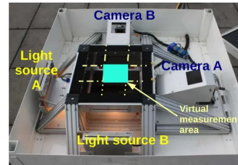
Figure 1. 2DVD measurement setup.

The manuscript is structured as follows. Section 2 de-scribes the experimental setup and the basic 2DVD data. tion 3 presents the hydrometeor classification model. Sec-tion 4 presents the main results and their quality assessment, while Sect. 5 provides examples of the outputs of the hy-drometeor classification. Section 6 concludes the paper and lists some future perspectives.

2 Data set description 2.1 Experiment locations

The 2DVD data employed in the experiments were collected during three distinct field campaigns, between Septem-ber 2009 and March 2013. The first campaign took place from September 2009 until June 2011 in Davos, Switzer-land: the 2DVD was deployed in the Swiss Alps, at an al-titude of about 2500 m a.s.l.Data for a total of 1700 h of pre-cipitation in liquid, mixed, and solid phase were collected during this time frame. The second campaign took place in Remoray, France, from December 2012 until March 2013, at an altitude of about 920 m, in the context of an exper-iment focused on melting hydrometeors. A total of 270 h of precipitation in solid, liquid, and mixed phase was col-lected in this experiment. The third complementary cam-paign includes about 200 h of data (mainly solid precipi-tation) collected by three 2DVD instruments between De-cember 2011 and March 2012 in the framework of the Global Precipitation Measurement mission (GPM, http:// pmm.nasa.gov/precipitation-measurement-missions), in the Cold-season Precipitation Experiment (GCPEx) that took place in Ontario, Canada.

2.2 2DVD instrument and data pre-processing

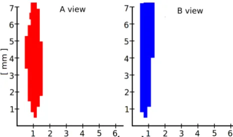
Figure 2. Example of A–B views of a non-realistic particle that

needs to be filtered.

most relevant features of the instrument. Figure 1 illustrates the 2DVD measurement principle (see Fig. 3 of Kruger and Krajewski, 2002, for more details).

Two orthogonal light sources coupled with two (A and B) line-scanning cameras generate two stacked measurement planes of about 11 cm×11 cm. The planes are vertically sep-arated by a distance of around 6.2–7 mm (the exact value is determined by mechanical calibration). The cameras capture the falling particles at a resolution of 512 pixels (0.2 mm) at 34 kHz, and the vertical distance between the measurement areas of cameras A and B enables the measurement of fall velocity.

The raw images need to be processed before being em-ployed. This involves the filtering of unreasonable measure-ments, as well as the rematching of the measurements taken from camera A and B in order to ensure that both images actually refer to the same particle. Filtering and rematching of 2DVD images is based on the work of Hanesch (1999) and Huang et al. (2010). We followed their methods, but with a noteworthy modification. Those studies, which were interested in snowfall only, restricted the maximum fall ve-locity to 4 and 6 m s−1, respectively. We increased this up-per boundary to 14 m s−1, large enough to include, with suf-ficient margins, the range of variation found in rain (e.g., Beard, 1976) and large graupel (List and Schemena, 1971).

Despite this filtering, some non-realistic particles can still be observed in the output. These particles appear as large ob-jects, vertically oriented and elongated, as shown in Fig. 2. Because of these peculiarities, they are easily identified and excluded from the analysis presented in this paper. The exact nature of these artifacts is unknown, but their vertical ori-entation and dimension suggest that they may be associated with small-scale wind effects, melting, or dripping, causing some particles to reside for an anomalous amount of time in the measurement areas of the two cameras. The proportion of rejected particles is on average 3 %, and it ranges between 0.5 and 13 % per day. A few precipitation events required higher rejection rates. They were excluded from the analysis presented in this work.

Table 1. List of descriptors chosen to describe the particles

recorded. Descriptors 1 and 2 come from the combination of camera A and B; 3 to 6 describe particle size, and 7 to 13 particle shape.

Symbol Full name Units 1 v Fall velocity [m s−1] 2 De Equivolumetric diameter [mm]

3 AA,B Shaded area [mm2]

4 PA,B Shaded perimeter [mm]

5 TA,B Particle thickness [mm]

6 WA,B Particle width [mm]

7 PF_A,B Pixel fraction [–] 8 FORMA,B Form index [–]

9 SqP_A,B Square pixel metric [–] 10 FDA,B Fractal dimension [–]

11 SI_A,B Shape index [–] 12 ELONGA,B Elongation [–]

13 ROUNDA,B Roundness [–]

Two additional potential sources of uncertainty (whose magnitude is currently not known in snowfall) are the im-age distortion that can occur when the horizontal component of the falling velocity of the particles is significant, and the local winds generated by the geometry of the instrument. To date, image distortion can only be corrected in rain, and in particular only for raindrops that possess an axis of rota-tional symmetry (Schönhuber et al., 2008). In contrast, the winds induced by the instrument itself can lead to an under-estimation of particles having lower density and dimension1. Further research, which is beyond the scope of this paper, is needed to develop correction schemes for snowfall measure-ments in order to compensate for these two potential issues. 2.3 From single particles to global features

Pairs of 2DVD A–B images are available for each parti-cle falling in the measurement area. For the purpose of the present work, it is useful to summarize this large amount of information by choosing a set of relevant descriptors2. Then, the statistical distributions of these descriptors in a time step

1t are used as input information for the hydrometeor clas-sification. The descriptors chosen in this work are listed in Table 1, and can be divided into three groups.

2.3.1 Joint descriptors

Two descriptors are obtained by combining the views of cam-eras A and B. They are particle falling velocityv[m s−1], and 1_{This issue is more severe for the first generation of the 2DVD}

instrument (Nespor et al., 2000). All the data employed in the present study were collected with second- and third-generation 2DVDs.

2_{The particle descriptors are calculated in the present work from}

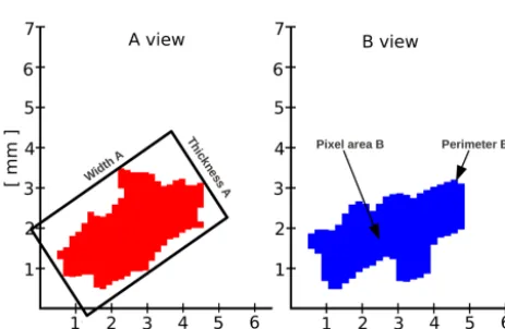
Figure 3. Examples of particles descriptors of 2DVD images

(cam-era A and B). On cam(cam-era A: width (WA [mm]) and thickness

(TA [mm]) of the bounding box enclosing the particle. On

cam-era B: particle apparent perimeter (PA[mm]) and shaded area (AA

[mm2]).

equivolumetric diameterDe[mm].Dedenotes the diameter of a sphere with the same volume as the falling particle.

This descriptor was originally developed for raindrops, for which volumes could be calculated accurately from the 2-D views. It can be extended to particles of any shape as a refer-ence measure of particle size. In the present work,Deis cal-culated according to the formulation of Huang et al. (2010). 2.3.2 Particle size

Other descriptors can be computed separately for camera A and camera B. Figure 3 illustrates some of them. The ap-parent shaded areas AA,B and perimeters PA,B are readily available from the 2DVD measurements, while thicknesses

TA,Band widthsWA,Bof each particle are defined with re-spect to a bounding box around the particle (Fig. 3).v,De, A,P,T, andWtogether describe the particle bulk dimension and velocity.

2.3.3 Particle shape

Additional descriptors are computed to better characterize particle shape. They are dimensionless shape metrics com-monly used in the analysis of land cover images for remote sensing (Jiao and Liu, 2012), adapted for use on 2DVD im-ages:

PFA,B= AA,B

Ar_A,B (0,1], (1)

FORMA,B= 4π AA,B

P_A2_,B (0,1

], (2)

SqP_A,B=1−4

p

AA,B PA,B

[1−2/ √

π ,1), (3)

FDA,B=2

ln(PA,B/4) ln(AA,B)

[1,2], (4)

SIA,B= PA,B

4pAA,B [

√

π /2,+∞], (5)

ELONGA,B= WA,B

TA,B

[1,+∞], (6)

ROUNDA,B=4 AA,B

π WA,B2

(0,1], (7)

whereAr_A,B[mm2] is the area of the bounding box calcu-lated for image A (or B). PFA,B is the pixel fraction and compares the shaded area with the area of the bounding box. PFA,Bis an index of compactness, as is the roundness index (ROUNDA,B), which compares the shaded area with a circular approximation. FORMA,Band square pixel metric SqP_A,Bare shape complexity indices based on the area-to-perimeter ratio (they increase with decreasing complexity), while fractal dimension FDA,Band shape index SIa,bare

in-dexes based on the perimeter-to-area ratio (they increase with increasing complexity). ELONGA,Bevaluates the degree of elongation of the particles.

As introduced above, the feature vector used in the SVM model refers to the distribution of descriptors in a time step

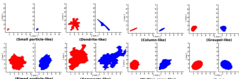
Figure 4. Examples of particle images (two camera views: A left, B right) belonging to time steps dominated by a particular hydrometeor

class.

3 Hydrometeor classification

This section details the proposed supervised classification approach. First we define the hydrometeor classes, then we detail how a training set is obtained, and finally we present the classifier employed and its implementation to the avail-able data set.

3.1 Hydrometeor classes and training set

The principle of supervised classification methods is to use a set ofNtrainlabeled observations (or a training set) to train a classifier that will learn how to interpret new unlabeled observations. In our case, we need to assign the appropri-ate dominant hydrometeor type to a selected population of time steps of length1t. The 2DVD offers the possibility to visualize the actual hydrometeor images, and the supervision was therefore conducted manually, according to the judge-ment of trained operators. Two operators independently in-terpreted the images by visualizing particle shapes, veloci-ties, and taking into account the on-site environmental con-ditions (time of the year, temperature). Additionally, for the data collected in Davos, X-band radar observations over the region were available (e.g., Schneebeli et al., 2013), thus pro-viding contextual information about the structure of the pre-cipitation and, in stratiform cases, about the altitude of the melting layer.

The visualization and pre-interpretation of a wide range of time steps led to the selection of eight hydrometeor classes to describe the possible precipitation types in the available data set. Figure 4 shows an example of a typical particle belong-ing to each class. The classes are small-particle-like (SP), dendrite-like (D), column-like (C), graupel-like (G), rimed-particle-like (RIM), aggregate-like (AG), melting-snow-like (MS), and rain (R). The “-like” is added to emphasize that this approach identifies the dominant type of hydrometeor, which does not necessarily imply that (i) there is only one type of hydrometeor in the considered time step and (ii) that all hydrometeors exhibit pristine shape and geometry.

The definitions for some hydrometeor classes require clar-ification. SP time steps refer to particles falling during ice-phase precipitation that, given their size and the resolution of the instrument (0.2 mm), do not allow for proper visual shape recognition. Small aggregates, as well as single ice crystals, can be assumed to belong to this class. RIM is observed when riming processes smooth the shapes of the hydrome-teors and increase their fall speed, while G time steps refer to fully developed graupel in which the original shape of the rimed crystal is no longer recognizable. MS is observed when the instrument records precipitation within the melting layer, and in these time steps raindrops, snowflakes, and smoother snowflakes with larger fall speed coexist in a mixed phase.

The creation of the training set involved the inspection of all the particles within each time step, in order to retrieve the dominant particle type and to provide the appropriate label. Particular attention was paid to select time steps that were as pure as possible, for the subsequent training of the classi-fier. The training set employed in the present work includes

Ntrain=400 time steps, each of them numerically character-ized by the 115 components of the associated feature vector xdefined in Sect. 2.3.

3.2 Classification method

In this section, we present the classifier used, the SVM. Then, we briefly detail an extension of the SVM that allows for the retrieval of the importance of each input feature (or group of features) in the model: SVM-MKL.

3.2.1 SVM

generalize well on a set of unknown samples for which we do not know the dominant hydrometeor typeXval= {xv}N_v=val1.

The SVM finds the best linear separation, of typef (x)= hw,xi +b, for which all training samples are at least at a dis-tance of 1 from the separating plane. In other words, for all training samples, f (x) must be greater or equal to 1. To differentiate between positive and negative examples, we also multiply this expression by 1 if the sample is of the positive class and by −1 if it is of the negative class (the two types of hydrometeors). To summarize, the constraint is

yi(hw,xii +b)≥1,∀i∈Ntrain. The strategy pursued by the SVM (more details in Boser et al., 1992) is to find the separa-tion which maximizes the distance between the closest points of each class, which are also called support vectors. This dis-tance is called the margin and is inversely proportional to the norm of the parameters vector, i.e.,||w||2. In order to allow for some classification errors, we also introduce a term xii,

which is non-zero for samples classified wrongly. The mar-gin maximization problem is the following one:

min

w,b,xi

₁

2||w|| 2

| {z }

Complexity of the function + C

Ntrain X

i=1 xii

| {z }

Training errors

(8)

with

(

yi[hx,wi +b]≥1−xii

xii≥0 and i=1, . . . , Ntrain.

Cis a parameter that controls the constraint of perfect clas-sification: if we allow some errors (by keeping C low), the margin becomes larger, thus reducing the dependence of the final model on training samples, which may be noisy or is-sued from errors in the measurements. A too high value ofC

drastically increases the value of the cost function as soon as errors are made. In this case, the resulting model will achieve perfect classification of the training samples, but the risk of over-fitting the training data and achieving poor generaliza-tion in the validageneraliza-tion phase is higher.

This optimization model is solved using Lagrangian mul-tipliersα, which allow us to rewrite the problem as

max

α

(_N

train X

i=1 αi−

1 2

Ntrain X

i,j=1

αiαjyiyjhxi,xji

)

(9)

s.t. 0≤αi ≤C and

Ntrain X

i=1

αiyi=0.

When the optimal solution of Eq. (9) is found (i.e., the vector of coefficientsα), the label of an unknown samplexv

is assigned on the basis of the sign of the decision function, i.e., its position with respect to the hyperplane (f (x)=0):

yv=sign Ntrain

X

i=1

αiyihxi,xvi +b

!

. (10)

In the present formulation, it can be observed that the SVM is only a binary classifier. A number of strategies exist

to reduce multiclass problems to binary problems, and in the present work the one-against-one rule was employed (Hastie and Tibshirani, 1998). The one-against-one rule builds as many binary classifiers as there are pairs of classes. Each classifier is therefore used to assign the time step to one of two possible classes. The time step is eventually classified into the class that received the most assignments.

3.2.2 Nonlinear SVM

The SVM, as has been discussed above, can only solve lin-ear problems (it defines a linlin-ear hyperplane). However, there is an elegant solution to solve nonlinear problems. Let us go back to Eqs. (9) and (10): the solution of the optimization does not depend on the training samples themselves but in-stead only on the dot products between samples (seehxi,xji

in Eq. 9). In the same way, the prediction for a new sample only depends on its dot products with the training samples (seehxi,xviin Eq. 10). Dot products are measures of

simi-larity between the samples. To perform nonlinear classifica-tion, we need to find an estimate of their similarity in a pro-jected space of higher dimensionH, where linear separation becomes possible3. To avoid explicitly defining the coordi-nates of the samples in the projected space, i.e.,φ (xi), we

can use functions that, even if expressed with points in the original space, correspond to dot products in the projected spaceH: these functions are called kernels. Without enter-ing mathematical details, which the interested reader can find in Scholkopf and Smola (2001), a kernel corresponds to a similarity function such thatK(xi,xj)= hφ(xi), φ(xj)i.

This means that, for a given projectionφ(·), the kernel com-puted fromxi andxj will correspond to their similarity in

the spaceHdefined byφ (·). A classification which is linear in the projected space is nonlinear in the original space, as illustrated in Fig. 5.

In practice, in order to obtain a nonlinear classification with the SVM, we replace the dot products in Eqs. (9) and (10) by kernel functions K(xi,xj)andK(xi,xv),

re-spectively. A classical kernel to obtain such a behavior is the radial basis function (RBF), which is computed as follows:

K(xi,xj)=exp

||xi−xj||2

2σ2

!

. (11)

The RBF kernel acts as a Gaussian similarity, which is max-imal when considering the same samples (K(xi,xi)=1),

and decreases jointly with the decrease of similarity between the samples. The bandwidthσ controls the steepness of the Gaussian bell.

3.2.3 SVM-MKL

Even if very successful, SVM remains a black-box model, in the sense that no information about the importance of the 3_{The Cover theorem states that the probability of linear}

(a)

x2

(b) (x1)2 2

2(x1x2)

(c) (d)

x1

(x2)

x2

x1 2

(x2)

(x1)2

2(x1x2)

Decision

func tion

Figure 5. Illustration of the nonlinear SVM. (a) A nonlinearly separable data set in the input spaceX, involving two classes (squares and circles). (b) Projection on a 3-D spaceHby the kernelK(xi,xj)= hxi,xji2. (c) Linear classification in the projected spaceH(filled dots

are support vectors). (d) Corresponding nonlinear decision function in the original spaceX. Adapted from Volpi et al. (2013).

initial variables can be retrieved from its results. All opera-tions are optimized in the projected spaceH: this means that, while it avoids computation of projection of the samples ex-plicitly, it also prevents the assessment of the importance of the different variables involved. Recent research has offered a solution to this problem by introducing the concept of mul-tiple kernel learning (MKL; Rakotomamonjy et al., 2008).

SVM-MKL builds on the so-called Mercer conditions, stating that a weighted sum of any positive definite func-tion (a requirement for all kernel funcfunc-tions) is again defi-nitely positive (Mercer, 1905). This means that we can de-sign a valid kernel by a linear combination ofMbase kernels

Km(xi,xj), each one considering single time step features

(in this caseM=115) or sets of time step features (in this caseM <115 and equals the number of groups of descrip-tors):

K(xi,xj)= M

X

m=1

dmKm(xi,xj). (12)

dmis the weight attributed to each kernelKmand is a mea-sure of the importance of this kernel in the combination, i.e., of the variables composing it. It usually sums up to 1. The SimpleMKL algorithm proposed in Rakotomamonjy et al. (2008) alternatively optimizes the weights and the SVM and at the same time retrieves the relative importance of each group (dm), and the SVM model associated with the final

weighted combination.

In our experiment, we used SimpleMKL to find the best combination of a series of RBF kernels Km, each one

as-signed to a set of features referring to the same particle de-scriptor (M=13; see Table 1). As an example,K1takes into account the eight statistical features (Q10, Q25, Q50, Q75, Q90, IQ75–25, IQ90–10, mean) associated with the hydrom-eteor fall velocityvdescriptor,K2the eight features associ-ated with the equivolumetric diameterDe, and so on.

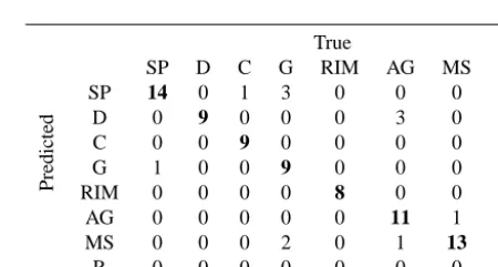
Table 2. Example of a confusion matrix obtained during validation

of the SVM classification for a validation setN_val∗ of 100 observa-tions. Correct classifications are situated on the diagonal, and mis-classifications are in the off-diagonal entries.

True

Predicted

SP D C G RIM AG MS R SP 14 0 1 3 0 0 0 0 D 0 9 0 0 0 3 0 0 C 0 0 9 0 0 0 0 0 G 1 0 0 9 0 0 0 0 RIM 0 0 0 0 8 0 0 0 AG 0 0 0 0 0 11 1 0 MS 0 0 0 2 0 1 13 0 R 0 0 0 0 0 0 0 15

4 Results and discussion

4.1 Performance assessment metrics

The evaluation of the accuracy of classification is conducted via different metrics. The availableNtrain training observa-tions are divided into two parts (N_train∗ andN_val∗ ).N_train∗ ob-servations are used as a training set to optimize the SVM parametersCandσ and to train the SVM, while the remain-ingN_val∗ observations are kept for validation. A comparison is made between the SVM classification output{y_i∗}N

∗

val

i=1, and the true labels{yi}

N_val∗

i=1 by evaluating an 8×8 confusion ma-trix C, as shown in Table 2. The elements C(i, j )contain the number of observations classified in theith class, which in reality belong to thejth class. The diagonal contains the correct classifications.

Given the confusion matrix, the global performance of the classifier is quantified by the overall accuracy (OA), and Co-hen’s kappa (K):

OA= S

P

i=1 C(i, i)

N ×100, (13)

K=OA−Pest 1−Pest

Pest= S

P

i=1 S

X

j=1 Cj,i

S

X

j=1 Ci,j

!

N2 ,

whereSis the total number of classes, andN the total num-ber of observations (in our case S=8 and N=N_val∗ ). K

takes into account the correct prediction that might occur by chance, namelyPest, and is a robust metric in the case of un-balanced classes.

Then, we look at the performances obtained within each class. For this purpose, we use

OAk=

C(k, k) S

P

i=1 C(k, i)

×100, (15)

PODk=

C(k, k) S

P

i=1 C(i, k)

, (16)

POFDk=

S

P

i=1 C(k, i)

−C(k, k)

S

P

i=1 C(k, i)

, (17)

where OAk is the accuracy of the kth class, and PODk and

POFDkare respectively the associated probabilities of

detec-tion and false detecdetec-tion.

4.2 Evaluation of the quality of the training set

Ntrainobservations are available in total as a training set, and we must verify that this amount is sufficient for the present task. In other words, we want to assess here whether a larger

Ntrain would significantly improve the hydrometeor classi-fication. To do so we proceeded as follows: (1)Ntrain=400 was initially randomly split intoN_train∗ =300 andN_val∗ =100; (2) N_train∗ was iteratively reduced in size, while the original

N_val∗ was kept for validation; (3) evaluation of the perfor-mance was conducted at each step; and (4) steps (1)–(3) were repeated with 200 realizations of the original split.

Figure 6 shows the evolution of K as a function of the number of training samples in the training set (N_train∗ ). We can observe thatN_train∗ larger than 200 did not lead to significant improvements in terms ofK, while whenN_train∗ was smaller than 100, the performances started to degrade sharply. These results suggest that the total available labeled samples (400) are sufficient for the present classification task.

4.3 Evaluation of the classification performances For validation purposes, we now focus on 200 realiza-tions of the caseN_train∗ =300,N_val∗ =100. The classification achieved accurate global results, both in terms of OA and

K. As shown in Table 3,Kand OA mean values were 0.88 and 89 %, and in 90 % of the cases they took values higher

Figure 6. Evolution ofK[–] as a function of the training set size. The solid red line indicates the median, while the blue and brown areas represent Q75–25 and Q90–10, respectively. The size of the training set was varied with a step of 1 between 300 and 20. Statis-tics are based on 200 realizations.

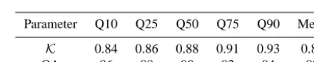
Table 3. Mean values and relevant quantiles ofK[–] and OA [%] calculated over 200 iterations of the SVM validation procedure.

Parameter Q10 Q25 Q50 Q75 Q90 Mean

K 0.84 0.86 0.88 0.91 0.93 0.88

OA 86 88 90 92 94 89

than 0.84 and 86 %, respectively. Additionally,K tended to be close to OA, indicating that correct classification occur-ring by chance is very unlikely.

The classification performance associated with each hy-drometeor class is summarized in Fig. 7. It can be observed that all the hydrometeor classes were identified with median OAkalways greater than 84 %, PODkgreater than 0.84, and

POFDk lower than 0.16. Overall, rainfall (R) hydrometeor

class achieved the best scores, together with columns (C). R hydrometeors showed a PODkequal to 1, meaning that errors

for this class were uniquely false detection. In contrast, C hy-drometeors showed low POFDkand OAkvery close to 1, and

the errors for this class were due mainly to missed detections, with PODkwith median scores around 0.9. Graupel (G) was

mostly affected by missed detections, and showed a relatively large interquantile spread for PODk, around the median value

of 0.87. Small particles (SP) had the highest false detection rate, with median POFDk close to 0.15. Dendritic snow (D)

exhibited the largest interquantile spreads, around otherwise satisfactory median values of 87 % (OAk), 0.87 (PODk), and

0.13 (POFDk), followed by rimed particles (RIM) that

Figure 7. Bar plots of (a) OAk[%], (b) PODk[–], (c) POFDk

asso-ciated with the eight hydrometeor classes undergoing classification. Statistics were calculated over 200 realizations of the SVM valida-tion.

correctly predicted, with lower interquantile spread, median OAk larger than 88 %, PODk larger than 0.88, and POFDk

lower than 0.12.

A last consideration concerns the choice of SVM as a clas-sifier. Other methods are used to solve similar tasks in var-ious fields of the environmental sciences, for example lin-ear discriminant analysis (LDA) or neural networks (NN) (e.g., Goosaert and Alam, 2009; Robert et al., 2013). Com-parison with these two methods showed that the proposed SVM scheme outperforms LDA by more than 25% and NN by more than 15% in terms ofK.

4.4 Ranking of descriptors

The SimpleMKL algorithm was applied to learn the most rel-evant descriptors in the classification process, as explained in Sect. 3.2.3. Referring to Eq. (12), it was observed that 5 groups of features out of the 13 (1 per descriptor, each in-cluding the 8 or 9 statistical features extracted from its dis-tribution in1t=60 s) accounted for about 70 % (Fig. 8) of the total weights and therefore are considered hereafter as the most important ones. They are, in decreasing order of importance, pixel fraction PF, velocityv, equivolume diam-eter De, form index FORM, and thicknessT, with associ-ated weights dm of 0.193, 0.181, 0.13, 0.112, and 0.098,

respectively. This does not imply that the remaining eight

Figure 8. Weightsdmof the 13Kmkernels, associated with the 13

particle descriptors used in the present study.

descriptors were negligible in the classification process, but that we expect to find a more immediate and intuitive physi-cal meaning in these five top-ranked ones.

5 Application on unlabeled data

This section presents some examples of the classification out-put, on data not included in the training set of the algorithm, and collected during the measurement campaign in Davos. 5.1 17 March 2011

A snowfall event occurring on 17 March 2011 is presented in Fig. 9. The air temperature recorded in the very close vicinity (less than 50 m away) was constantly below freezing (≈ −5◦C) through the entire event duration, and different ice-phase hydrometeors were identified in the time window shown here. Initially (07:00–09:00 UTC) precipitation was dominated by small particles (SP), followed by a phase of instability (09:00–10:00 UTC) characterized by sharp varia-tions in the identified hydrometeor classes. During the next relatively stable phase (10:00–12:30 UTC), graupel (G) and larger rimed particles (RIM) were identified. Panels (b), (c), and (d) of Fig. 9 illustrate the behavior in time of the three top-ranked particle descriptors, namely pixel fraction PF, equivolume diameterDe, and fall velocityv. The median PF was around 0.7 during the entire event, indicating relatively high particle compactness. The medianDewas initially be-low 1 mm (SP phase), and it increased to values between 1 and 2 mm in the latter part of the event characterized mostly by G and RIM classes.v exhibited the same trends as De, and it increased when rimed particles and graupel were dom-inant.

5.2 12 January 2011

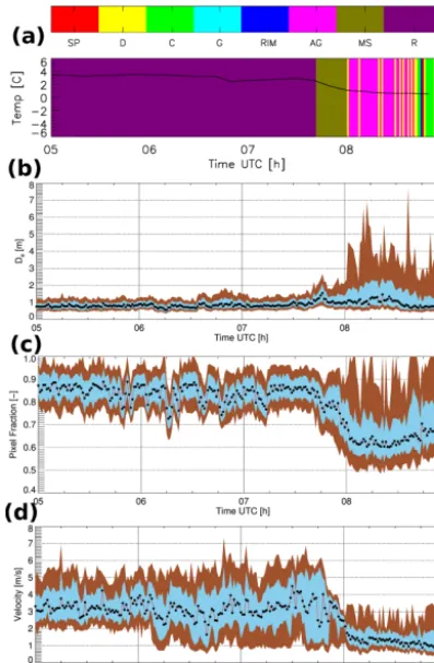
Figure 9. Snowfall event recorded on 17 March 2011. Time series

of (a) dominant hydrometeor type as classified with the SVM and local ambient temperature [◦C], as measured by a closely located (distance≤50 m) weather station; (b)De[mm]; (c) pixel fraction

of camera A PFA; and (d) fall velocityv[m s−1]. In panels (b), (c), and (d), black dots connected by the red solid line indicate the

median value, while the shaded areas depict Q90–Q10 and Q75– Q25, respectively.

8 mm (AG). Particle compactness was lower, with median PF below 0.7 throughout the event, and slightly lower for D than for AG. This is due to the higher geometrical complex-ity of aggregates and dendrites relative to small particles and graupel. The velocityvdid not exhibit peculiar trends, and it remained around values of 1 m s−1in median.

5.3 5 August 2010

The precipitation event that occurred on 5 August 2010 (Fig. 11) illustrates the transition between liquid-phase and ice-phase precipitation well. In the first part of the event (05:00–07:45 UTC) air temperature was around 4◦_{C, and} it dropped to 0◦C in the second part of the event (07:45– 08:00 UTC). After 08:00 UTC the air temperature stabilized again around 0◦C. These trends in temperature are directly reflected in the dominant hydrometeor types classified: ini-tially rain (R), then melting snow (MS), and finally aggre-gates (AG). The rain was characterized by small De and 2≤v≤5 m s−1 (i.e., light rain), which is larger than the

Figure 10. As in Fig. 9 but for 12 January 2011.

typical velocities of ice-phase hydrometeors, and very high compactness, with a median PF around 0.9. In the transition from R to MS and AG, a clear and relatively smooth trend was observed for the three descriptors shown:vdecreased to median values around 1 m s−1_{; the spread ofD}

e increased; and the median PF dropped to 0.6 in the AG phase at the same time, as the geometrical complexity of falling hydrom-eteors increased.

Generally, the transition between R, MS, and AG was well captured in the large available data set. Figure 12 shows the relative number of classifications for each of these three types of hydrometeors as a function of the temperature. Please note that temperature has not been used as an input in the pro-posed system (Table 1). R always occurred at positive tem-peratures, MS maximum occurrence was between 2 and 1◦C, and AG around 0 and−1◦C (in agreement with Hobbs et al., 1974). These results give us confidence in the ability of the proposed technique to provide a meaningful classification.

6 Summary and conclusions

Figure 11. As in Fig. 9 but for 5 August 2010.

time steps with length1t=60 s. The SVM was trained with 400 examples labeled by expert users, and outputs the dom-inant hydrometeor type within1t. Additionally, an estima-tion of the relative descriptive importance of the input fea-tures is provided, which is of particular interest when higher-level information on the particle characteristics is required.

Discrimination is performed between eight hydrome-teor classes: small-particle-like, dendrite-like, column-like, graupel-like, rimed-particle-like, aggregate-like, melting-snow-like, and rain. Evaluation of the classification perfor-mance was conducted both in global and class-specific terms. The classifier achieved accurate results, with median OA and

K of 90 % and 0.88, respectively. Each of the classes were identified with a median accuracy exceeding 84 %.

Additionally, once trained, the classifier is fast enough to be potentially implemented in real time.

Three classification examples together with the time evo-lution of the top-ranked particle descriptors were used to illustrate the typical classification products in pure snow-fall events and in the transition between snowsnow-fall and rain-fall. Global hydrometeor-type behavior as well as small-scale fluctuations could be observed.

Figure 12. Distributions of the occurrence of AG, MS, and R as a

function of air temperature. The distributions are obtained by aggre-gation of all the 2DVD measurements collected during the field ex-periments in Davos 2009–2011 and Remoray 2012–2013, and tem-perature data are given by closely located weather stations.

The proposed classification of hydrometeors from the 2DVD measurements provides additional information that can help to better understand the microphysical processes characterizing ice-phase precipitation events. This work has the potential to be a starting point for ground-based quantita-tive evaluation of products derived from polarimetric weather radars. It can also be adapted and implemented to receive inputs from other particle imaging systems (one or two di-mensional), either ground-based or airborne, provided that human interpretation can be carried out for the particle in the training set and that geometrical descriptors can be computed from the particle images.

Appendix A: Minimum number of particles for a reliable classification

The proposed classification method employs a set of sta-tistical features calculated overN particles as input, within a time step of length1t. Thus, when N is small, sampling problems can affect the estimation of such statistics. We want to set a minimumNmin, such that ifN > Nmin, the classifica-tion output is reliable.

Figure A1a shows the contribution that time steps of length

1t with smallNhad with respect to the total amount of data available, both in terms of total number of particles and in terms of total number of time steps.

We can observe that time steps with lowNcontribute neg-ligibly to the total particle count, but significantly to the total count of available time steps. In other words, time steps with a low number of particles carry only a small part of the total precipitation, but they are observed frequently.

Figure A1b illustrates the classification performance achieved whenN <60. This was obtained by taking random subsets of the available training set (with known labels) and using them as validation of the SVM algorithm trained previ-ously. We can observe that the performance degraded sharply forN <20, and becomes more than 20 % lower than in cases withN >60. A thresholdNmin=20 was therefore selected.

Acknowledgements. For the data from Switzerland, we thankfully

acknowledge the help of Nick Dawes, as well as many others at the WSL Institute for Snow and Avalanche Research SLF.

The participation of Devis Tuia was financed through the Swiss National Science (SNF), project number PZ00P2_136827.

For the data from Canada, we are thankful to Patrick Gatlin, Walt Petersen, Gwo-Jong Huang, and David Hudak.

We finally thank Carine Berne for accepting various instruments in her garden for an entire winter.

Edited by: F. S. Marzano

References

Beard, K. V.: Terminal velocity and shape of cloud and precipitation drops aloft, J. Atmos. Sci., 33, 851–864, 1976.

Boser, B., Guyon, I., and Vapnik, V.: A training algorithm for opti-mal margin classifiers, in: 5th ACM Workshop on Computational Learning Theory, 144–152, Pittsburgh, USA, 1992.

Brandes, E. A., Ikeda, K., Zhang, G., Schonhuber, M., and Rasmussen, R. M.: A statistical and physical description of hydrometeor distributions in Colorado snowstorms using a video disdrometer, J. Appl. Meteor. Clim., 46, 634–650, doi:10.1175/JAM2489.1, 2007.

Camps-Valls, G. and Bruzzone, L.: Kernel-based methods for hy-perspectral image classification, IEEE T. Geosci. Remote Sens., 43, 1351–1362, doi:10.1109/TGRS.2005.846154, 2005. Camps-Valls, G. and Bruzzone, L. (Eds.): Kernel Methods for

Re-mote Sensing Data Analysis, Wiley, 2009.

Cao, Q., Zhang, G. F., Brandes, E., Schuur, T., Ryzhkov, A., and Ikeda, K.: Analysis of video disdrometer and polarimetric radar data to characterize rain microphysics in Oklahoma, J. Appl. Meteor. Clim., 47, 2238–2255, doi:10.1175/2008JAMC1732.1, 2008.

Chandrasekar, V., Keranen, R., Lim, S., and Moisseev, D.: Re-cent advances in classification of observations from dual polarization weather radars, Atmos. Res., 119, 97–111, doi:10.1016/j.atmosres.2011.08.014, 2013.

Cover, T. M.: Geometrical and statistical properties of systems of linear inequalities with applications in pattern recognition, IEEE Transactions on Electronics and Computers, EC-14, 326–334, 1965.

Delanoe, J., Protat, A., Jourdan, O., Pelon, J., Papazzoni, M., Dupuy, R., Gayet, J. F., and Jouan, C.: Comparison of air-borne in situ, airair-borne radar-lidar, and spaceair-borne radar-lidar retrievals of polar ice cloud properties sampled during the PO-LARCAT campaign, J. Atmos. Oceanic Technol., 30, 57–73, doi:10.1175/JTECH-D-11-00200.1, 2013.

Dolan, B. and Rutledge, S. A.: A theory-based hydrom-eteor identification algorithm for X-band polarimet-ric radars, J. Atmos. Oceanic Technol., 26, 2071–2088, doi:10.1175/2009JTECHA1208.1, 2009.

Elmore, K. L.: The NSSL hydrometeor classification algorithm in winter surface precipitation: evaluation and future develop-ment, Weather Forecast., 26, 756–765, doi:10.1175/WAF-D-10-05011.1, 2010.

Feind, R. E.: Comparison of three classification methodologies for 2D probe hydrometeor images obtained from the armored T-28 aircraft, Tech. Rep. SDSMT/IAS/R08-01, Institute of

Atmo-spheric Sciences, South Dakota School of Mines and Technol-ogy, Rapid City, SD, USA, 2008.

Foresti, L., Tuia, D., Kanevski, M., and Pozdnoukhov, A.: Learning wind fields with multiple kernels, Stoch. Env. Res. Risk A., 25, 51–66, doi:10.1007/s00477-010-0405-0, 2011.

Goosaert, E. and Alam, R.: Ensemble classifier for winter storm precipitation in polarimetric radar data, in: Seventh conference on artificial intelligence and its applications to the environmental sciences, Phoenix, USA, 2009.

Hanesch, M.: Fall velocity and shape of snowflakes, Ph.D. thesis, Swiss Federal Institute of Technology Zurich, 1999.

Hastie, T. and Tibshirani, R.: Classification by pairwise coupling, Ann. Stat., 26, 451–471, 1998.

Hobbs, P. V., Chang, S., and Locatelli, J. D.: The dimensions and aggregation of ice crystals in natural clouds, J. Geophys. Res., 79, 2199–2206, doi:10.1029/JC079i015p02199, 1974.

Houze, R. A. J.: Cloud dynamics, Academic Press, San Diego, 1993.

Huang, G., Bringi, V. N., Cifelli, R., Hudak, D., and Petersen, W. A.: A methodology to derive radar reflectivity liquid equivalent snow rate relations using C-band radar and a 2D video disdrometer, J. Atmos. Oceanic Technol., 27, 637–651, 2010.

Jiao, L. and Liu, Y.: Analyzing the shape characteristics of land use classes in remote sensing imagery, ISPRS Annals of Pho-togrammetry, Remote Sens. Spatial Inf. Sci., I-7, 135–140, doi:10.5194/isprsannals-I-7-135-2012, 2012.

Kruger, A. and Krajewski, W. F.: Two-dimensional video disdrom-eter: a description, J. Atmos. Oceanic Technol., 19, 602–617, 2002.

List, R. and Schemena, R.: Free-fall behavior of planar snow crys-tals, conical graupel and small hail, J. Atmos. Sci., 28, 110–115, doi:10.1175/1520-0469(1971)028<0110:FFBOPS>2.0.CO;2, 1971.

Löffler-Mang, M. and Joss, J.: An optical disdrometer for measuring size and velocity of hydrometeors, J. Atmos. Oceanic Technol., 17, 130–139, 2000.

Marzano, F. S., Cimini, D., and Montopoli, M.: Investigating precipitation microphysics using ground-based microwave re-mote sensors and disdrometer data, Atmos. Res., 97, 583–600, doi:10.1016/j.atmosres.2010.03.019, 2010.

Mercer, J.: Functions of positive and negative type and their con-nection with the theory of integral equations, Philos. Tr. R. Soc., CCIX, 215–228, 1905.

Nespor, V., Krajewski, W. F., and Kruger, A.: Wind-induced error of raindrop distribution measurement using a two-dimensional video disdrometer, J. Atmos. Oceanic Technol., 17, 1483–1492, 2000.

Rakotomamonjy, A., Bach, F., Canu, S., and Grandvalet, Y.: Sim-pleMKL, J. Mach. Learn. Res., 9, 2491–2521, 2008.

Robert, S., Foresti, L., and Kanevski, M.: Spatial prediction of monthly wind speeds in complex terrain with adaptive general regression neural networks, Int. J. Climatol., 33, 1793–1804, doi:10.1002/joc.3550, 2013.

Scholkopf, B. and Smola, A. J.: Learning with Kernels: Support Vector Machines, Regularization, Optimization, and Beyond, MIT Press, Cambridge, MA, USA, 2001.

Schönhuber, M., Lammer, G., and Randeu, W. L.: The 2D video dis-drometer, Chapter 1 in: Precipitation: Advances in Measurement, Estimation and Prediction, edited by: Michaelides, S., 2008. Schuur, T. J., Ryzhkov, A. V., Zrnic, D. S., and

Schon-huber, M.: Drop size distributions measured by a 2D video disdrometer: Comparison with dual-polarization radar data, J. Appl. Meteor., 40, 1019–1034, doi:10.1175/1520-0450(2001)040<1019:DSDMBA>2.0.CO;2, 2001.

Shupe, M. D.: A ground-based multisensor cloud phase classifier, Geophys. Res. Lett., 34, L22809, doi:10.1029/2007GL031008, 2007.

Straka, J. M., Zrnic, D. S., and Ryzhkov, A. V.: Bulk hydrometeor classification and quantification using polarimetric radar data: synthesis of relations, J. Appl. Meteor., 39, 1341–1372, 2000. Sullivan, S.: Evaluation of support vector machines and minimax

probability machines for weather prediction, in: Seventh confer-ence on artificial intelligconfer-ence and its applications to the environ-mental sciences, Phoenix, USA, 2009.

Thurai, M. and Bringi, V. N.: Drop axis ratios from a 2D video disdrometer, J. Atmos. Oceanic Technol., 22, 966–978, doi:10.1175/JTECH1767.1, 2005.

Thurai, M., Hudak, D., and Bringi, V. N.: On the possible use of copolar correlation coefficient for improving the drop size dis-tribution estimates at C band, J. Atmos. Oceanic Technol., 25, 1873–1880, doi:10.1175/2008JTECHA1077.1, 2008.

Thurai, M., Szakall, M., Bringi, V. N., Beard, K. V., Mitra, S. K., and Borrmann, S.: Drop shapes and axis ratio distributions: comparison between 2D video disdrometer and wind-tunnel measurements, J. Atmos. Oceanic Technol., 26, 1427–1432, doi:10.1175/2009JTECHA1244.1, 2009.

Tuia, D., Camps-Valls, G., Matasci, G., and Kanevski, M.: Learning relevant image features with multiple-kernel clas-sification, IEEE T. Geosci. Remote Sens., 48, 3780–3791, doi:10.1109/TGRS.2010.2049496, 2010.

Volpi, M., Tuia, D., Bovolo, F., Kanevski, M., and Bruzzone, L.: Supervised change detection in VHR images using contextual information and support vector machines, Int. J. Appl. Earth Obs. Geoinf., 20, 77–85, doi:10.1016/j.jag.2011.10.013, 2013. Xue, M., Droegemeier, K. K., and Wong, V.: The Advanced

Re-gional Prediction System (ARPS); A multi-scale nonhydrostatic atmospheric simulation and prediction model. Part I: model dy-namics and verification, Meteorol. Atmos. Phys., 75, 161–193, doi:10.1007/s007030070003, 2000.

Yuter, S. E., Kingsmill, D. E., Nance, L. B., and Loeffler-Mang, M.: Observations of precipitation size and fall speed characteristics within coexisting rain and wet snow, J. Appl. Meteor. Clim., 45, 1450–1464, doi:10.1175/JAM2406.1, 2006.

Zeng, J. and Qiao, W.: Support vector machine-based short-term wind power forecasting, in: Power Systems Con-ference and Exposition (PSCE), 2011 IEEE/PES, 1–8, doi:10.1109/PSCE.2011.5772573, 2011.

Zhang, G., Xue, M., Cao, Q., and Dawson, D.: Diagnosing the in-tercept parameter for exponential raindrop size distribution based on video disdrometer observations: model development, J. Appl. Meteor. Clim., 47, 2983–2992, doi:10.1175/2008JAMC1876.1, 2008.