www.atmos-meas-tech.net/7/3685/2014/ doi:10.5194/amt-7-3685-2014
© Author(s) 2014. CC Attribution 3.0 License.
Mixing-layer height retrieval with ceilometer and Doppler lidar:
from case studies to long-term assessment
J. H. Schween1, A. Hirsikko2, U. Löhnert1, and S. Crewell1
1Inst. f. Geophysics and Meteorology, Univ. of Cologne, Cologne, Germany 2Forschungszentrum Jülich GmbH, Institut für Energie-und Klimaforschung:
Troposphäre (IEK-8), Jülich, Germany
Correspondence to: J. H. Schween ([email protected])
Received: 14 February 2014 – Published in Atmos. Meas. Tech. Discuss.: 30 April 2014 Revised: 18 September 2014 – Accepted: 24 September 2014 – Published: 8 November 2014
Abstract. Aerosol signatures observed by ceilometers are frequently used to derive mixing-layer height (MLH) which is an essential variable for air quality modelling. However, Doppler wind lidar measurements of vertical velocity can provide a more direct estimation of MLH via simple thresh-olding. A case study reveals difficulties in the aerosol-based MLH retrieval during transition times when the mixing layer builds up in the morning and when turbulence decays in the afternoon. The difficulties can be explained by the fact that the aerosol distribution is related to the history of the mixing process and aerosol characteristics are modified by humidifi-cation. The results of the case study are generalized by eval-uating one year of joint measurements by a Vaisala CT25K and a HALO Photonics Streamline wind lidar. On average the aerosol-based retrieval gives higher MLH than the wind lidar with an overestimation of MLH by about 300 m (600 m) in the morning (late afternoon). Also, the daily aerosol-based maximum MLH is larger and occurs later during the day and the average morning growth rates are smaller than those de-rived from the vertical wind. In fair weather conditions clas-sified by less than 4 octa cloud cover the mean diurnal cycle of cloud base height corresponds well to the mixing-layer height showing potential for a simplified MLH estimation.
1 Introduction
The atmospheric boundary layer (ABL) is the lowest part of the atmosphere that is in contact with the Earth’s sur-face (American Meteorological Society, 2013). The mixing layer is a type of ABL where exchange processes between the
Earth’s surface and the atmosphere occur via turbulent mix-ing (see e.g. Oke, 1987; American Meteorological Society, 2013). Gaseous and particulate constituents emitted from the surface become well mixed within the ML which is capped by a temperature inversion or statically stable layer of air. Therefore, aerosol particle concentration is high in the mix-ing layer whereas further up in the free troposphere aerosol concentrations are generally much lower. Atmospheric pol-lutants are dispersed within the ML, and thus mixing-layer height (MLH) is an important parameter for air quality ap-plications. Any model that attempts to predict concentrations needs MLH as a parameter or must be able to describe its evolution (e.g. Collier et al., 2005; White et al., 2009). Fur-thermore, in a convective boundary layer, cumulus clouds can only develop if the MLH reaches the convective conden-sation level, making it thus a relevant quantity for numerical weather prediction.
convection decays and a neutral or slightly stable layer forms, called the residual layer (RL). At night the emission of long-wave radiation by the surface leads to strong cooling and the formation of a stable nocturnal boundary layer (NBL) close to the surface and below the RL. In low wind speed situa-tions stratification of the NBL can be very strong, leading to a decoupling of the layer above and as a consequence to the formation of the so-called nocturnal low-level jet
(Garratt, 1994), which may induce intermittent turbulent mixing (Banta et al., 2006). In the case of moderate surface winds during night a shallow nocturnal mixing layer may be induced by surface roughness and stored heat especially in urban areas (Souch and Grimmond, 2006). Strong winds are usually connected to strong shear especially close to the sur-face and thus also induce turbulent mixing which can reach even during night heights similar to those of a convective ML.
A number of methods exist to determine the MLH from different measurements (Seibert et al., 2000). Most of them are based on proxies for the mixing process, such as temper-ature, humidity or Richardson number. These parameters are frequently used in radiosonde-based retrievals, which are of-ten considered to be the most reliable as they are based on in situ measured parameters, and are therefore used as reference in several studies (e.g. Eresmaa et al., 2006; Sicard et al., 2006; Münkel et al., 2007; O’Connor et al., 2010). However, determination of the MLH from radiosonde data is not that straightforward because no unambiguous separation between ML and the atmosphere above might be found (Seibert et al., 2000). Additionally, radiosondes measure properties along their flight path and their data might not be representative for the atmospheric column above the measurement site. Due to the fact that a radiosonde follows the horizontal wind during its ascent, it tends to move into regions with convergence and avoids regions with divergence. As a result radiosonde pro-files are biased towards properties of rising plumes in convec-tive situations. In addition, a major shortcoming of radioson-des for MLH estimation is their coarse temporal resolution.
Many of the radiosonde drawbacks can be overcome by continuously operating ground-based remote sensing in-struments. Lidar (Light Detection and Ranging) systems have been used for atmospheric research since the 1960s (Weitkamp, 2005). An aerosol lidar determines the aerosol backscatter coefficientβwhich depends on number concen-tration, size and optical properties of the aerosol particles. Assuming that the main source for aerosol and its precur-sors is at the surface, turbulent mixing will lead to a uniform high aerosol concentration in the ML and a distinct gradi-ent to much lower concgradi-entrations in the atmosphere above. Thus it should be possible to derive MLH from lidar by us-ing the aerosol backscatter as a proxy. A number of different lidar-based algorithms exist to detect MLH (see e.g. Emeis et al., 2008). They are based on evaluating the gradient of the backscatter profile (Endlich et al., 1979), its logarithm (i.e. the relative gradient) (Senff et al., 1996), fitting to a function
(Steyn et al., 1999; Eresmaa et al., 2012), application of the Haar wavelet analysis (Davis et al., 2000; Brooks, 2003; Haij et al., 2006), or a threshold for the backscatter (e.g. Harvey et al., 2013). Even though advantages and disadvantages of different methods have been investigated by several studies (see e.g. Sicard et al., 2006; Haij et al., 2007; Eresmaa et al., 2012; Haeffelin et al., 2012), no consensus on a specific al-gorithm has been reached yet.
Lidar ceilometers are robust power, cost and low-maintenance lidars designed to determine the cloud base height (ceiling) but also provide the backscatter profile, though with less sensitivity than a lidar. Several studies have proposed that ceilometer-measured backscatter profiles can be used to derive the MLH (e.g. Münkel et al., 2007; Eresmaa et al., 2006, 2012). Many airports, weather services, research institutions etc. operate ceilometers (see http://www.dwd.de/ ceilomap), and therefore, attempts are made to use them as a network for aerosol retrieval (e.g. Wiegner et al., 2014) but also of MLH observations (e.g. Haij et al., 2007; Haeffelin et al., 2012).
Doppler lidars offer a direct approach to investigate the ABL mixing (e.g. Cohn and Angevine, 2000; Hogan et al., 2009). Instead of measuring a proxy for the vertical mixing, Doppler lidars can measure directly the vertical air veloc-ity. Engineering progress but also growth of the wind en-ergy industry in the last two decades have led to the de-velopment of affordable and robust Doppler lidar systems (e.g. Pearson et al., 2010). MLH can be estimated by us-ing a threshold value for the vertical velocity standard devia-tionσw(e.g Tucker et al., 2009; Pearson et al., 2010; Barlow
et al., 2011; Träumner et al., 2011). Another method is to use turbulent energy dissipation rate as proposed by O’Connor et al. (2010). This method is based on the assumption that measurements take place in the inertial subrange. However, the effort to ensure this is rather high (investigation of tur-bulent spectra) and reduces the universality of the method. Martucci et al. (2012) identify the MLH as the level of a dis-tinct negative gradient in theσw profile. This is somehow a
contradiction to the semi-theoretical profiles which show a smooth decay with more or less constant gradients towards the top of the ML (Lenschow et al., 1980; Sorbjan, 1989). In their multi-sensor approach for a boundary layer classifi-cation Harvey et al. (2013) use the second derivative of the vertical velocity variance with respect to height: if the profile is convex in the lower half of the ABL it is a ML with mixing originating from the surface. Träumner et al. (2011) discuss several methods based on the semi-theoreticalσw profile as
proposed by Lenschow et al. (1980). They find that the use of a threshold forσwis the most robust method.
height of the layer within which the largest vertical wind speeds occur. Tucker et al. (2009) test different retrievals based on vertical velocity variance, horizontal wind shear and lidar backscatter from a ship-based Doppler lidar dur-ing a 44-day campaign in the Gulf of Mexico. A compari-son of 99 selected best MLHs derived from different meth-ods and radiosondes gives a correlation of 0.87. During a 10-week campaign in a tropical rainforest Pearson et al. (2010) find significantly lower MLH derived from aerosol backscat-ter than those retrieved from wind lidar, which they attribute to aerosol particle growth within humid layers, gradients in the residual layer, and clouds. A 1-month campaign in Lon-don, UK, described by Barlow et al. (2011) shows good agreement between aerosol- and vertical wind based MLH during night but reveals a systematic underestimation of the aerosol-based MLH during daytime. Träumner et al. (2011) investigate 12 days of data from different campaigns in cen-tral Europe. A Doppler wind lidar is used to derive MLH from aerosol backscatter and vertical wind speed. Compari-son of both retrievals shows a high correlation (R= 0.91) but also large scatter with individual differences in the order of 500 m, which are attributed to the fact that the turbulence-based height gives the current extent of the ML whereas the aerosol-based height gives a measure of past MLH.
In general, studies agree that MLH is only reliably re-trieved from aerosol backscatter during noon hours when the convective boundary layer is fully developed and topped by the clean, free troposphere (e.g. Eresmaa et al., 2012; Träum-ner et al., 2011) Nevertheless, some recent studies investi-gated the climatology of e.g. the maximum MLH or the ML growth rate (e.g. Baars et al., 2008; Cimini et al., 2013; Ko-rhonen et al., 2014) not taking into account any limitations of the MLH retrieval during certain conditions. Especially, eval-uating the growth rate between some hours after sunrise and maximum MLH assumes that there are no limitations of the MLH retrieval during this time. Therefore a quantification of the errors of aerosol-based MLH retrievals is necessary. MLH retrieval based on Doppler wind lidar gives the oppor-tunity to evaluate this on high temporal resolution and over a long time period, if an automated system is used.
The aim of this work is to estimate and compare MLH de-rived from stand-alone ceilometer aerosol particle backscat-ter profiles and from Doppler lidar vertical velocity standard deviation profiles based on 1 year of continuous observa-tions. The vertical wind speed based MLH retrieval may be seen as a reference as it is based on the variable that causes the vertical mixing, whereas aerosol-based retrievals use the aerosol backscatter as a proxy. In this way, the potential per-formance of a low-cost ceilometer network for MLH estima-tion can be assessed.
2 Instruments and retrievals
The following analysis is based on observations by a Vaisala CT25K lidar ceilometer and a HALO Photonics Doppler lidar operated continuously at the Jülich Observa-torY for Cloud Evolution (JOYCE, http://geomet.uni-koeln. de/joyce/) in Germany at 50◦540N, 6◦240E and 111 m above mean sea level. The site has a typical central European climate. The 30-year average precipitation for the region shows two minima in April (about 60 mm) and September (about 70 mm) respectively with September slightly wetter. Maximum precipitation occurs typically in July and De-cember (both around 81 mm). Average temperatures have their minimum in January (1.4◦C) and maximum in July (17.5◦C) (Deutscher Wetterdienst, 2011 and 2012). The CT25K ceilometer is available since the 1990s and can be considered as a typical low-cost network instrument. In or-der to test its performance with respect to the next genera-tion of ceilometers, we perform an intercomparison with the Jenoptik CMH15K ceilometer over 3 months. The ceilome-ters are located within 4 m of each other, and the Doppler lidar is ca. 20 m apart. The instruments and the respective algorithms, i.e. “Structure of the atmosphere” (STRAT-2D Morille et al., 2007; Haeffelin et al., 2012), to derive MLH are described below. For simplicity the retrieved mixing-layer heights are denoted as MLHaeroand MLHwind for the
aerosol-based algorithm and the vertical wind based MLHs, respectively.
2.1 Ceilometer 2.1.1 Vaisala CT25K
Table 1. Comparison of the performance of the Vaisala CT25K and Jenoptik CHM15k ceilometers.Eis energy, noise factor is the square root of the number of pulses per profile, i.e. a measure for the increase in signal-to-noise ratio due to averaging over many pulses for one backscatter profile. The reduced backscatter is calculated from the wavelength usingνmie= 1.4.
CT25K CHM15k CHM15k/CT25K CHM15k feature
Wavelength (nm) 905 1064 1.18 less energy per photon
E/pulse (µJ) 1.6 8 5.00 more power
Pulses/profile 65 536 105 650 1.61 more pulses
Aperture (m2) 0.0165 0.0154 0.93 smaller aperture
Range gate length 30 15 0.50 shorter gates
Mie backscatter (A. U.) 7.26 5.78 0.80 less backscatter
Noise factor 256 325 1.27 better noise reduction
Emitted photons 9.48 more emitted
Received photons 4.42 more received
Table 2. Availability (in percent) of MLH retrievals from the wind
lidar and ceilometer during the four seasons from December 2011 to November 2012.
MAM JJA SON DJF all
Wind lidar 45 47 29 55 43
Ceilometer 40 44 31 43 40
2.1.2 Jenoptik CHM15k
The CHM15k-Nimbus manufactured by Jenoptik GmbH, Germany, operates at 1064 nm wavelength and provides pro-files of backscatter up to 15 km with a temporal and spatial resolution of 15 s and 15 m, respectively. As for the CT25K, true achieved range is limited by sufficient aerosol backscat-ter. But as the instrument has more power, this range is typ-ically larger than that of the CT25K (Heese et al., 2010). Because the optics of the laser and the receiving telescope are separated, sufficient overlap of both optical systems is reached only at a height of about 350 m. Average pulse en-ergy (8 µJ) and number of pulses averaged to one profile (NP'105 650) are higher than those of the Vaisala
ceilome-ter leading to about 8.5 times more emitted photons (see Ta-ble 1 and Appendix A). As range gates are shorter and wave-length is larger, the number of backscattered photons reach-ing the receivreach-ing telescope is only about 4.4 times larger. This feature and the more sensitive receiver unit make the CHM15k a significantly advanced ceilometer compared to the CT25K.
The instrument has been operated in its current setup since August 2013 at JOYCE and provides range and overlap cor-rected backscatter in arbitrary units. In contrast to earlier studies (e.g. Heese et al., 2010; Wiegner and Geiß, 2012; Martucci et al., 2010) the latest instruments software version used in this study also comprises a correction for the sensitiv-ity fluctuations of the photo avalanche diode of the receiver.
This correction significantly increases the temporal stability of retrieved backscatter profiles.
In order to retrieve attenuated backscatter coefficient pro-filesβ in appropriate units (i.e. Sr−1m−1) the provided raw backscatter βraw has to be divided by aperture A, range
gate length 1r and the number of emitted photons Nemit
calculated from laser pulse energy and wavelength by use of Planck’s relation. With every profile the instrument pro-vides self-diagnosed state variables for laserSL, opticsSO
and receiverSRin dimensionless units. They are included as
K=SL·SO·SRto yield
β = βraw
A·1r·K·Nemit
. (1)
As for the CT25K, this variable is then passed on to STRAT-2D to calculate MLH.
2.1.3 Mixing-layer height from ceilometer
Within the STRAT-2D algorithm the β profiles are first smoothed using a Gaussian kernel with widths set to 1.2 range gate length (30 m) and 40 time steps (15 s) correspond-ing to a movcorrespond-ing average over 108 m and 30 min. Signal-to-noise ratio (SNR) is calculated for each bin and values with SNR<1.3 are not used in further analysis. STRAT-2D then determines three candidates for MLH: the largest (MLHlarge), the second largest gradient (MLHsecond) and the
lowest height gradient (MLHlow). From these three
candi-dates the most probable one is selected depending on the time of the day: during night-time, i.e. from sunset until 3 hours after sunrise, the lowest height (MLHlow) is chosen. During
daytime STRAT-2D tries to avoid that the decay ofβ within clouds is misinterpreted as MLH. Therefore the relative dif-ference ofβ from 60 m above and 60 m below the respective candidate is determined. If this relative difference is larger than 0.9 the candidate is rejected. Finally the first valid can-didate from the list (MLHlarge, MLHsecond, MLHlow) is
re-turned as the final MLH. If no candidate is found, STRAT-2D returns the lowest valid range gate (i.e. 30 m) as MLH which is not used in the further analysis.
2.1.4 Ceilometer intercomparison
In order to assess the consistency of MLH retrievals from aerosol lidar, the MLH estimates from the two ceilometers are compared. Backscatter data of both instruments from 16 August to 16 November 2013 were analysed with STRAT-2D. As described above, the backscatter data are smoothed equivalently to a running arithmetic average over 30 min and evaluated every 5 min resulting in 26 691 profiles for each in-strument. All data below 350 m were rejected for both instru-ments as the CHM15k suffers from incomplete overlap up to this height. This reduces the number of MLH detections to 9173 with most of the samples occurring during daytime.
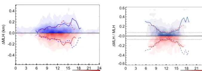
The average agreement is good with a bias of 3.6 m but the overall root mean square error (RMSE) is with 500 m rather large. Figure 1 shows absolute and relative difference between MLH from the Vaisala CT25K and the Jenoptik CHM15k over the course of the day. MLH is mainly detected between 08:00 and 18:00 UTC and the median differences closely follow the zero line over this period. Absolute dif-ferences show a strongly skewed distribution with maximum values larger than 1 km. The first (third) quartile ranges from minimum values around−150 m (+25 m) in the morning and evening hours to−40 m (+150 m) around noon. As they vary with the time of the day relative difference seem to be more adequate for an error estimate. For a fixed time of day the rel-ative differences are – albeit symmetrical – not following a Gaussian distribution. Therefore, instead of a standard devi-ation we consider the 25 and 75 % percentile for the descrip-tion of the uncertainty in the derived aerosol mixing-layer height MLHaero. Over the course of the day these percentiles
are relatively constant and correspond to a relative accuracy of±5 % (Fig. 1).
2.2 Wind lidar
Vertical wind speed is measured with a HALO Photonics Streamline wind lidar (Pearson and Collier, 1999; Pearson et al., 2010; Newsom, 2012). It is a coherent Doppler lidar that uses heterodyne detection to measure the Doppler shift of backscattered light. The instrument is based on a near-infrared lidar system operating at a wavelength of 1.5 µm. The average pulse energy of 100 µJ is larger than the one of the aerosol lidars used in this study as the Doppler retrieval needs more photons to yield reliable results. Laser pulses are emitted at a frequency of 15 kHz and averaged every second. Processing of these data takes some time resulting in a tem-poral resolution of 1.67 s. In its current setup, the maximum range is 8 km but the actual range is limited to areas with sufficient occurrence of aerosol. The spatial resolution along the beam is set to 30 m. Largest and smallest resolvable speed are 19.2 and 0.038 ms−1, respectively. The output consists of wind speed along the beam, backscatter coefficient and SNR from the heterodyne detection. The instrument is equipped with a scanner to point its beam in any direction of the upper hemisphere. In its current setup, it performs several different scan patterns to infer profiles of horizontal wind speed and its spatial distribution. These scans sum up to 12 min per hour. During the remaining 48 min per hour the wind lidar points vertically and measures profiles of vertical velocity.
Unreliable Doppler velocities are filtered by a SNR thresh-old of SNRts=−18.2 dB derived from long-term noise
char-acteristics. This value is somewhat larger than the threshold of−20 dB used by Barlow et al. (2011) based on the consid-erations of Rye and Hardesty (1993). For the instrument used in this study, the value SNRtsindicates the SNR range below
which the Doppler velocity consists only of white noise. It depends on the setup of the instrument, mainly the number of averages, and it differs from instrument to instrument but is relatively constant in space and time.
2.2.1 MLH from vertical wind
From the filtered time series of the vertical velocity, the stan-dard deviationσw is calculated every 5 min from the data
of the surrounding±15 min interval. This standard deviation is corrected for instrumental noise following the technique described by Lenschow et al. (2000). Most of the time the correction is less than a few cm s−1or a few percent ofσw.
The average interval of 30 min is motivated by the considera-tion that a convective plume with an average ascent speed of 1 ms−1needs about 16 min to travel through a mixing layer
of 1 km height. The average interval is thus about twice the life time of such a plume and also typical for the derivation of turbulent fluxes from eddy covariance stations.
As shown by Taylor (1922, 1935) the vertical size of a plume growing due to homogeneous turbulent movement is proportional to σw. We thus use σw as an indicator for
0 3 6 9 12 15 18 21 24 hour (UTC)
0.0 0.5 1.0
∆
MLH (km)
0 20 40 60 80 N/bin
0 3 6 9 12 15 18 21 24 hour (UTC)
-0.2 -0.1 0.0 0.1 0.2
∆
MLH / MLH
0 20 40 60 80 N/bin
Figure 1. Absolute difference1MLH = MLHCT25K−MLHCHM15k(left) and relative difference1MLH/MLHCHM15k(right) of retrieved
MLHaerofrom Vaisala CT25K and Jenoptik CHM15k as function of time of the day for the period 16 August–16 November 2013. Shading shows frequency of occurrence for bin sizes of 30 min and 120 m for absolute and 0.0125 (1.25 %) for relative MLH difference respectively. Red lines are the 25 and 75 % percentile (dashed) and the median (solid) of half hour intervals, respectively. For the analysis 9173 data points were used. During half hour intervals when less than 20 % of the data were available (see text) median and quartiles are not displayed. Dotted lines mark±0.05 chosen as the average error for the MLHaeroestimate.
0 3 6 9 12 15 18 21 24
hour (UTC) -0.4
-0.2 0.0 0.2 0.4
∆
MLH (km)
0 50 100 150 N/bin
0 3 6 9 12 15 18 21 24 hour (UTC)
-0.6 -0.4 -0.2 -0.0 0.2 0.4 0.6
∆
MLH / MLH
01.06.2013 00:00:00 - 02.09.2013 00:00:00
0 50 100 150
N/bin
Figure 2. Absolute change 1MLH = MLH±−MLH0.4 (left) and relative change 1MLH/MLH0.4 (right) of retrieved MLH± for
σwts= (0.4±0.1) ms−1as a function of time of the day. Shading gives the histogram for single retrievals withσwtsincreased (red) and decreased (blue). Bin size is 30 min, 60 m absolute and 0.05 (5 %) relative MLH change. Solid lines are half hour medians for increase (red) and decrease (blue) ofσwts, respectively. Dashed lines are medians mirrored at zero. A total of 8667 (11 218) records have been used for the upper (lower) histograms. During daytime there are on average 440 out of 540 points per half hour interval. Medians are not shown for times when less than 20 % of the original data gave an estimate. Horizontal black dotted lines indicate the±7 % change derived from theσw profile of Lenschow et al. (1980).
whereσw falls below a thresholdσwts. Different thresholds
have been used by Tucker et al. (2009) (σwts= 0.20 and
0.17 ms−1), Pearson et al. (2010) (0.30 ms−1), Barlow et al.
(2011) (0.32 ms−1) and Träumner et al. (2011) (0.40 ms−1). In order to derive a sensible σwtswe make use of the
semi-theoretical profile of Lenschow et al. (1980). This profile is originally based on a handful of airplane measurements but has been recently confirmed with Doppler lidar mea-surements and LES simulations (Lenschow et al., 2012). We assume a typical convective velocity scale of w?= 1.5 ms−1
and arrive at σwts= 0.4 ms−1(see Appendix B and
Träum-ner, 2010). However, in realityw?is time dependent and the
Lenschow et al. (1980) profile is only valid for a developed convective boundary layer. The choice of a threshold method is of course somewhat unsatisfactory as it makes the retrieval
dependent on this value and will be investigated in more de-tail below.
2.2.2 Threshold sensitivity
To investigate the sensitivity of the MLH derived from Doppler lidar to the threshold in σwts a 3-month period
from June to August 2013 was selected andσwts increased
and decreased by 25 % to 0.5 and 0.3 ms−1, respectively.
Times when the wholeσwprofile remained below the
thresh-old were excluded; that mainly concerned night-time data. The histograms (Fig. 2) for the absolute and relative MLH changes due the increase/decrease of σwts show a strong
0.0 0.5 1.0 1.5 2.0 2.5 MLH radiosonde (km) 0.0
0.5 1.0 1.5 2.0 2.5
MLH wind (km)
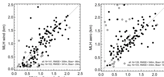
all: N=141, RMSE= 359m, Bias= -86m day: N=102, RMSE= 341m, Bias= -24m
0.0 0.5 1.0 1.5 2.0 2.5
MLH radiosonde (km) 0.0
0.5 1.0 1.5 2.0 2.5
MLH aero (km)
all: N=128, RMSE= 546m, Bias= 209m day: N=103, RMSE= 434m, Bias= 149m
Figure 3. MLHwind(left) and MLHaero(right) versus MLHsondederived from HOPE data during April and Mach 2013. Filled symbols mark
daytime (08:00–16:00 UTC) and open symbols night-time values.
(07:00 UTC) to±150 m (16:00 UTC). It should be noted that both medians lie symmetrically to zero indicating that the av-erageσwshows a linear decrease in this region of the ML.
Figure 2 reveals that best agreement in terms of relative er-ror occurs between 10:00 and 15:00 UTC, i.e. the time frame in which a well-developed convective boundary layer is most likely. Here, the median of the relative differences is quite low and amounts to around 7 %. This is the same value as when using the Lenschow et al. (1980) profile that relates a change in height of±7 % to a change inσw by∓25 % (see
Appendix B). In the morning and afternoon hours the rela-tive difference increases to ±30 %. This indicates that the Lenschow et al. (1980) profile is only valid around noon in the fully developed convective ML. In the morning and af-ternoon hours, the observed σw profiles show a slower
crease with height and consequently the derived MLH de-pends more strongly on the choice of the threshold. We there-fore consider±15 % as error estimate for MLHwind.
2.3 Comparison to radiosonde
To evaluate the remotely sensed MLH retrievals, they are compared to MLHs derived from radio soundings. JOYCE was one of the three central sites of HOPE (High Definition Clouds and Precipitation for advancing Climate Prediction (HD(CP)2) Observational Prototype Experiment, see http: //www.hdcp2.eu/). Two to five radiosondes were launched per day from a site 3.8 km to the southeast of JOYCE dur-ing the 2 month period April–May 2013. From this data set 141 profiles have been used for the comparison. The MLH retrieval from the radiosondes (MLHsonde) was done with
the bulk Richardson number method which is, according to Seibert et al. (2000), the best when also mechanically driven mixing should be detected. This method is based on the as-sumption that an air parcel (or plume) rising from the surface preserves its properties until it reaches a level where it is not buoyant any more and it is destroyed by the wind shear. This level is identified with the critical Richardson number and is
typically slightly above the level of neutral buoyancy. Prior to the retrieval, profiles were smoothed with a five-point glid-ing average which is equivalent to about 50 m. The reference level was chosen to be 60 m in order to avoid effects due to the local micrometeorology. For the critical Richardson num-ber a value of 0.20 was used. MLHwind and MLHaerowere
determined from the 30 min average around the time when the sonde was in the middle of the mixing layer. MLH values below 120 m where rejected as the wind lidar is not sensitive below.
During days with frequent soundings the diurnal course of MLHwindand MLHsondeshow in general good agreement
even during some cases at night when large wind speeds in-duced shear driven mixing. The scatter plot of MLHsonde
ver-sus MLHwind(Fig. 3) shows, apart from some outliers,
differ-ences of less than±500 m. Numerical analysis gives a bias of−86 m and a RMSE of 359 m which is better than the val-ues for MLHaero(209 m and 546 m respectively), or what is
typically found when comparing any aerosol-based retrieval with radio soundings (see e.g. Korhonen et al., 2014; Luo et al., 2014; Haeffelin et al., 2012; Hennemuth and Lammert, 2006). Note that there are some night-time values with espe-cially MLHaerolarger than MLHsondewhen the aerosol-based
algorithm detects the top of (or aerosol layers within) the RL while MLHwind shows good agreement. Omitting these
points from the analysis still gives worse results for MLHaero.
In summary it can be said that MLHwindcompares much
bet-ter to the radiosonde-based MLH than MLHaero.
3 Results
00 03 06 09 12 15 18 21 00 time (UTC)
0.0 0.5 1.0 1.5 2.0 2.5 3.0
height (km)
-3 -2 -1 0 1 2
w (m s
-1)
A
@@
@
@ @ R
B
CC
C
C C
C
CW
C
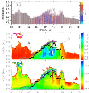
Figure 4. Time–height sections of vertical velocity (top), its standard deviation (stddev, mid panel) and aerosol backscatter coefficient (beta,
bottom panel) on 28 May 2012. MLH retrieved from wind lidar (solid black with diamonds) and from ceilometer (solid grey with triangles). Magenta squares indicate cloud base heights as determined by the ceilometer. Triangles at the abscissa mark sunrise and sunset. Letters A, B and C refer to descriptions in the text. Temporal resolution of the vertical velocity plot is 1 min.
and finally investigate mixing-layer characteristics such as maximum MLH and average growth rate (Sect. 3.3). 3.1 Case study
To investigate the performance of the aerosol-based STRAT-2D compared to the wind-based MLH retrieval, a fair weather spring day (JOYCE, 28 May 2012) with a classical “textbook” boundary layer development is analysed (Fig. 4). Between midnight and 08:00 UTC the residual layer is vis-ible as a region with low values of the standard deviation of vertical velocity (σw<0.20 ms−1) up to approx. 1.5 km.
Convection begins to develop around 06:00 UTC, i.e. 2.5 h after sunrise, as indicated by enhanced σw close to the
sur-face. The MLH steadily increases and reaches the maxi-mum RL height at around 09:00 UTC. At 14:00 UTC the ML reaches its maximum height at about 2.1 km and begins to stagnate. Additionally, starting from 10:30 UTC, cumulus clouds start to develop at the top of the ML visible by the high backscatter and subsequent extinction of the signal above in Fig. 4. Turbulent mixing begins to decay at 16:00 UTC
and collapses almost completely throughout the whole ML at 17:30 UTC, 2 hours before sunset.
Most of the time, both MLH retrievals show good agree-ment. However, some features revealing typical problems of deriving MLH from backscatter profiles can also be ob-served (refer to arrows with letters in Fig. 4). In situation A, the height of the nocturnal boundary layer is interpreted as MLH, althoughσw values are well below 0.1 ms−1. Around
07:00 UTC (situation B), aerosol layers within the RL or at its top around 700 m are erroneously retrieved as MLH, al-though significant mixing is only taking place below 300 m. Finally in situation C (afternoon, starting at 17:00 UTC), the detection of the breakdown of the ML is delayed due to re-maining aerosol particles aloft.
A J J
J J
J J
JJ^ B
A A A A
A A A
A A A A
A A U
C
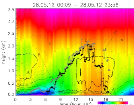
Figure 5. Time–height section of potential temperature from
HAT-PRO (colour shading). Black line with diamonds shows ML from wind, grey line with triangle ML from aerosol. Solid isolines show the vertical potential temperature gradient in steps of 0.5 K/100 m (solid), dotted lines in steps of 0.1 K/100 m between−0.9 K/100 m to +0.9 K/100 m. The thick isoline marks neutral stratification (0 K/100 m). Letters A, B and C refer to descriptions in the text.
the lowest hundred metres of the ABL very accurately with a high resolution of decameters (Löhnert and Meier, 2012). Higher up in the ABL, spatial resolution decreases rapidly, such that the inversion at the top of the boundary layer is usually not resolved.
Potential temperature during night clearly shows the sta-bly stratified and cold nocturnal boundary layer (NBL) with temperatures down to 289 K (04:30 UTC) and gradients of more than+4 K/100 m (01:00–03:00 UTC) close to the sur-face (Fig. 5). The region with pronounced stable stratification grows until 06:00 UTC in the morning (2.5 h after sunrise) when stratification close to the surface quickly transforms from stable to unstable.
During the time span of the lowest temperatures close to the surface, MLHaero increases from 120 m at 03:00 UTC
to around 300 m at 04:30 UTC. However, vertical mixing is very unlikely, as stratification at this time is stable with a strong positive potential temperature gradient. In agreement with this, the Doppler lidar did not detect any significant ver-tical air movement and thus no MLH was assigned (arrow A in Fig. 4). However,β profiles show a region with a signifi-cant vertical gradient leading to the detection of a deepening ML between 03:00 and 05:00 UTC. Most probably this de-velopment was connected to the dissipation of thin mid-level liquid water clouds (base>2.5 km, top<3.2 km as derived from the cloud radar at JOYCE) at 03:00 UTC followed by increased radiative cooling, decreasing temperature (Fig. 5) and increasing relative humidity in the lowest few 100 m. This may have initiated hydrophilic aerosol growth in the
stable NBL and consequently an increasing gradient in the backscatter profiles was interpreted as MLH.
Beginning at 06:00 UTC the ML grew into the NBL, dis-solved it and further grew in the neutrally stratified RL. Be-tween 07:00 and 08:00 UTC the aerosol-derived MLH shows higher values (700 m) than the wind-derived MLH (250 m, arrow B in Figs. 4 and 5). Stratification in this region was still stable and vertical wind as low as during the night. Aerosol backscatter below the wind-derived MLH showed enhanced values. Nevertheless, the gradient inβat this height seems to be lower than gradients in the RL above or even at the top of the RL and these heights are consequently assigned as MLH. The most probable explanation for this behaviour is that with the breakup of the NBL temperature increases, relative humidity decreases and backscatter decreases as well. The backscatter gradient at the top of the ML becomes smaller than gradients in the RL above.
The third situation (arrow C in Figs. 4 and 5) illustrates that the aerosol-based STRAT-2D algorithm cannot follow the breakdown of the MLH around 17:45 UTC. Instead, the top of the aerosol layer, which at this time is the top of the RL, is identified as the MLH. Unfortunately, it is not pos-sible to analyse the temperature inversion at the top of the ABL due to low spatial resolution of the MWR data at these heights. However, Träumner et al. (2011) already noted that incorrect detection during MLH decay is due to the fact that the aerosol distribution in the ABL represents the history of the mixing processes, whereas the vertical wind shows the current status of vertical mixing.
3.2 Average diurnal cycle
After discussing typical issues concerning MLH detection from aerosol backscatter profiles in comparison to the more realistic retrievals from wind lidar in the section above, we now analyse the impacts of the different retrievals on the average diurnal cycle of the MLH. The analysis is carried out over the course of a full year (four seasons) of JOYCE observations between December 2011 and November 2012 (Fig. 6). The winter of the investigated period, especially December and January, were characterized by stormy but relative mild weather, whereas spring and autumn had less precipitation than average, increasing the chance for higher MLHs (Deutscher Wetterdienst, 2011 and 2012).
00 03 06 09 12 15 18 21 time (UTC)
0.0 0.5 1.0 1.5 2.0 2.5 3.0
MLH
aero
(km)
0 250 500
N
00 03 06 09 12 15 18 21
time (UTC) 0.0
0.5 1.0 1.5 2.0 2.5 3.0
MLH
wind
(km)
0 250 500
N
00 03 06 09 12 15 18 21
time (UTC) 0.0
0.5 1.0 1.5 2.0 2.5 3.0
MLH
aero
(km)
0 250 500
N
00 03 06 09 12 15 18 21
time (UTC) 0.0
0.5 1.0 1.5 2.0 2.5 3.0
MLH
wind
(km)
0 250 500
N
00 03 06 09 12 15 18 21
time (UTC) 0.0
0.5 1.0 1.5 2.0 2.5 3.0
MLH
aero
(km)
0 250
N
00 03 06 09 12 15 18 21
time (UTC) 0.0
0.5 1.0 1.5 2.0 2.5 3.0
MLH
wind
(km)
0 250
N
00 03 06 09 12 15 18 21
time (UTC) 0.0
0.5 1.0 1.5 2.0 2.5 3.0
MLH
aero
(km)
0 250
N
00 03 06 09 12 15 18 21
time (UTC) 0.0
0.5 1.0 1.5 2.0 2.5 3.0
MLH
wind
(km)
0 250
N
aerosol
wind
MAM
JJA
SON
DJF
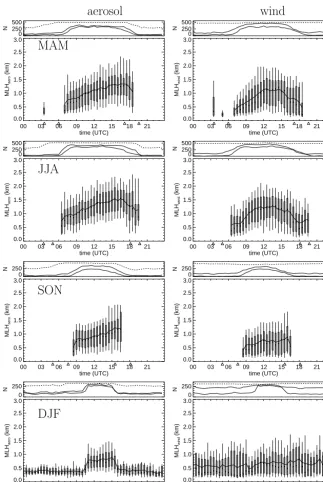
Figure 6. Average diurnal course (solid line) of MLH from aerosol (left panels) and vertical wind (right panels) for spring (MAM), summer
(JJA), autumn (SON) and winter (DJF). Whiskers and boxes indicate 10, 25, 75 and 90 % percentiles. The centre dot indicates the median. On top of every subplot the number of casesNis shown before excluding any data (dashed line), after excluding data below 120 m (solid thin line) and after synchronizing with the other instrument (solid thick line). Triangles at the abscissa mark range of sunrise and sunset during the respective season.
the ceilometer was 40 % (see Table 2). In general data avail-ability from both instruments is similar (see also the number of cases in Fig. 6).
The MLH from both methods show an increase in the morning until noon in spring and summer (MAM and JJA in Fig. 6), which is in general agreement with the com-mon knowledge of the development of a convective boundary
layer (e.g. Stull, 1988). During spring (summer) the average MLHwindbegins to decrease 2 (resp. 3) hours before sunset.
In contrast to this, MLHaeroremains longer at higher MLH
values, decreasing in height with sunset (spring) or 2 hours before the earliest sunset (summer). This behaviour general-izes the difference between MLHwindand MLHaeroalready
00 03 06 09 12 15 18 21 time (UTC)
-1.0 -0.5 0.0 0.5 1.0
∆
MLH (km)
0 250 500
N
00 03 06 09 12 15 18 21
time (UTC) -1.0
-0.5 0.0 0.5 1.0
∆
MLH (km)
0 250 500
N
00 03 06 09 12 15 18 21
time (UTC) -1.0
-0.5 0.0 0.5 1.0
∆
MLH (km)
0 250
N
00 03 06 09 12 15 18 21
time (UTC) -1.0
-0.5 0.0 0.5 1.0
∆
MLH (km)
0 250
N
MAM JJA
SON DJF
Figure 7. Difference1MLH = MLHaero−MLHwindfor the four seasons. Whiskers and boxes indicate 10, 25, 75 and 90 % percentiles
and dots indicate the median. Red lines indicate average (solid) and the error estimate based on the sensitivity studies in Sects. 2.1.4 and Sect. 2.2.2 (dashed). Triangles at the abscissa mark range of sunrise and sunset during the respective season.
0.3 0.6 0.9 1.2 1.5 1.8 2.1 2.4 2.7 3.0 3.3 3.6
mlhmax (km)
0 10 20 30 40 50 60
frequency (%)
N=81 N=81
0.3 0.6 0.9 1.2 1.5 1.8 2.1 2.4 2.7 3.0 3.3 3.6
mlhmax (km)
0 10 20 30 40 50 60
frequency (%)
N=54 N=54
0.3 0.6 0.9 1.2 1.5 1.8 2.1 2.4 2.7 3.0 3.3 3.6
mlhmax (km)
0 10 20 30 40 50 60
frequency (%)
N=52 N=52
0.3 0.6 0.9 1.2 1.5 1.8 2.1 2.4 2.7 3.0 3.3 3.6
mlhmax (km)
0 10 20 30 40 50 60
frequency (%)
N=50 N=53
MAM
JJA
SON
DJF
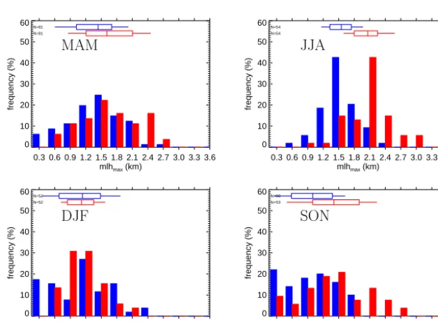
Figure 8. Frequency of occurrence of maximum MLH from wind lidar (blue) and ceilometer (red) for spring, summer, autumn and winter
(clockwise from top left). Whisker boxes on top show 10, 25, 75 and 90 % percentiles and the median.
the morning hours before noon, average MLHaerois in
gen-eral larger and shows a smaller growth rate than MLHwind.
This could be related to situations denoted as B in the case study above (Figs. 4 and 5). In winter (DJF), night-time val-ues above the minimum ML are frequently retrieved by both methods. This is due to a rather large number of storm pas-sages in the winter data set. The observed large nocturnal
mixing-layer heights are thus not convectively driven, but caused by wind shear. Switching of the STRAT-2D algorithm between the day mode (beginning 3 h after sunrise) and the night mode (beginning with sunset) is in winter clearly vis-ible as a sudden increase in MLHaero. In contrast, MLHwind
1 3 5 7 9 11 13 15 17 19 21 23
hourmax (UTC)
0 10 20 30 40 50 60
frequency (%)
N=81 N=81
1 3 5 7 9 11 13 15 17 19 21 23
hourmax (UTC)
0 10 20 30 40 50 60
frequency (%)
N=54 N=54
1 3 5 7 9 11 13 15 17 19 21 23
hourmax (UTC)
0 10 20 30 40 50 60
frequency (%)
N=48 N=51
1 3 5 7 9 11 13 15 17 19 21 23
hourmax (UTC)
0 10 20 30 40 50 60
frequency (%)
N=52 N=52
MAM
JJA
SON
DJF
Figure 9. Frequency of occurrence of time of the day when maximum MLH is reached for wind lidar (blue) and ceilometer (red) derived
MLH. Clockwise from top left: spring, summer, autumn and winter. Whisker boxes on top show 10, 25, 75 and 90 % percentiles and the median.
30 90 150 210 270 330 390 450 510
growth rate (m h-1
) 0
10 20 30 40 50 60
frequency (%)
N=66 N=65
30 90 150 210 270 330 390 450 510
growth rate (m h-1
) 0
10 20 30 40 50 60
frequency (%)
N=47 N=45
30 90 150 210 270 330 390 450 510
growth rate (m h-1
) 0
10 20 30 40 50 60
frequency (%)
N=31 N=36
30 90 150 210 270 330 390 450 510
growth rate (m h-1
) 0
10 20 30 40 50 60
frequency (%)
N=29 N=32
MAM
JJA
SON
DJF
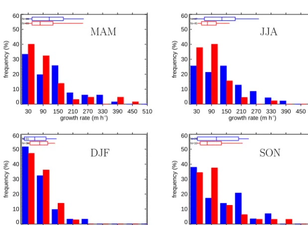
Figure 10. Frequency of occurrence of average growth rate of MLH between sunrise and time when 90 % of MLHmaxis reached. Clockwise
from top left are shown spring, summer, autumn and winter. Whisker boxes on top show 10, 25, 75 and 90 % percentiles and the median.
the switching of STRAT-2D between night and daytime is not working properly at least in winter time.
In general, the difference1MLH=MLHaero−MLHwind
is positive for all seasons except for night-time in winter (Fig. 7). This is as expected, as the wind retrieval of a Doppler wind lidar depends on aerosol backscatter. They should be equal in the case of a fully developed ML above
which only clean air of the free troposphere and thus no backscatter can be found. In the case of a developing ML, which grows into the RL, there might be aerosol above and MLHaerocould be larger than MLHwind. In contrast, the
com-parison by Pearson et al. (2010) showed MLHwind to be
larger than MLHaerobut as their measurements were taken in
00 03 06 09 12 15 18 21 00 time (UTC)
0.0 0.5 1.0 1.5 2.0 2.5 3.0
z (km)
0.0 0.2 0.4 0.6 0.8 1.0
frequency (%)
00 03 06 09 12 15 18 21 00
time (UTC) 0.0
0.5 1.0 1.5 2.0 2.5 3.0
z (km)
0.0 0.2 0.4 0.6 0.8
frequency (%)
00 03 06 09 12 15 18 21 00
time (UTC) 0.0
0.5 1.0 1.5 2.0 2.5 3.0
z (km)
0.0 0.2 0.4 0.6 0.8 1.0
frequency (%)
00 03 06 09 12 15 18 21 00
time (UTC) 0.0
0.5 1.0 1.5 2.0 2.5 3.0
z (km)
0.0 0.2 0.4 0.6 0.8
frequency (%)
MAM JJA
SON DJF
Figure 11. Frequency of occurrence of cloud bases (shading) and overlaid ML from ceilometer (red) and wind lidar (blue) with cloudy cases
excluded. Bin size is 90 m×1 h. Cloud base heights are excluded from half hour intervals when cloud coverage was larger than 4 octa.
Table 3. Seasonal medians of daily maximum MLH (max), time of maximum (hmax) and growth rate (GR) of MLH for JOYCE, December
2011–November 2012.
Wind Aerosol
MAM JJA SON DJF MAM JJA SON DJF
max (km) 1.4 1.6 1.0 1.1 1.6 2.1 1.4 1.1
hmax(hour UTC) 13.6 13.0 12.8 11.9 15.1 15.8 13.3 13.5
GR (m h−1) 115 131 109 56 78 73 72 76
properties. From our study it is obvious that on average MLHwind≤MLHaeroholds.
The spread of the differences between both MLHs, de-picted by the 25 and 75 % percentiles, is rather large with values up to 500 m (Fig. 7) but in the same order of magni-tude as the differences found when comparing to radioson-des (see Sect. 2.3). The spread is largest in the afternoon and larger in summer than in spring and autumn. Considering the error estimate based on the sensitivity studies in Sects. 2.1.4 and Sect. 2.2.2 the differences are significant most of the time, particularly in the late afternoon in spring, summer and autumn (Fig. 7). As this difference cannot be removed by changing the threshold σwtswithin the large range
investi-gated in Sect. 2.2.2 it must be concluded that MLHaero is
systematically overestimated.
In spring, summer and autumn, mean and median of
1MLH show the same behaviour: larger differences in the morning and afternoon hours and values closer to zero around noon. The overestimation of MLHaerois strongest in
the morning and the late afternoon during these seasons. The largest differences occur in the late afternoon reaching aver-age and median values of 600 m which is in the order of the
MLH itself at that time of the day. Similarly, in the morn-ing, the difference in MLH is of the order of 300 m. This pattern of MLH differences does not appear during winter (DJF) when convective conditions are rather rare.
3.3 Mixing-layer characteristics
The daily development of the ML can be characterized by three parameters: the maximum height (MLHmax), the time
when this height is reached (hourmax) and the rate at which
the ML is growing in the morning hours (GR). As MLHaero
is larger than MLHwindin the morning and late afternoon, we
can expect that there will be systematic differences in the ML characteristics from the two instruments.
For the determination of the daily maximum of MLH, both data sets MLHaeroand MLHwindare smoothed with a 1-hour
gliding average to avoid outliers to be taken as the maximum. The growth rate is determined similar to Baars et al. (2008) and Korhonen et al. (2014) as the slope of a linear fit to the data between the first reported MLH after sunrise and the time when 90 % of the maximum is reached. It is thus an average growth rate.
As for the half-hourly averages, the largest maximum MLHs are observed in summer and maxima are larger in spring than in autumn (Fig. 8 and Table 3). Winter values are rather high which is again related to the stormy win-ter with several days with shear-induced mixing. A com-parison with MLHwind reveals a systematic overestimation
by the aerosol-based retrieval which is with 500 m largest in summer, smaller in spring (200 m) and autumn (400 m) and negligible only in winter. Medians of the seasonal max-imum MLHaeroare by about 300 m larger than those values
from Baars et al. (2008) for Leipzig, a central European site, whereas MLHwind agrees very well for spring and autumn
and even the difference in summer is lower than the uncer-tainty due to day-to-day variability. Values are also compa-rable to those found by Granados-Muñoz et al. (2012) at a site in southern Spain. They are larger than those reported by Chen et al. (2001) for a city in Japan which is probably due to the more moist climate and thus a lower surface sensible heat flux. As one could expect, they are lower than those found by Korhonen et al. (2014) in South Africa at a lower latitude in a drier climate.
The median of the time when the maximum MLHwindis
reached is for all seasons, except winter, around 13:00 UTC i.e. 1.3 hours after local noon (Fig. 9). The quartiles indi-cate that, except in winter, more than half of the cases are within ±2 hours of this time while the time of maximum MLHaero occurs in spring and summer by about 2.5 hours
later than that of MLHwind. In winter, shear-induced
mix-ing leads to MLH maxima durmix-ing night which are only de-tected by MLHwind. Both results, the larger and the later
max-imum of MLHaero, can be explained by the incapability of
the aerosol-based retrieval to capture the termination of con-vection, i.e. when MLHaeroshows a still growing ML, while
the vertical wind indicates no more mixing. Nevertheless, it remains unclear why MLHaerois growing although the
ver-tical wind indicates no mixing connected to the surface. A possible reason could be shear-induced mixing at the top of the residual layer which would dilute aerosol into the free
troposphere and thus lift the region with the most significant gradient.
Mean growth rates of MLHwind are largest in summer
with 50 % of the days showing values larger than 131 m h−1 (Fig. 10). Growth rates in spring are larger than those in autumn which is similar to the observed larger maxima in spring compared to autumn. In winter, growth rates are in general smaller and often lie below 120 m h−1. The distri-bution is during all seasons positively skewed with largest values around 390 m h−1. The 1-year statistics derived by Baars et al. (2008) and Korhonen et al. (2014) are both also skewed but show larger values (up to 600 m h−1) and also lesser values below 100 m h−1. This might be related to the fact that both studies are restricted to cases with no bound-ary layer clouds and thus higher insolation, higher convec-tive activity and thus less small growth rates. The fact that they had to restrict their analysis to times when the MLH reaches the height with sufficient lidar overlap, i.e. 300 m, may also play a role: this restriction excludes the morning hours of slow MLH growth when the NBL is dissolved. The MLHaero-based growth rates are in general lower than those
of MLHwindwith the median between 37 m h−1(spring and
autumn) and 58 m h−1lower (see Table 3). This behaviour can be explained by the tendency of the aerosol-based re-trieval to detect the top of, or layers within, the residual layer, especially in the morning hours. This results in larger morn-ing MLHs and thus in lower average growth rates.
3.4 Connection of ML to clouds
Cumulus clouds are directly connected to the atmospheric boundary layer as they are the convective plumes which be-come visible due to condensation. To investigate this further we compare here cloud bases as detected by the ceilometer with the MLH found by the two methods. We use the data set with cloud cover below 3 km lower than 4 octa. Although this does not fully guarantee that the observed clouds are cu-mulus clouds, we regard it as a first attempt to restrict to this cloud class.
Figure 11 shows a 2-D histogram of cloud base heights (CBH) with the average MLHs from aerosol- and wind-based retrieval overlaid. Cloud bases are those reported every 15 s by the Vaisala ceilometer. The cloud base statistic is similar to what Brümmer et al. (2012) found in a 7-year statistic from a site near Hamburg about 380 km to the northeast of JOYCE under similar climatic conditions (Fig. 18 in Brümmer et al., 2012). A similar pattern can also be found in the Climate Modeling Best Estimate data set derived from a continental site (CMBE, Fig. 3a in Xie et al., 2010).
Table 4. Comparison of the capabilities of the MLH retrievals in different situations. AL, aerosol layer; ML, mixing layer; NBL, nocturnal
boundary layer; RL, residual layer.
Situation Ceilometer Wind lidar
Night −− detects ALs, NBL or top of RL + intermittent turbulence?
Growing ML ◦ no gradient between ML and RL ++ clear difference between ML and RL
Fully developed ML ++ top of ML coincides with top of AL ++ strong turbulence over whole ML
Evening decay − sticks to top of aerosol layer + sees decaying mixing
which might be related to dissolving stratus clouds. In win-ter highest frequencies for cloud bases are in the lowest few hundred metres, which might be related to fog.
The strong connection between MLH and CBH in spring and summer coincides with the general experience that the base of cumulus clouds is located always more or less at the top of the boundary layer but never significantly below and of course never above (see e.g. studies on shallow trade wind cumulus – Riehl et al., 1951; Augstein et al., 1974). The mechanism can be described as follows: the ML grows until it reaches the cumulus condensation level (CCL) and cumulus clouds form. Incident solar radiation at the surface is reduced, convection becomes weaker and ML growth is reduced. Warming and drying of the ML lifts the CCL and cloud cover is reduced. Incident solar radiation and thus con-vection increases and again influences the cloud cover. Sev-eral studies used large eddy simulation (LES) to understand the role of the different fluxes in the mass and heat budget of the cumulus topped ABL (see e.g. Brown et al., 2002). Oth-ers investigate mass flux schemes suitable for climate models (e.g. Neggers et al., 2004). All these model studies show that there is a strong coupling between CCL and MLH.
As the determination of CBH is much simpler than the de-termination of MLH it could be used as a good proxy for MLH. Nevertheless, it is necessary to ensure that the ob-served clouds are convective, e.g. by investigating the surface sensible heat fluxHs. This could be done in a multi-sensor
approach as proposed e.g. in the boundary layer classifica-tion by Harvey et al. (2013), or in a simpler way by checking in situations with sufficiently largeHs, whether MLHaerolies
close to CBH.
4 Summary and conclusions
We analysed and compared 1 year of MLHs derived from (i) aerosol backscatter and (ii) standard deviation of the ver-tical wind speed. To our knowledge this is the first long-term evaluation of vertical wind derived MLH. For (i) we used backscatter data from a Vaisala CT25K ceilometer and the STRAT-2D algorithm with its core based on an edge de-tection algorithm (Sect. 2.1). For (ii) we used vertical wind speed data from a HALO Photonics streamline wind lidar and a threshold algorithm (Sect. 2.2). The basic idea is that the vertical velocity is a direct measure of the turbulent
mix-ing, while in contrast the backscatter profile is only a proxy for the mixing process.
A comparison with 141 MLHs from radiosonde profiles showed better agreement with the wind-derived MLH than the aerosol-derived MLH (Sect. 2.3).
The uncertainty of the MLH retrieval from aerosol was estimated to be 5 % by comparing MLHs from the Vaisala CT25K ceilometer with those from a more powerful Jenoptik CHM15K ceilometer (Sect. 2.1.4). The MLH retrieval from the vertical wind is based on a threshold for the standard de-viationσw of the vertical wind. Although the choice of the
threshold can be justified by the semi-theoreticalσw profile
of Lenschow et al. (1980) by assuming an average convec-tive velocity scalew?, it is somewhat arbitrary. An alternative
could be to search for the height where theσw profile falls
below a certain fraction of its maximum. This fraction could be derived from e.g. the Lenschow et al. (1980) profile (see equation B6), but from our experience especially the morning and late afternoon profiles deviate substantially from the the-oretical profile (see also Sect. 2.2.2). As a result this method is less robust than the threshold method and we could show that a large change of the threshold by 25 % changes the re-trieved MLH by only 15 % (Sect. 2.2.2).
The evaluation of the 1-year data shows that in general MLHs from both methods follow the typical evolution of a convective growing mixing layer. However, the method based on aerosol backscatter profiles typically overestimates the MLH throughout the day, and especially cannot follow the mixing-layer evolution in the morning and late afternoon hours (Sect. 3.2). This confirms earlier findings for aerosol-based MLH retrieval of the growing ML in the morning (e.g. Eresmaa et al., 2012) and its evening decay (e.g. Träumner et al., 2011). For the first time, the present study quantifies the average error of an aerosol-based MLH retrieval on a half-hourly basis. It is lowest (of the order of 100 m) around noon and has distinct maxima in the morning (of the order of 300 m) when the ML grows into the residual layer (RL) and in the late afternoon (of the order of 600 m) when turbulence decays.
remaining aerosol layers within the RL. This also explains why the morning overestimate is smaller than in the after-noon.
In the late afternoon when turbulence decays, aerosol par-ticles still remain well mixed and no clearly detectable gradi-ent at the top of the descending mixing-layer top can be iden-tified. Instead, any aerosol-based algorithm will continue to identify the top of the aerosol layer as MLH, which at this time of the day is already the top of the RL (situation C in Fig. 4).
Table 4 summarizes the performance of the two meth-ods on days with convection and low cloud cover or clear sky conditions. Our analysis indicates that retrieving MLH with the backscatter-based method is more challenging than with the vertical velocity-based method. Although a MLH retrieval based on vertical wind seems at first sight simple there are some principal restrictions to be mentioned. During night vertical movement is suppressed in the stably stratified NBL. Nevertheless, strong wind shear due to e.g. the noctur-nal low-level jet may lead to intermittent turbulence which is an occasional and locally constricted event (Van de Wiel et al., 2003). These events can cause effective mixing be-tween layers, but might be missed with a vertically pointing instrument which can see only events at its own location.
Likewise, the late afternoon decay of the convective turbu-lence is a transition to a more intermittent regime, i.e. plumes which reach the top of the ML become less frequent. As a resultσwdecays only gradually with time and the exact
mo-ment when the retrieval reports the breakdown of convective mixing depends strongly on the threshold. Due to the inter-mittent nature of the turbulence the standard deviation of ver-tical wind speed fluctuates in time and the retrieved MLH may jump between low and high values if the fluctuation is around the threshold. We also observed late afternoon cases when active plumes were advected in the upper two-thirds of the ABL only, while the lower third was calm. The retrieval then reported no MLH as no mixing between the surface and the layers above occurred. However, these cases are rare and in general the decay ofσw occurs similarly at all levels. In
summary it can be said that it is principally not possible to determine the exact moment of the end of convective mixing and a differentσwthreshold may shift the moment of
detec-tion. Nevertheless, a reduction of theσwthreshold by 25 % is
not sufficient to explain the difference between aerosol- and wind-derived MLH.
The systematic overestimation of MLH by the aerosol-based retrieval especially in the morning and afternoon hours has its effects on derived seasonal average ML characteristics: the aerosol-based MLH shows a maximum (+200, . . . ,+500 m) higher than that from the wind. It is reached on average 2.5 h later in the afternoon and aver-age growth rates are smaller when compared with the wind-derived MLH. A comparison of the seasonal MLH maxima with those found by Baars et al. (2008) in Leipzig, cen-tral Europe, under similar climatic conditions, reveals
sys-tematically larger MLHs from the ceilometer whereas the wind-derived MLHs agree very well. Nevertheless, differ-ences are smaller than day-to-day variability. Average MLH growth rates are smaller than those reported by Baars et al. (2008) but this might be related to their retrieval: their data set was restricted to cloud-free conditions and due to the overlap function of their lidar they had to restrict to MLHs larger than 300 m. Both of these restrictions prefer situations with higher growth rates, making a comparison difficult. Be-side these retrieval-related differences it is unclear how large the year-to-year variability of MLH characteristics is. Many parameters influence the MLH development. Water vapour content and night-time cloud cover determine radiative cool-ing and thus how deep and how cold the NBL becomes and how long it takes to dissolve the NBL. Cloud cover dur-ing daytime strongly modulates the incomdur-ing solar radiation and thus energy available for ML growth. More precipitation means higher soil moisture, a higher latent heat flux at the surface at the cost of the sensible heat flux, and thus less in-tensive convection and lower MLHs. Another important pa-rameter is the stratification of the free troposphere which lim-its growth rate and maximum height of the fully developed mixing layer.
As described by White et al. (2009), state-of-the-art dis-persion models could be significantly improved by provid-ing measured MLH as input. Ceilometers are widespread, e.g. at airports, and can provide continuous MLH estimates in networks (Haij et al., 2007; Haeffelin et al., 2012). We could show that aerosol-based MLH estimates suffer from systematical overestimation of the order of several hundred metres, especially in the morning and late afternoon hours when emissions from road traffic are largest. Concentrations of surface emitted pollutants in the mixing layer scale di-rectly with the height of the ML. Accordingly, this overes-timation significantly alters predictions of concentrations to-wards too low values.
Appendix A: Comparing ceilometers
The key parameters to describe a lidar are wavelengthλ, en-ergy per pulse E0, number of pulses averaged to one
pro-fileNP, opening area of the receiving telescope (apertureA),
range gate length (1r) and beam diameter (D). The receiver is usually an avalanche photodiode (APD, the semiconduc-tor equivalent to a photomultiplier) which in principle counts single photons. Thus the number of typically sent and re-ceived photons is a good measure to compare two instru-ments.
The number of emitted photonsN0is the energy per pulse
EP divided by the energy per photonE0which depends on
wavelengthλ(Planck’s relation):E0=h·c/λ, with Planck’s
constanthand speed of lightc, and thusN0=EP·λ/(h·c).
For the average profile, Nm=N0·NP photons are emitted.
Comparing two instruments AandB the relation between the emitted photons is
NmA
NmB
= EPA ·λA·NPA
EPB·λB·NPB
. (A1)
The number of backscattered photonsNβ depends on the
wavelength and the type of aerosol. The wavelength depen-dence can be estimated by a power law: Nβ∼λ−νmie with
Angstrom exponentνmiewhich is for continental aerosol
typ-ically of the order of 1, . . . ,1.8. The number also depends on the number of scattering particles and thus on size of the vol-ume, i.e. range gate length 1r, and square of the beam di-ameterD, i.e.Nβ∼1r·D2. Finally, only those photons that
reach the telescope have a chance to be counted by the APD, thus it must be proportional to the aperture (A). We thus get for the received photonsNr:
NrA
NrB
= EPA ·λ
1−νmie
A ·NPA·1rA·D
2 A
EPB·λ1
−νmie
B ·NPB·1rB·D2B
. (A2)
Of course this estimate does not take into account the further pathway within the instrument, i.e. transmittance of the op-tics, bandwidth of the filters, sensitivity and dynamic range of the receiver, etc.
We operate two ceilometers at JOYCE: a Vaisala CT25K and a Jenoptik CHM15k with parameters depicted in Table 1. Although the Jenoptik emits nearly ten times more photons the number of potentially received photons per range gate is only 4.4 times larger than for the Vaisala. The main loss is due to the shorter range gate length. As the Jenoptik shows in general a much better sensitivity and less noise, it can be concluded that the receiver is better.
Appendix B: The Lenschow profile
Lenschow et al. (1980) derived a universal profile for σw
based on a handful of airplane measurements and scaling considerations. Scaling parameter for height should be the height of the convective mixing layerh. Velocity should scale with the convective velocity scale proposed by Deardorff (1970). Close to the surface the height dependence should be of the form(z/ h)1/3, at the surfaceσwshould be zero and
the profile should have a maximum in the lower half of the convective mixing layer leading to the following form:
σw =w?·c1·ζν ·(1−c2·ζ )µ (B1)
withζ=z/ h the height scaled with mixing-layer height h
and parametersc1=
√
1.8 = 1.34,c2= 0.8,ν=13andµ= 1. At
the top of the ML, atζ= 1, the profile does not become zero – it is
σwtop =w?·c1·(1−c2)µ=0.268·w?. (B2)
The derivative with respect toζ is
∂σw
∂ζ =σw ·
ν
ζ − c2
1−c2ζ
. (B3)
At the maximum the derivative is zero, leading to
ζmax=
ν c2·(µ+ν)
=0.312. (B4)
The valueσwmaxat this height is
σwmax =w?·c1·ζmaxν ·(1−c2·ζmax)µ =0.682·w?. (B5)
The value at ML top can be expressed relative to the value of the maximum:
σwtop =
1
ζν max
·
1−c
2
1−c2·ζmax
µ
=0.393·σwmax. (B6)
The profile can also be utilized to estimate the depen-dence of the MLH estimate from the threshold. Using
∂σw
∂ζ 1
σw'
1σw
σw
h
1z at mixing-layer top (ζ= 1) the relative
change of determined MLH with a relative change of thresh-oldσwtsbecomes
1MLH
MLH =
1
ν− c2
1−c2
· 1σwts
σwts
= −0.273· 1σwts
σwts
. (B7)
That means that with an increase (decrease) of
σwts= 0.4 ms−1 by 0.1 ms−1 (i.e. 25 %) the detected
Acknowledgements. We gratefully acknowledge financial support
by the SFB/TR 32 “Pattern in Soil-Vegetation-Atmosphere Sys-tems: Monitoring, Modelling, and Data Assimilation” funded by the Deutsche Forschungsgemeinschaft (DFG). Work by A. Hirsikko was supported within the project High Definition Clouds and Pre-cipitation for advancing Climate Prediction HD(CP)2 funded by the German Ministry for Education and Research (BMBF) under grant FK 01LK1209B. Radiosonde data came from the HOPE-experiment which is part of the HD(CP)2 project (BMBF grant 01LK1212F). We thank Martin Kohler for providing these data.
We thank Kerstin Ebell for proofreading the paper.
Edited by: L. Bianco
References
American Meteorological Society: Glossary of Meteorology, Amer-ican Meteorological Society, http://glossary.ametsoc.org/, last access: 25 April 2014, 2013.
Augstein, E., Schmidt, H., and Wagner, V.: The vertical structure of the atmospheric planetary boundary layer in undisturbed Trade winds over the Atlantic Ocean, Bound-Lay. Meteorol., 6, 129– 150, doi:10.1007/BF00232480, 1974.
Baars, H., Ansmann, A., Engelmann, R., and Althausen, D.: Con-tinuous monitoring of the boundary-layer top with lidar, At-mos. Chem. Phys., 8, 7281–7296, doi:10.5194/acp-8-7281-2008, 2008.
Banta, R. M., Pichugina, Yelena, L., and Brewerm, W. A.: Turbulent Velocity-Variance Profiles in the Stable Boundary Layer Gener-ated by a Nocturnal Low-Level Jet, J. Atmos. Sci., 63, 2700– 2719, doi:10.1175/JAS3776.1, 2006.
Barlow, J., F., Dunbar, T. M., Nemitz, E. G., Wood, C. R., Gallagher, M., Davies, F., O’Connor, E., and Harrison, R. M.: Boundary layer dynamics over London, UK, as observed using Doppler li-dar during REPARTEE-II, Atmos. Chem. Phys., 11, 2111–2125, doi:10.5194/acp-11-2111-2011, 2011.
Brooks, I.: Finding boundary layer top: application of a wavelet covariance transform to lidar backscatter profiles, J. Atmos. Ocean. Tech., 20, 1092–1105, doi:10.1175/1520-0426(2003)020<1092:FBLTAO>2.0.CO;2, 2003.
Brown, A., Chlond, A., Golaz, C., Khairoutdinov, M., Lewellen, D., Lock, A., MacVean, M., Moeng, C.-H., Neggers, R., Siebesma, A., and Stevens, B.: Large-eddy simulation of the diurnal cycle of shallow cumulus convection over land, Quat. J. Roy. Mete-orol. Soc., 128, 1075–1094, doi:10.1256/003590002320373210, 2002.
Brümmer, B., Lange, I., and Konow, H.: Atmospheric boundary layer measurements at the 280 m high Hamburg weather mast 1995–2011: mean annual and diurnal cycles, Meteorologische Zeitschrift, 21/4, 319–335, doi:10.1127/0941-2948/2012/0338, 2012.
Canny, J.: A Computational Approach to Edge Detection, IEEE Transactions on Pattern Analysis and Machine Intelligence (PAMI), 8, 679–698, doi:10.1109/TPAMI.1986.4767851, 1986. Chen, W., Kuze, H., Uchiyama, A., Suzuki, Y., and Takeuchi, N.:
One-year observation of urban mixed layer characteristics at Tsukuba, Japan using a micro pulse lidar, Atmos. Environ., 35, 4273–4280, doi:10.1016/S1352-2310(01)00181-9, 2001.
Cimini, D., De Angelis, F., Dupont, J.-C., Pal, S., and Haeffelin, M.: Mixing layer height retrievals by multichannel microwave radiometer observations, Atmos. Meas. Tech., 6, 2941–2951, doi:10.5194/amt-6-2941-2013, 2013.
Cohn, S. A. and Angevine, W. M.: Boundary Layer Height and Entrainment Zone Thickness Measured by Lidars and Wind-Profiling Radars, J. Appl. Meteorol., 39, 1233–1247, doi:10.1175/1520-0450(2000)039<1233:BLHAEZ>2.0.CO;2, 2000.
Collier, C., Davies, F., Bozier, K., Holt, A., Middleton, D., Pearson, G., Siemen, S., Willetts, D., Upton, G., and Young, R.: Dual-Doppler Lidar Measurements for Improving Dispersion Models, B. Am. Meteorol. Soc., 86, 825–838, doi:10.1175/BAMS-86-6-825, 2005.
Davis, K., Gamage, N., Hagelberg, C., Kiemle, C., Lenschow, D., and Sullivan, P.: An objective method for deriving atmospheric structure from airborne lidar observations, J. Atmos. Ocean. Tech., 17, 1455–1468, doi:10.1175/1520-0426(2000)017<1455:AOMFDA>2.0.CO;2, 2000.
Deardorff, J.: Convective Velocity and Temperature Scales for the Unstable Plantery Boundary Layer and for Rayleigh Con-vection, J. Atmos. Sci., 27, 1211–1213, doi:10.1175/1520-0469(1970)027<1211:CVATSF>2.0.CO;2, 1970.
Deutscher Wetterdienst: Witterungsreport, 2011 and 2012. Emeis, S., Schäfer, K., and Münkel, C.: Surface-based remote
sensing of the mixing-layer height – a review, Meteorologische Zeitschrift, 17, 621–630, doi:10.1127/0941-2948/2008/0312, 2008.
Endlich, R., Ludwig, F., and Uthe, E.: An automatic method for determining the mixing depth from lidar observations, Atmos. Environ., 13, 1051–1056, doi:10.1016/0004-6981(79)90015-5, 1979.
Eresmaa, N., Karppinen, A., Joffre, S., Räsänen, J., and Talvitie, H.: Mixing height determination by ceilometer, Atmos. Chem. Phys., 6, 1485–1493, doi:10.5194/acp-6-1485-2006, 2006. Eresmaa, N., Härkönen, J., Joffre, S., Schultz, D., Karppinen, A.,
and Kukkonen, J.: A Three-Step Method for Estimating the Mix-ing Height UsMix-ing Ceilometer Data from the Helsinki Testbed, J. Appl. Meteorol. Climatol., 51, 2172–2187, doi:10.1175/JAMC-D-12-058.1, 2012.
Garratt, J.: The Atmospheric Boundary Layer, Cambridge Univer-sity Press, Cambridge, England, 1994.
Granados-Muñoz, M. J., Navas-Guzmán, F., Bravo-Aranda, J. A., Guerrero-Rascado, J. L., Lyamani, H., Fernández-Gálvez, J., and Alados-Arboledas, L.: Automatic determination of the plane-tary boundary layer height using lidar: One-year analysis over southeastern Spain, J. Geophys. Res. Atmos., 117, D18208, doi:10.1029/2012JD017524, 2012.
Haeffelin, M., Angelini, F., Morille, Y., Martucci, G., Frey, S., Gobbi, G. P., Lolli, S., O’Dowd, C. D., Sauvage, L., Xueref-Rémy, I.AND Wastine, B., and Feist, D. G.: Evaluation of Mixing-Height Retrievals from Automatic Profiling Lidars and Ceilometers in View of Future Integrated Networks in Europe, Bound-Lay. Meteorol., 143, 49–75, doi:10.1007/s10546-011-9643-z, 2012.