www.atmos-meas-tech.net/7/3935/2014/ doi:10.5194/amt-7-3935-2014
© Author(s) 2014. CC Attribution 3.0 License.
Assimilation of GNSS radio occultation observations in GRAPES
Y. Liu1,3and J. Xue2
1Numerical Weather Prediction Center, China Meteorology Administration, Beijing, 100081, China
2State Key Laboratory of Severe Weather, Chinese Academy of Meteorological Sciences, China Meteorology Administration, Beijing 100081, China
3National Meteorological Center, China Meteorological Administration, No. 46 South Zhongguancun Street, Haidian District, Beijing 100081, China
Correspondence to: Y. Liu (liuyan@cma.gov.cn)
Received: 19 May 2014 – Published in Atmos. Meas. Tech. Discuss.: 24 July 2014 Revised: 14 October 2014 – Accepted: 15 October 2014 – Published: 26 November 2014
Abstract. This paper reviews the development of the global navigation satellite system (GNSS) radio occultation (RO) observations assimilation in the Global/Regional Assimila-tion and PrEdicAssimila-tion System (GRAPES) of China Meteoro-logical Administration, including the choice of data to as-similate, the data quality control, the observation operator, the tuning of observation error, and the results of the obser-vation impact experiments. The results indicate that RO data have a significantly positive effect on analysis and forecast at all ranges in GRAPES, not only in the Southern Hemisphere where conventional observations are lacking but also in the Northern Hemisphere where data are rich. It is noted that a relatively simple assimilation and forecast system in which only the conventional and RO observation are assimilated still has analysis and forecast skill even after nine months integration, and the analysis difference between both hemi-spheres is gradually reduced with height when compared with NCEP (National Centers for Environmental Prediction) analyses. Finally, as a result of the new on-board payload of the Chinese FengYun-3 (FY-3) satellites, the research status of the RO of FY-3 satellites is also presented.
1 Introduction
The RO is an innovative limb sounding technique for probing the atmosphere. It was originally used to investigate the at-mosphere of Mars in the early 1960s (Fjeldbo and Eshleman, 1968); however, it was not used to probe the Earth’s atmo-sphere for two reasons. First, RO observations require both a radio source and a suitable receiver off the planet and
out-side the atmosphere; such matched pairs were not available in Earth’s orbit. Second, we have much information regarding the Earth; as a result, if the RO measurements cannot provide atmospheric information at the synoptic scale, they will have no additional value (Yunck, 2002).
The proof-of-concept mission GPS/MET (Global Posi-tioning System/Meteorology) in 1995 began a revolution in experiments using radio occultation to profile the Earth’s atmosphere (Ware et al., 1996; Kursinski et al., 1997; Rocken et al., 1997). Subsequently, CHAMP (CHAlleng-ing Minisatellite Payload), SAC-C (Satellite de Aplica-ciones Cientificas-C), GRACE (Gravity Recovery and Cli-mate Experiment), METOP-A and -B, TerraSAR-X, and FORMOSAT-3/COSMIC (Formosa Satellite mission 3/Con-stellation Observing System for Meteorology, Ionosphere, and Climate, referred to as COSMIC hereafter) all demon-strated the capabilities of radio occultation for probing the Earth’s atmosphere accurately (Anthes, 2011).
The RO technique can precisely measure the delay of a ra-dio signal as it travels from a GNSS transmitter to a receiver in a low-orbit satellite. As the receiver rises or sets behind the Earth’s atmosphere, this delay changes. This change can be used to calculate bending angle profiles, thereby determin-ing the refractivity in the stratosphere and troposphere and the electron density in the ionosphere. The refractivity is a function of temperature, water vapour and atmospheric den-sity. Therefore, RO measurements contain atmospheric infor-mation. More details on the RO sounding technique can be found in the review by Kursinski et al. (1997).
vertical resolution, no system deviation, all-weather capabil-ity and global coverage. Thus, RO measurements can poten-tially contribute to numerical weather prediction (NWP). RO measurements also have disadvantages, e.g. low horizontal resolution. However, compared to its advantages, its disad-vantages are not so important, and to a certain extent its dis-advantages can be complemented by the satellite radiance data with high horizontal resolution in the data assimilation process. As radiance data require bias correction, GNSS-RO data can help to “anchor” these biases. Further, these radi-ance observations now “anchored” by GNSS-RO observa-tions indirectly spread this information with better horizontal resolution (Collard and Healy, 2003). In addition, RO data help identify NWP model biases.
Many NWP centres have demonstrated the benefit of as-similating RO data, which improve the analysis and forecast-ing, both in the Northern Hemisphere (NH) and in the South-ern Hemisphere (SH), especially in the SH and the strato-sphere, where data are scarce and model errors are large (e.g. Cucurull et al., 2006; Healy et al., 2005; Aparicio and De-blonde, 2008; Buontempo et al., 2008; Poli et al., 2009; Ren-nie, 2010). The COSMIC mission launch enables the opera-tional assimilation of RO data, because COSMIC consists of six low-orbit satellites and can provide relatively more RO sounding profiles (approximately 2000 profiles daily) in near real time (Anthes et al., 2008). METOP-A and -B can provide approximately 1300 profiles daily. At present, the majority of RO data assimilated into the data assimilation system of op-erational NWP centres are from COSMIC, METOP-A and -B, GRACE-B and Tandem-X satellites.
In this paper, we will review the development of the op-erational use of RO data in GRAPES, describe the method of assimilating RO data, and summarize the impacts of RO data on analysis and forecasting. Compared to the results pro-vided by the advanced NWP centres, most of our results are based on a relatively simple experimental system in which the effect of RO data might be amplified, but its contribu-tion is easily distinguished from other types of data assimi-lated into the data assimilation system. At the same time, the first satellite of the FY-3 series satellites carrying RO instru-ments, FY-3C, was launched on 23 September 2013. There-fore, highlights of the status of FY-3 RO are also presented here.
2 GRAPES variational assimilation system
GRAPES is the Chinese new generation operational NWP system launched in 2001. The major objective of GRAPES is to set up a unified NWP system suitable to different scales. It comprises four main components: (1) a variational data as-similation system with an emphasis on the direct asas-similation of satellite and radar remote sensing observations; (2) a non-hydrostatic semi-implicit semi-Lagrange latitude–longitude grid point model based on the fully compressible
atmo-spheric equations; (3) optimized physical packages suitable for the weather and climate character of East Asia; (4) supporting software for the new NWP model in a high-performance computer environment (Xue, 2004, 2006; Xue and Chen, 2008).
The developments of GRAPES variational data assimila-tion system (referred to GRAPES-Var hereafter) and fore-cast model are implemented at the same time. However, the original version of GRAPES-Var (Zhuang et al., 2005; Xue et al., 2008) has some differences to the GRAPES model. The first difference is associated with the grids. GRAPES-Var uses a pressure-based vertical coordinate instead of a height-based terrain-following coordinate like GRAPES model (Chen et al., 2008). GRAPES-Var performs the analy-sis on an Arakawa-A grid whereas the GRAPES model uses an Arakawa-C grid in the horizontal. The second difference is that the analysis variables defined in GRAPES-Var are not consistent with those of GRAPES model. The GRAPES model variables are Exner pressure, potential temperature, three components of wind, and humidity such as specific hu-midity, cloud water, ice water, and so on. GRAPES-Var deals with the horizontal wind field, geopotential height and rel-ative humidity or specific humidity. These differences may lead to much interpolation and variable transformation er-ror, especially when GRAPES-Var extends from the 3-D to 4-D variational assimilation system. Recently we have up-dated the GRAPES-Var; it employs the same grids and at-mospheric state variables as those of the GRAPES forecast model (Xue et al., 2012). Since the new GRAPES-Var ver-sion will become our operational system soon, most of the content in this paper, including the RO observation operator and experimental results, is based on the new GRAPES-Var, except for the special explanations (e.g. the experiments in Sect. 3.4.1).
In the new GRAPES-Var, the state vectors are defined as
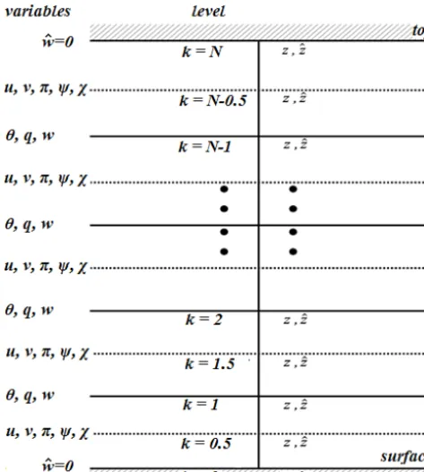
X=(u,v, m, q)T, (1) whereuand v are the wind components, q is the specific humidity, andmdenotes the mass field of the Exner pres-sureπ. Although GRAPES is a non-hydrostatic model, we do not consider the non-hydrostatic property of GRAPES-Var system currently. The Exner pressureπ is chosen as the state vector and the potential temperature θ is the deriva-tion ofπ. We also do not consider the analysis of the hy-drometeors. Figure 1 shows the schematic of the atmospheric status and analysis variables of GRAPES-Var in the Char-ney–Phillips vertical grid. The GRAPES model top is ap-proximately 32 km, with 36 vertical layers. The design of the RO observation operator is required to meet such grid and variable definition to exert its maximal assimilation impact.
Figure 1. Schematic diagram of the atmospheric status and analy-sis variables of GRAPES-Var in the Charney–Phillips vertical grid (from Xue et al., 2012).
sea surface wind, radar observation, and so on. The satel-lite radiance observations used in GRAPES are mainly Ad-vanced Microwave Sounding Unit-A (AMSU-A) from the polar satellites and the AIRS hyperspectral infrared obser-vation. The assimilation window is 6 h.
3 Assimilation of the RO data
3.1 Choice of observation to assimilate
The RO measurements undergo different data processing stages when moving from the raw data of phase and am-plitude, to bending angle, to refractivity to the retrieval of the temperature and water vapour pressure, any of which can be assimilated. Generally, it is better to assimilate rawer observations because the observation error is relatively sim-ple; however, the assimilation of rawer data results in a more complex observation operator and more expensive computer cost. The favourite RO measurements assimilated in an op-erational NWP system are ionosphere-corrected bending an-gles and refractivity (Eyre, 1994; Kuo et al., 2000).
At an early stage, GRAPES assimilated the water vapour and temperature data derived from radio occultation obser-vations (see Sect. 3.5.1). The advantage of this approach is that the data are in a form similar to the model variables and can be readily used. However, these assimilated data are the highest level retrievals and due to longer path contain the
most approximation errors. The accuracies of the retrievals are strongly affected by the accuracy of the ancillary data, thus resulting in a correlation between the background and observation error in assimilation. The propagation of the ob-servation error is more complex when using the retrievals.
The precision of the refractivity is higher than that of the retrieved temperature and water vapour, and its observa-tion operator is simpler. Therefore, assimilating refractivity is better than assimilating temperature and water vapour. The bending angle is a rawer product compared to refractivity; however, the bending angle operator must integrate the bend-ing from the tangent point upward; these integrals will be in-accurate if the tangent height is near the model top (Aparicio and Deblonde, 2008). In particular, if the model top is not sufficiently high (above 60 km), the modelling error of the bending angle will be relatively large, whereas the height of the model top does not affect the calculation of refractivity (Rennie, 2010). The model top of GRAPES is only 32.5 km; therefore, we assimilate the refractivity rather than the bend-ing angle. But the retrieval from the bendbend-ing angle to the refractivity uses the assumption of local spherical symme-try, the presence of horizontal gradients limits the accuracy (Sokolovskiy et al., 2005; Healy et al., 2007). To obtain more proper information from the RO data, a non-local refractivity or a ray-tracing observation operator is more appropriate. 3.2 Pre-processing
3.2.1 Conversion of coordinates
Refractivity is reported as a function of geometric altitude by the data processing centres. In the RO data pre-processing system, we first convert the vertical coordinate of the RO data from geometric altitude to geopotential height, which is the coordinate of GRAPES. The geopotential heightH is calcu-lated based on the World Geodetic System 1984 (WGS-84) World Geodetic Model (NIMA, 2004) ellipsoid parameters:
H= 1
g0 z
Z
0
gWGS84(ϕ, z)dz, (2)
whereg0=9.80665 m s−2 is the standard gravitational ac-celeration that is defined at sea level and 45◦latitude, and
gWGS84(ϕ, z)is the approximation of the actual gravitational acceleration as a function of latitudeϕ and geometric alti-tudez.
3.2.2 Quality control
five times the bi-weight standard deviation based on the high (60–90◦N/S), medium (30–60◦N/S) and low (30◦S–30◦N)
latitudinal belt at each vertical level. This step removes rela-tively few data, primarily near the surface, because the qual-ity of the RO data is good.
The second QC procedure is to remove the RO data that possibly exhibit super refractions. The RO technique relies on the propagation of L-band radio waves within the Earth’s atmosphere. Super refraction occurs when the vertical re-fractivity gradient exceeds the critical refraction, resulting in negative refractivity bias after an Abel transform inversion (Rocken et al., 1997). Software improvement had failed to solve this error (Sokolovskiy, 2003). Therefore, by follow-ing the method proposed by Poli et al. (2009), suspicious observations located below regions where dN/dzfalls be-low −50 N km−1 and
d2N/d2z
exceeds 100 N2km−2 are
sequentially flagged.
Finally, a background check is performed. If the innova-tion vector (the difference between the observainnova-tion and fore-cast field) exceeds a certain threshold (namely,|No−Nb|>
ασo), then the observation is rejected. In this case, the ratio
αis four times the observation error standard deviation. The background check rejects approximately 10 % of the refrac-tivity data.
3.2.3 Thinning
The vertical sampling of the refractivity profile is thinned 100 to 300 m from the near surface to approximately 60 km, de-pending on the data processing centre. The vertical resolution is much higher than that of the GRAPES model. To avoid high correlation between observation errors and keep suffi-ciently fine observation information, we only use the obser-vations nearest each vertical analysis level in the RO profiles. 3.3 Observation operator
In a variational data assimilation system, the analysis of the atmospheric state x must be found by minimizing the cost function
J (x)=1 2(x−xb)
TB−1(x−x b)+
1
2(H (x)−y)
TR−1(H (x)−y),
(3) wherexbis the background field (e.g. a short-term forecast), y is a vector of observations, B and R are the covariance matrices of background and observation error, respectively, andH (x) is the observation operator, which calculates the observation using the statex. To obtain the optimal analysis in Eq. (3), the gradient ofJ
∇xJ (x)=B−1(x−xb)+HTR−1(H(x−xb)+d) (4) must be calculated, where H is a linear approximation of the observation operatorH (x)in the vicinity ofxb, anddis the
innovation vectord=yo−H (xb). The final analysis is the optimal fit between the observation and the background.
In GRAPES-Var, the RO operator is refractivity, which is expressed as
N=77.6·P
T +3.73·10
5· e
T2, (5)
whereN is the refractivity in N-unit, P is the pressure in hPa,T is the temperature in Kelvin, andeis the water vapour pressure in hPa. The atmospheric state variables at GRAPES are Exner pressure, specific humidity, and wind components (uandv) rather than pressure, temperature and water vapour pressure. Therefore, the calculation ofH (x)in Eqs. (3) and (4) will use following relationships:
π=
P
P0
Rd/CP
(6)
p=p0π CP
Rd (7)
T =π θ (8)
q=0.622· e
P −0.378·e, (9)
whereCP=1004.5 Jkg−1K−1 is the specific heat capacity of dry air at constant pressure,Rd=287.05 Jkg−1K−1is the specific gas constant for dry air and P0=1000 hPa is the reference surface pressure. The corresponding tangent linear operators are
δp=p0CP
R π
CV
Rdδπ (10)
δT =θ δπ+CPπ θ 2 g ∂δπ ∂z (11) As a result of using the Charney–Phillips staggering grid, the pressure, temperature and specific humidity are not in the same vertical level. Based on Fig. 1, the background refrac-tivity is defined at theθ level like that of the Met. Office (Rennie, 2008). The error induced by variable transformation and vertical interpolation is reduced because we only inter-polateπ; otherwise we must interpolateθ andq.π at theθ
level is calculated by assuming a linear variation ofπ with geopotential height:
πk=
(zk−zk−1/2) (zk+1/2−zk−1/2)
πk+1/2+
(zk+1/2−zk) (zk+1/2−zk−1/2)
πk−1/2. (12)
Then, the pressure at the θ level is obtained based on Eq. (7).
The mean virtual temperature at theθ level is calculated using the hydrostatic equation:
Tk=πkθk= − 1
(1+bqk)
g CP
(zk+1/2−zk−1/2)
(lnπk+1/2−lnπk−1/2)
, (13)
whereg=9.80665 m s−2 is the mean gravity acceleration,
Figure 2. Geopotential height comparisons between the GRAPES and NCEP analyses. (a) is the 500 mb correlation coefficient in the NH; (b) is the 500 mb RMSE (GRAPES minus NCEP) in the NH; (c) is the same as (a), except it is for the SH instead of the NH; (d) is the same as (b), except it is for the SH instead of the NH. In (a–d), the black, blue and red lines correspond to the experiments performed in 2007, 2008 and 2009, respectively; (e–f) are the latitude–pressure plots of the annual mean difference (GRAPES minus NCEP) for the experiments in 2007 and 2009, respectively.
The background refractivity profiles at the four grid points nearest the occultation latitude and longitude are calculated first. Next, the background refractivity profile at the occulta-tion locaocculta-tion is obtained using bi-linear interpolaocculta-tion. Finally, the linear interpolation of log-N is applied in the vertical di-rection to get the background refractivity at the occultation observation location. The drift of the tangential point is not taken into account.
The RO observation error standard deviationσois obtained using the following formula:
σo=
σ
100·N, (14)
whereσ is the normalized observation error standard devi-ation, which is a function of latitude and height (Liu and Xue, 2014). We firstly refer to the refractivity error of the Met. Office (Rennie, 2010), then use one-month results and the method proposed by Desroziers et al. (2005) to evaluate
analysis, background and observation error covariance matri-ces in observation space, and tune the specified observation error used in the data assimilation system.
Figure 3. Mean (dashed line) and RMSE (solid line) between the background (grey) and analysis (black) to the refractivity as a func-tion of geopotential height, which is normalized using observafunc-tion error. The grey line indicates the background minus observation, and the black line indicates analysis minus observation. The lefty -axis denotes the height, and the righty-axis denotes the RO number assimilated in each level. Experiment period is from 00:00 UTC on 1 July to 18:00 UTC on 31 July 2011 (from Liu and Xue, 2014).
3.4 Assimilation and forecast impact experiments 3.4.1 Early pre-operational trials
Before presenting the effect of RO data on GRAPES, we briefly review the early pre-operational trials. The original experimental system of the GRAPES data assimilation and forecast model with regional and global configurations was set up in 2005 (Xue, 2006; Xue et al., 2008; Chen et al., 2008). Since 2007, 1-year period global pre-operational tri-als have been conducted to evaluate the model performance every year. GRAPES-Var could only assimilate conventional observations (radiosonde, synop, ships, aircraft and cloud drift wind) and satellite radiance (AMSU-A from NOAA-16 and -18) at that time. Figure 2 shows the performance of GRAPES-Var, including correlation coefficients at 500 hPa, the root mean square error (RMSE) in 500 hPa and the mean difference for geopotential height from 1000 to 10 hPa, com-pared to the NCEP analyses. Note that often, even now, we use ECMWF and NCEP analyses (reanalyses) to evaluate the model performance, because GRAPES is a developing sys-tem and the types of observations assimilated in GRAPES-Var are still limited, whereas the analyses from advanced NWP centres include a large amount of information from satellite remote sensing data; as a result, it is easier to iden-tify the problems of GRAPES when the simulations are com-pared with these analyses. GRAPES-Var is found to have
two distinct issues in the early version. The first one is that GRAPES exhibits significant biases in the polar, equatorial and upper regions. The second one is that the bias of the SH in winter increases suddenly. Most problems occur in the SH, which indicates that these problems are mainly related to the lack of observations and to model error. Therefore, more ob-servations should be assimilated into the GRAPES system to reduce the bias.
Of the three trials presented in Fig. 2, only the 2009 trial assimilates RO data. After assimilating the RO data, the dif-ferences with the NCEP analyses in the SH and the strato-sphere are greatly reduced, and the explosive growth bias of the SH during winter time is also solved. Although other improvements in the data assimilation system and forecast model are integrated in the 2009 trial, the greatest contribu-tion is from the RO data. Notably, in this trial, we assimilate the COSMIC retrieval temperature and water vapour data. These retrieval profiles are based on 1-D variational analysis using ECMWF analysis data, and collocated with occulta-tion profiles. The retrievals of temperature and water vapour exhibit the greatest approximation error, and their observa-tion errors might be correlated with background error; but they still have a significant impact on data assimilation when only a few observations are assimilated, especially in the SH. Since the 2009 trial, we have updated the RO observation op-erator from the retrievals to the refractivity at GRAPES-Var. 3.4.2 Recent observation impact experiments
As mentioned in Sect. 3.1, GRAPES-Var has been updated from the early pressure-based to the height-based (Xue et al., 2012). Accordingly, the expression of refractivity oper-ator changes, and the impact of RO in the new data assimila-tion system has to be re-evaluated. In the observaassimila-tion impact experiment, we employ a relatively simple control experi-ment in which only the conventional observations are assim-ilated. We then assimilate the RO data on the basis of the control experiment. The aim is to observe the effect of the RO data more clearly. The experimental period is 1 month, from 00:00 UTC 1 July to 18:00 UTC 31 July 2011, and the RO data include COSMIC and METOP-A/GRAS data.
Figure 4. Analysis comparisons between the control and RO experiment for temperature (first row), specific humidity (second row), and zonal wind (third row). The first column shows the monthly mean difference between the control experiment and NCEP analysis (control minus NCEP). The second column shows the monthly mean difference between the RO experiment and NCEP analysis (RO minus NCEP). The contour intervals in the three rows are 0.5 K, 0.2 kg kg−1×10+3and 0.5 m s−1respectively. Experiment period is from 00:00 UTC on 1 July to 18:00 UTC on 31 July 2011.
Figure 4 presents comparisons between GRAPES and NCEP analysis. The temperature difference between the con-trol experiment and the NCEP analysis is mainly found in the SH and near the tropical tropopause. The biases are clearly reduced after assimilating the RO observations. The number of conventional observations in the SH are about 5 % of the same latitude zone in the NH. As a result, once the occulta-tion observaocculta-tions are assimilated, a significant improvement in the analysis can be seen. The improvement of humidity field after assimilation of RO observations is a little bit better in most areas, except for the middle and lower troposphere in the low latitudes of SH. The cause is under investigation.
For the zonal wind analysis, the differences with and with-out the RO data are concentrated in the tropics as well as in the Southern Hemisphere. But the improvement of RO ob-servation assimilation on wind analysis in the tropics is not as obvious as in the SH. This illustrates that the relationship between pressure and wind field is in geostrophic balance in
the middle and high latitudes – the analysis of wind is nat-urally improved by the adjustment of mass field. However, the coupling between wind and pressure field is very weak in the tropical region – an observation providing information on the mass will not work on the dynamical analysis even with further increases in occultation observations. The fur-ther improvements of wind analysis in the tropical regions rely on more wind observations being available, the reduc-tion of model bias and the assimilareduc-tion scheme.
Figure 5. Anomaly correlation coefficient (ACC) for the 500 mb height for the 8-day forecast. The dashed line denotes the con-trol experiment only assimilating conventional observation, and the solid line denotes the RO assimilation experiment. The black lines denote the Northern Hemisphere, the red lines denote the Southern Hemisphere, and the green lines denote the East Asia. Experiment period is from 12:00 UTC on 1 July to 12:00 UTC on 31 July 2011; it is from 31 samples (from Liu and Xue, 2014).
contrast of the RO and control experiments in the NH is not as obvious as that in the SH because of the high density of radiosonde observations in the NH. The ACC of the RO periment is even slightly lower than that of the control ex-periment in East Asia in 96 h. Overall, RO observations have positive impacts at any range and in any area.
The above results are based on a 1-month period experi-ment; for more details, see Liu and Xue (2014).
3.4.3 Full observation impact experiments
Figures 6 and 7 are the results of RO data in the full obser-vation impact experiments. The experiment period is from 06:00 UTC 1 May to 18:00 UTC 31 May 2013. The assim-ilation window is 6 h. We have done two experiments. One is a control run (all observations run), and the other is the RO run. In the control experiment we assimilate conventional observations (radiosonde, synop, ships, aircraft, cloud drift wind), RO (COSMIC, METOP-A & B, GRACE-A), AMSU-A (NOAMSU-AAMSU-A-15,16,18,19 and Metop-AMSU-A) and AMSU-AIRS hyperspec-tral infrared observation, which is the current configuration of operational GRAPES-VAR. In the RO experiment we take out the RO data from the full observation assimilation. Fig-ure 6 presents the comparisons of the RMSE of the temper-ature and zonal wind between the GRAPES analysis and the ERA-Interim reanalysis (Dee et al., 2011) in the NH, SH and tropical areas. No matter in which area, the RO data have positive impact on the analysis; the impact in the SH, tropi-cal areas and upper levels are more prominent. Figure 7 is the anomaly correlation coefficient for the 500 mb height calcu-lated for the full observations and no-RO data experiment
Figure 6. RMSE of temperature (a) and zonal wind (b) analysis between full observations and no RO data assimilation experiments, compared to EC-Interim reanalysis (GRAPES minus EC-Interim) in the Southern Hemisphere for the full observations (solid line) and the no-RO data (dashed line) experiments. Black, red and blue lines are the RMSE in NH, SH and tropical areas, which are the monthly average RMSE from 06:00 UTC 1 May to 18:00 UTC 31 May 2013.
8-day forecast as a function of time. The impact of RO data on forecast is evident, especially in the SH.
3.5 A long-term RO experiment
with-Figure 7. Anomaly correlation coefficient (ACC) for the 500 mb height for the 8-day forecast. The solid line denotes the full ob-servations experiment, and the dashed line denotes the experiment without RO observation. The black lines denote the Northern Hemi-sphere, the red lines denote the Southern Hemisphere. Experiment period is same to that of Fig. 6; it is from 31 samples.
Figure 8. RMSE of geopotential height analysis between GRAPES and NCEP (GRAPES minus NCEP) in the Southern Hemisphere for the control (dashed line) and the RO (solid line) experiment. Green, red and blue lines are the RMSE in the initial time, 15th and 30th day, respectively; the black lines are the monthly average RMSE.
out drift compared with NCEP analysis, even after 9 months. It is well known that the largest effect of satellite observa-tions on NWP is in the SH, where conventional observaobserva-tions are sparse. Figure 8 also demonstrates this point by showing a comparison of the RMSE of the geopotential height be-tween the GRAPES and the NCEP analysis in the SH as a function of time for the control and the RO experiment. In these two experiments, the RMSE is relatively fixed under
Figure 9. Mean (dashed line) and RMSE (solid line) of the 50 hPa temperature analysis difference between GRAPES and NCEP (GRAPES minus NCEP) in a cycle running from 00:00 UTC 1 July 2011 to 18:00 UTC 16 April 2012. Black lines denote the results of the NH, and red lines denote the results of the SH.
100 hPa because most conventional observations (e.g. cloud drift wind, synoptic and ships observation) are limited in the lower troposphere. However, the RMSE of the control ex-periment increases with time above 100 hPa; for example, at 10 hPa, the RMSE of geopotential height increases 10 times from 30 geopotential metres at the initial time to 300 geopo-tential metres on the 30th day. Once the RO data are assim-ilated, the RMSE from the surface to the model top seldom changes with time.
As an example, Fig. 9 presents the evolution of the mean temperature bias and the RMSE between the GRAPES and NCEP analysis in the RO experiment at 50 hPa for both spheres. The difference of RMSE values between each hemi-sphere gradually decreases with height (figure omitted). This result illustrates that the number and distribution of the ob-servations are important factors that affect the analysis per-formance of the data assimilation system. The number of ra-diosondes station is greater in the NH than in the SH, and more observations are in the troposphere, whereas the RO ob-servations gradually dominate in the upper troposphere and stratosphere for both hemispheres. Therefore, the differences with the NCEP analysis between the NH and the SH gradu-ally decreases with height.
4 Simulation of FY-3 RO events
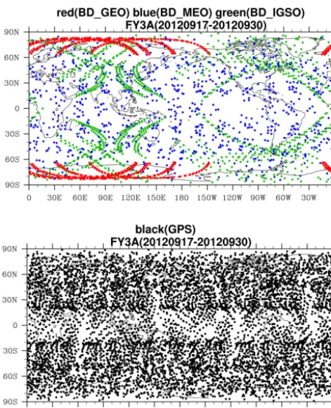
FY-Figure 10. Beidou (top) and GPS (bottom) occultation events sim-ulation based on FY-3A satellite orbit parameters. Red dots denote the RO of the Beidou geostationary satellites, blue dots denote the RO of the Beidou middle-orbit satellites, and green dots denote the RO of the Beidou inclined geosynchronous satellites. The simula-tion period is from 17 to 30 September 2012.
3C satellite has launched, and real GPS and Beidou RO data have been obtained (Bai et al., 2014), which comprise more than 500 RO events daily, including approximately 400 GPS and 100 Beidou RO events; the relevant results will be pre-sented in another special paper – therefore, only the simu-lated occultation events of the Beidou and the GPS satellite with the present Beidou and FY-3A satellite orbit parameters are shown here (Fig. 10). Currently, 14 Beidou operational satellites are in orbit, including five geostationary satellites, five inclined geosynchronous satellites and four middle-orbit satellites. The orbits of Beidou navigation satellite differ from those of the GPS, GLONASS and Galileo navigation satellite systems. More RO events are observed in the polar regions than before, due to the five geostationary satellites of the Beidou system.
5 Summary and further work
The above results demonstrate that the assimilation of RO data provides useful information for GRAPES and has a clearly positive impact on the analysis and forecasts at all ranges, confirming the findings of other operational NWP
centres. Although most of these results are based on a rel-atively simple experimental system or a simple baseline ex-periment, which might amplify the effect of the RO data, they easily distinguish the contribution of the RO data.
The RO technique produces highly accurate observations with a uniform global distribution and very high vertical res-olution in the upper atmosphere, where the model errors are large. Furthermore, RO observations do not require bias cor-rection. Therefore, even a simple data assimilation system in which only conventional and RO data are assimilated can run stably for a long time, and still have analysis and forecast performance. Ultimately, the real impact of RO needs tun-ing in a full observations operational system in which a great amount satellite data are assimilated. RO data have coarse horizontal resolution, but radiance observations “anchored” by GNSS-RO can indirectly spread the information with bet-ter horizontal resolution in a full observation system. They complement each other.
The development of RO data assimilation in GRAPES-VAR has experienced three stages since 2008: the assimi-lation of retrieval products in a pressure-based coordinate data assimilation system, the assimilation of refractivity in a pressure-based coordinate version, and the assimilation of refractivity in a height-based coordinate version. The vari-able assimilated, the definition of coordinate and analysis variables of an assimilation system are different, resulting in the difference of the observation operation expression. But, whatever variable we assimilate, or whatever data assimi-lation system we use, the RO data have positive effects on analysis and forecast in GRAPES. Besides the advantages of RO observations themselves, another important reason is that the observation types and amount assimilated in GRAPES are still limited, resulting in the predominant effect of RO in GRAPES-VAR.
Currently, GRAPES assimilates refractivity due to its lower model top of only 32.5 km. The assimilation of the bending angle provides a larger positive effect on the fore-cast accuracy compared to the refractivity when the model top is high. Therefore, we need to develop the bending angle observation operator when the global model top is raised. We also take into account the effect from the spherical symmetry assumption, and develop the non-local observation operators. In addition, we shall take into account the vertical correlation of observation error.
RO has become one important part of the global observing system. However, the quantity of RO is decreasing due to the aging of the COSMIC satellites. New RO missions should be supplemented urgently. To gain more RO observation, there is a requirement to place more emphasis on the new RO ob-servation usage, such as FY-3C/GNOS RO data.
(GYHY201106008 and GYHY201206007). The authors thank Zhuang Zhaorong for providing Fig. 2.
Edited by: A. von Engeln
References
Anthes, R. A.: Exploring Earth’s atmosphere with radio occulta-tion: contributions to weather, climate and space weather, At-mos. Meas. Tech., 4, 1077–1103, doi:10.5194/amt-4-1077-2011, 2011.
Anthes, R. A., Bernhardt, P. A., Chen, Y., Cucurull, L., Dymond, K. F., Ector, D., Healy, S. B., Ho, S. P., Hunt, D. C., Kuo, Y.-H., Liu, H., Manning, K., McCormick, C., Meehan, T. K., Randel, W. J., Rocken, C., Schreiner,W. S., Sokolovskiy, S.V., Syndergaard, S.,Thompson, D. C., Trenberth, K. E., Wee, T. K., Yen, N. L., and Zeng, Z.: The COSMIC/FORMOSAT-3 Mission-Early results, B. Am. Meteorol. Soc., 89, 313–333, 2008.
Aparicio, J. M. and Deblonde, G.: Impact of the assimilation of CHAMP refractivity profiles on Environment Canada global forecasts, Mon. Weather Rev., 136, 257–275, 2008.
Bai, W. H., Sun, Y. Q., Du, Q. F., Yang, G. L., Yang, Z. D., Zhang, P., Bi, Y. M., Wang, X. Y., Cheng, C., and Han, Y.: An introduc-tion to the FY3 GNOS instrument and mountain-top tests, At-mos. Meas. Tech., 7, 1817–1823, doi:10.5194/amt-7-1817-2014, 2014.
Buontempo, C., Jupp, A., and Rennie, M. P.: Operational NWP as-similation of GPS radio occultation data, Atmos. Sci. Lett., 9, 129–133, 2008.
Chen, D. H., Xue, J. S., Yang, X. S., Zhang, H.-L., Shen, X.-S., Hu, J.-L., Wang, Y., Ji, L.-R., and Chen J.-B.: New generation of multi-scale NWP system: general scientific design, Chinese Sci. Bull., 53, 3433–3445, 2008.
Collard, A. D. and Healy, S. B.: The combined impact of fu-ture space-based atmospheric sounding instruments on numeri-cal weather prediction analysis fields: a simulation study, Q. J. Roy. Meteor. Soc., 129, 2741–2760, 2003.
Cucurull, L., Derber, J., Treadon, R., and Purser, R. J.: Assimilation of global positioning system radio occultation observations into NCEP’s global data assimilation system, Mon. Weather Rev., 135, 3174–3193, 2006.
Dee, D. P., Uppala, S. M., Simmons, A. J., Berrisford, P., Poli, P., Kobayashi, S., Andrae, U., Balmaseda, M. A., Balsamo, G., Bauer, P., Bechtold, P., Beljaars, A. C. M., van de Berg, L., Bid-lot, J., Bormann, N., Delsol, C., Dragani, R., Fuentes, M., Geer, A. J., Haimberger, L., Healy, S. B., Hersbach, H., Hólm, E. V., Isaksen, L., Kållberg, P., Köhler, M., Matricardi, M., McNally, A. P., Monge-Sanz, B. M., Morcrette, J. J., Park, B. K., Peubey, C., de Rosnay, P., Tavolato, C., Thépaut, J.-N., and Vitart, F.: The ERA-Interim reanalysis: configuration and performance of the data assimilation system, Q. J. Roy. Meteor. Soc., 137, 553–597, doi:10.1002/qj.828, 2011.
Desroziers, G., Berre, L., Chapnik, B., and Poli, P.: Diagnosis of ob-servation, background and analysis-error statistics in observation space, Q. J. Roy. Meteor. Soc., 131, 3385–3396, 2005.
Eyre, J. R.: Assimilation of radio occultation measurements into a numerical weather prediction system, Technical Memo. No. 199, ECMWF, Reading, UK, 1994.
Fjeldbo, G. and Eshleman, V. R.: The atmosphere of Mars analysed by integral inversion of the Mariner IV occultation data, Planet Space Sci., 16, 1035–1059, 1968.
Healy, S. B.: Forecast impact experiment with a constellation of GPS radio occultation receivers, Atmos. Sci. Lett., 9, 111–118, 2008.
Healy, S. B., Jupp, A. and Marquardt, C.: Forecast impact experi-ment with GPS radio occultation measureexperi-ments, Geophys. Res. Lett., 32, L03804, doi:10.1029/2004GL020806, 2005.
Healy, S. B., Eyre, J. R., Hamrud, M., and Thepaut, J.-N.: Assimilat-ing GPS radio occultation measurements with two-dimensional bending angle observation operators, Q. J. Roy. Meteor. Soc., 133, 1213–1227, doi:10.1002/qj.63, 2007.
Kuo, Y.-H., Sokolovskiy, S., Anthes, R. A., and Vandenberghe, F.: Assimilation of GPS radio occultation data for numerical weather prediction, Atmos. Ocean. Sci., 11, 157–186, 2000. Kursinski, E. R., Hajj, G. A., Schofield, T., Linfield, R. P., and
Hardy, K. R.: Observing Earth’s atmosphere with radio occulta-tion measurements using the global posiocculta-tioning system, J. Geo-phys. Res., 102, 23429–23465, doi:10.1029/97JD01569, 1997. Lanzante, J. R.: Resistant, robust and nonparametric techniques for
the analysis of climate data: theory and examples, Int. J. Climate, 16, 1197–1226, 1996.
Liu, Y. and Xue, J.-S.: Assimilation of global navigation satellite radio occultation observations with GRAPES: Operational im-plementation, J. Meteor. Res., 28, in press, doi:10.1007/s13351-014-4028-0, 2014.
NIMA: Department of defense World Geodetic System 1984: its definition and relationships with local geodetic system, National Geospatial Intelligence Agency Tech. Rep. TR8350.2, 175 pp., National imagery and mapping agency, USA, 2004.
Poli, P.: 1DVAR analysis of temperature and humidity using GPS radio occultation refractivity data, J. Geophys. Res., 107, 4448, doi:10.10.1029/2001JD000935, 2002.
Poli, P., Moll, P., Puech, D., Rabier, F., and Healy, S. B.: Quality control, error analysis, and impact assessment of FORMOSAT-3/COSMIC in numerical weather prediction, Terr. Atmos. Ocean. Sci., 20, 101–113, 2009.
Rennie, M. P.: The Assimilationof GPS Radio Occultation data into the Met Office global model, http://www.metoffice.gov.uk/ archive/forecasting-research-technical-report-510 (last access: 22 November 2014), 2008.
Rennie, M. P.: The impact of GPS radio occultation assimilation at the Met Office, Q. J. Roy. Meteor. Soc., 136, 116–131, 2010. Rocken, C., Anthes, R., Exner, M., Hunt, D., Sokolovskiy, S., Ware,
R., Gorbunov, M., Schreiner, W., Feng, D., Herman, B., Kuo, Y.-H., and Zou, X.: Analysis and validation of GPS/MET data in the neutral atmosphere, J. Geophys. Res., 102, 29849–29866, doi:10.1029/97JD02400, 1997.
Ware, R., Rocken, C., Solheim, F., Exner, M., Schreiner, W., An-thes, R., Feng, D., Herman, B., Gorbunov, M., Sokolovskiy, S., Hardy, K., Kuo, Y., Zou, X., Trenberth, K., Mee-han, T., Melbourne, W., and Businger, S.: GPS sounding of the atmosphere from low earth orbit: Preliminary re-sults, B. Am. Meteorol. Soc., 77, 19–40, doi:10.1175/1520-0477(1996)077<0019:GSOTAF>2.0.CO:2, 1996.
Sokolovskiy, S, Kuo, Y. H, and Wang, W. E.: valuation of a linear phase observation operator with CHAMP radio occulation data and high-resolution regional analysis, Mon. Weather Rev., 2005, 133, 3053–3059, 2005.
Xue, J.-S.: Progresses of researches on numerical weather predic-tion in China: 1999–2002, Adv. Atmos. Sci., 21, 467–474, 2004. Xue, J.-S.: Progress of Chinese numerical prediction in the early new century, J. Appl. Meteorol. Sci., 17, 602–610, 2006 (in Chi-nese).
Xue, J.-S. and Chen, D.-H.: Scientific design and application of GRAPES, Science Press, Beijing, 1–383, 2008 (in Chinese). Xue, J.-S., Zhuang, S.-Y., Zhu, G.-F., Zhang, H., Liu, Z.-Q., Liu,
Y., and Zhuang, Z.-R.: Scientific design and preliminary re-sults of three dimensional variational data assimilation system of GRAPES, Chinese Sci. Bull., 53, 3446–3457, 2008.
Xue, J.-S., Liu, Y., and Zhang, L.: Scientific documentation of GRAPES-3DVar version for the global model, Numerical Weather Prediction Center, China Meteorological Administra-tion, 2012 (in Chinese).
Yunck, T. P.: An overview of atmospheric radio occultation, Journal of Global Positioning System, 1, 58–60, 2002.