R E S E A R C H
Open Access
Temporal variation of ecosystem carbon
pools along altitudinal gradient and slope:
the case of Chilimo dry afromontane
natural forest, Central Highlands of Ethiopia
Mehari A. Tesfaye
1*, Oliver Gardi
2, Tesfaye Bekele
1and Jürgen Blaser
2Abstract
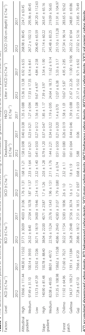
Quantifying the amount of carbon pools in forest ecosystems enables to understand about various carbon pools in the forest ecosystem. Therefore, this study was conducted in the Chilimo dry afromontane forest to estimate the amount of carbon stored. The natural forest was stratified into three forest patches based on species composition, diversity, and structure. A total of 50 permanent sample plots of 20 m × 20 m (400 m2) each were established, laid out on transects of altitudinal gradients with a distance of 100 m between plots. The plots were measured twice in 2012 and 2017. Tree, deadwood, mineral soil, forest floor, and stump data were collected in the main plots, while shrubs, saplings, herbaceous plants, and seedling data were sampled inside subplots. Soil organic carbon (SOC %) was analyzed following Walkely, while Black’s procedure and bulk density were estimated following the procedure of Blake (Methods of soil analysis, 1965). Aboveground biomass was calculated using the equation of Chave et al. (Glob Chang Biol_20:3177–3190, 2014). Data analysis was made using RStudio software. To analyze equality of means, we used ANOVA for multiple comparisons among elevation classes atα= 0.05. The aboveground carbon of the natural forest ranged from 148.30 ± 115.02 for high altitude to 100.14 ± 39.93 for middle altitude, was highest at 151.35 ± 108.98 t C ha−1for gentle slope, and was lowest at 88.01 ± 49.72 t C ha−1for middle slope. The mean stump carbon density 2.33 ± 1.64 t C ha−1was the highest for the middle slope, and 1.68 ± 1.21 t C ha−1was the lowest for the steep slope range. The highest 1.44 ± 2.21 t C ha−1deadwood carbon density was found under the middle slope range, and the lowest 0.21 ± 0.20 t C ha−1was found under the lowest slope range. The SOCD up to 1 m depth was highest at 295.96 ± 80.45 t C ha−1 under the middle altitudinal gradient; however, it was lowest at 206.40 ± 65.59 t C ha−1 under the lower altitudinal gradient. The mean ecosystem carbon stock density of the sampled plots in natural forests ranged from 221.89 to 819.44 t C ha−1. There was a temporal variation in carbon pools along environmental and social factors. The highest carbon pool was contributed by SOC. We recommend forest carbon-related awareness creation for local people, and promotion of the local knowledge can be regarded as a possible option for sustainable forest management.
Keywords: Carbon stock density, Dry afromontane natural forest, Deadwood, Humus, Herbaceous, Mineral soil and stump carbon
© The Author(s). 2019Open AccessThis article is distributed under the terms of the Creative Commons Attribution 4.0 International License (http://creativecommons.org/licenses/by/4.0/), which permits unrestricted use, distribution, and reproduction in any medium, provided you give appropriate credit to the original author(s) and the source, provide a link to the Creative Commons license, and indicate if changes were made. The Creative Commons Public Domain Dedication waiver (http://creativecommons.org/publicdomain/zero/1.0/) applies to the data made available in this article, unless otherwise stated. * Correspondence:meharialebachew25@gmail.com
1Ethiopian Environment and Forest Research Institute (EEFRI), Box 24536 code 1000, Gurd Shola, Addis Ababa, Ethiopia
Background
Forest provides goods, such as wood and non-wood for-est products (NWFP), and ecosystem services, such as biodiversity protection, fresh water supply, soil protec-tion, and climate regulaprotec-tion, which are important for the well-being of the people at local, national, and global
levels. Forests mitigate atmospheric CO2 as sinks in its
carbon pools (C sequestration). IPCC (2013) reported
that the global forest cover is 4 billion hectares and rep-resents over 50% of global greenhouse gas mitigation
po-tential (IPCC 2007). Tropical, humid, and dry forests
spread over 2.1 billion hectare area worldwide, store 180 Gt C stock in biomass, and have a turnover of 915 Gt of carbon each year (Millennium Ecosystem
Assess-ments2005; Baccini et al.2008; FRA 2015). Tropical dry
forests cover over 840,000,000 ha, constitute a net terres-trial primary production of 40% of all tropical forests,
and store 60% carbon which contain half of the world’s
tree species (Miles et al.2006; Chidumayo et al.2011).
The major carbon pools in forest ecosystems are aboveground and belowground biomass, deadwood,
lit-ter, and soil organic carbon (FAO 2005; IPCC 2003,
2006). Aboveground biomass (AGB) includes all living
biomass above the soil, while belowground biomass (BGB) includes all biomass of live roots excluding fine
roots (< 2 mm diameter) (Brown 1997; IPCC 2003).
Deadwood organic carbon includes coarse and fine deadwood found in the form of logged, standing and
lying deadwood (Takahashi et al. 2010; Kassa 2015).
Litter carbon is found in the form of fallen leaves, twigs,
and undecomposed litter (Lemma et al. 2007). The soil
is the largest carbon reservoir of the terrestrial carbon
cycle storing 1500–1550 Gt of organic carbon. About
three times more carbon is contained in soils than in the
world’s vegetation 560 Gt, and soils hold more than
twice the amount of carbon, i.e., present in the
atmos-phere 720 Gt (Post et al. 2001; Lal 2004). Forest soil is
part of any forest ecosystem and stores about 40% of the
total SOC of the global soils (Baker2007; Rooney 2013).
The carbon pools in forest ecosystems are affected by
altitude, slope, and land-use types (Diawei et al. 2006).
Bhat et al. (2013) indicated that land use, land-use
changes, soil erosion, and deforestation are the most im-portant factors affecting the carbon stock density in the forest ecosystem. According to Feyissa et al. (2013), for-est carbon is affected by altitude and slope. Altitude has a significant effect on temperature and precipitation. This strongly affects the species composition, the diver-sity, the quantity, and the turnover of forest ecosystem
(Sheikh and Bussmann 2009). Hamere et al. (2015)
assessed the impact of slope in above and belowground biomass, soil organic carbon, and total ecosystem car-bon, in which east slope aspect showed the highest, whereas south slope aspect showed the lowest total
carbon stock. In the tropics, land use affects the global carbon cycle by increasing the rate of carbon emissions
(Silver et al. 2000). Conversion of forest land use type
into agricultural land use types reduced SOC stock
density by 20–50% (Solomon et al. 2002; Lemenih
and Itanna 2004; Lal2005).
Ethiopia is endowed with various landscape types. Ac-cordingly, the vegetation types are diverse and vary from tropical humid forests and cloud forests located in the southwest to desert scrubs in the east and northeast
(Bongers and Tenngkeit 2010). The natural high forests
of Ethiopia are mainly found in the highlands where an-nual rainfall distribution and amount is better, with a maximum mean annual rainfall of more than 1000 mm
year−1. Around 90% of the total population live in the
highlands, which covers 44% of the country’s land mass.
Moreover, the great majority (93%) of the cultivated land
and the country’s livestock population (75%) is found in
the highlands.
The national carbon stock of Ethiopia was estimated
to be 153 teragram (Tg) of C by Houghton (1998), 867
Tg of C by Gibbs et al. (2007), and 2.5 Gt of C by Sisay
(2010). The natural high forest carbon stock ranges from
101 to 200 Mg C ha−1 (Brown 1997; Moges et al. 2010;
Temam 2010; Tsegaye 2010). The discrepancy between
these values sees to be the different methods and tools used by the authors and the variability in soil, topog-raphy, and forest types. Thus, localized carbon stock as-sessment studies should have been done (IBC 2005;
Moges et al. 2010). However, relatively little is currently
known about the intersite and temporal variability of forest biomass when compared to a large amount of in-formation available in other continents (Chave et al.
2001; Girma et al. 2014; Hassen 2015). Periodic forest
inventories and continuous monitoring and assessment works in the country are lacking, even though they are most useful in order to evaluate the magnitude of car-bon fluxes between AGB and the atmosphere (Girma et
al.2014). According to Adugna et al. (2013), information
on carbon stocks of forest is limited in Ethiopia.
Simi-larly, Meles et al. (2014) also noted that, although the
carbon pool varies between vegetation types and soil types, there is a limited number of studies except few
works by Hassen (2015), Gebre (2015), Tesfaye (2015),
Yahya (2015), and Wodajo (2018).
Chilimo forest is composed of mixed broad-leaved Podocarpus falcatus, Olea europea ssp. cuspidiata, Scolopia theifolia,Rhus glutinosa,Olinia rochetiana, and Allophylus abyssinicus, and coniferous forest species Juniperus procera are the major species in the forest
(Bekele 2003; Kelbessa and Soromessa2004; Kassa et al.
2008). Accordingly, Shumi (2009) investigated 42
spe-cies, 27 (64%) of trees and 15 (36%) of shrubs in the
found a total of 33 different native species (22 tree spe-cies and 11 shrub spespe-cies) in three forest patches (Chi-limo, Gallessa, and Gaji). The density also varied from 2533 stems per hectare found in Chilimo to 848 stems per hectare found in Gallessa patch. Like in many parts of Ethiopia, Chilimo forest was previously a closed dense
forest before the Italian occupation (1936–1941) (Shumi
2009). However, the Italians had established a camp and
introduced seven saw mills inside Chilimo forest for tim-ber extraction. This resulted in intensive exploitation of high value timber native tree species under Chilimo dry afro montane forest since long years ago. Chilimo forest was among the most commercially exploited forests in the country. Its accessibility and proximity to market centers including Addis Ababa, the capital of Ethiopia,
contributed to its exploitation (Bekele 2003). Higher
timber extraction rates along with overgrazing and agri-cultural expansion in the forest radically reduced the for-est area from 22,000 ha in 1982, 11,000 ha in 1984, 6000
ha in 1991, and 4500 ha in 2016 (Shumi2009; Teshome
2017). It has also been reported that some plant species
are becoming endangered due to deforestation
(Soro-messa and Kelbessa2014).
Some years ago, participatory forest management ap-proach was established by non-governmental organization,
i.e., Farm Africa (Negassa and Wiersum 2006), where all
parts of Chilimo forest was managed by the community. However, Farm Africa had left its engagement, and then, in 2005, the forest was transferred to Oromia Wildlife and Forest Enterprise. Currently, the Chilimo forest is jointly managed by 12 Forest User Groups (FUGs) under the um-brella of Oromia Wildlife and Forest Enterprise (OFWE). In and around the forest, there are more than 4000 house-holds with a total population of about 20,000 people who
are living (Tesfaye et al.2016). The forest was divided into
nine forest compartments (patches), and each compartment is managed by each kebele administration. Forest in Chilimo has the highest share for the livelihood of people, i.e., it contributes almost an equal amount to agriculture for
livelihoods (Negassa and Wiersum2006; Kassa et al.2008).
The Chilimo forest is characterized by different alti-tudinal gradient, slope range, forest patch, and land-use types, and given that the temporal variation in carbon pools along these factors are not yet known, we there-fore hypothesized that there is a temporal variation in carbon pools along environmental variables, forest patch, and land-use types. The main purpose of this study is therefore to determine temporal variation in carbon pools along environmental gradient and slope in Chilimo dry afromontane forest. The specific research questions to be addressed are as follows: (i) Is there a temporal variation in carbon pools along the altitudinal gradient, slope, and forest patch? (ii) Does temporal variation occur in humus and litter carbon pools? (iii) Is there any
temporal variation in the SOC stock across land-use cat-egories and soil depth? (iv) Is there any correlation among carbon pools in the natural forest? (v) Do envir-onmental factors and forest patch affect the total ecosys-tem carbon?
Material and methods
Description of the study site
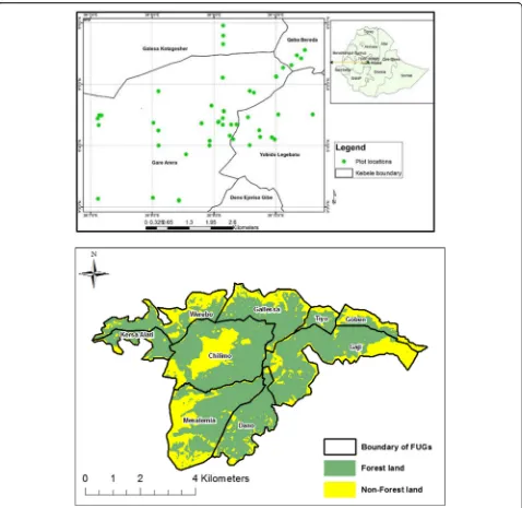
The Chilimo forest contains a total of 4500 ha. For ad-ministrative purposes, the forest has been partitioned into nine compartments (forest patches) as a part of the management scheme of Oromia Forest and Wildlife
En-terprise (Fig.1). This study was conducted in the largest
forest patches of the forest which are Chilimo, Galless, and Gaji. The sampled plots are geographically located
at 038° 08′ 679′′ to 038° 10′ 283′′ E latitude and 09°
04′ 038′′to 09°05′765′′ N longitude, at an altitude of
2470 to 2900 m above sea level (Fig.1) in Dendi District,
Western Shewa Zone, Oromia Administrative Region, and Central Highlands of Ethiopia. Chilimo forest is one of the few remnant of dry afromontane forests located in the Central Highlands of Ethiopia. This forest is charac-terized by a small enclave in the western section of a chain of hills and ridges that stretch over 200 km from north of Addis Ababa westwards up to the Ghedeo high-lands in the west, and local river valleys and gorges cut through the chain. Awash river, one of the longest river in the country, originates from this forest and is the home of over 180 species of birds and 21 species of
mammals (Woldemariam 1998). Chilimo forest is
com-posed of mixed broad-leaved Podocarpus falcatus, Olea
europaea, Scolopia theifolia, Rhus glutinosa, Olinia rochetiana, and Allophylus abyssinicus, and Juniperus procera are the major species in the forest (Bekele2004;
Kelbessa and Soromessa 2004; Kassa et al. 2008). While
Shumi (2009) investigated 42 species composed of 27
tree and 15 shrub species in the forest, Tesfaye (2015)
reported for Chilimo 33 different native woody species (22 tree species and 11 shrub species) in three forest
patches. On their part, Soromessa and Kelbessa (2014)
reported 213 different plant species which belong to 83 families, and 18 plant species are recorded as endemic, from which one was endangered and three were evalu-ated as vulnerable to the Chilimo forest (Kelbessa and
Soromessa2004).
For over a century, Chilimo forest was owned and controlled by the State. Nevertheless, the State control had weakened from 1991 to 1996. This resulted in an in-creasing conversion of the forest into agricultural land and illegal cutting of trees for timber, construction wood, and fuelwood. Thus to minimize deforestation of the remaining forest, the government classified 58 natural forests as National Forest Priority Areas NFPAS in
mean annual temperature of the area ranges between 15 and 20 °C, and the mean annual precipitation ranges
from 1000 to 1264 mm (Shumi 2009). Following
Köppen’s classification, the climate of Chilimo forest
could be classified as warm temperate climate I
(CWB) type (EMA 1988).
Field sampling
Reconnaissance survey
Discussions were held with Oromia Wildlife and Forest Enterprise office in Addis Ababa for awareness creation and issuance of authorizations to work in this forest. Subsequently, after the permit, a reconnaissance survey
was conducted through a field visit and a physical obser-vation across the forest. Three forest patches were selected for further in-depth study based on their acces-sibility, species composition, and representativeness. Then an inventory was conducted in Chilimo, Gallessa, and Gaji forest patches. The survey also covered the ad-jacent land-use types, which include plantation forests, cultivated land, and degraded lands.
Sampling design
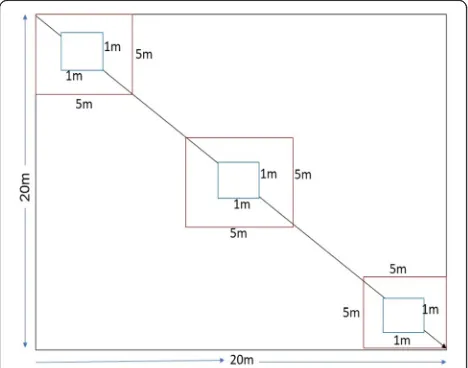
A systematic sampling approach was used to carry out
the inventory. A total of 35 20 m × 20 m (400 m2)
squared sampled plots (20 plots in Chilimo, 11 plots in
Gallessa, and 4 plots in Gaji forest patches) were
estab-lished, based on Neyman’s optimal proportional
alloca-tion formula in the natural forest (Kangas and Maltamo
2006; Köhl et al. 2006) (Fig. 2). In addition, nine sample
plots of 20 m × 20 m were established in the plantation of Cupressus lusitanica, Eucalyptus saligna, and Pinus patula forests (three in each) along an altitudinal gradi-ent. Additionally, six plots under cultivated land and degraded land (three in each) were laid out for soil sam-pling. The total number of plots was 50 in natural and plantation forests and cultivated and degraded lands. The center of the first plot was laid out systematically using Silva compass, 150 m away from the outer edge following north direction to avoid edging effect. To at-tain a 90°corner of the main plots, the Pythagoras the-orem was applied. Then, four sharpened wooden pegs were stalked in the four corners of the main plot. The plots were laid out along 100 m ground distance, starting from the highest to the lowest ridges of the mountains using a measuring tape, GPS, and compass. A total of ten transect lines (four in Chilimo, four in Gallessa, and two in Gaji) were made along the center of the natural forest. The distance between two consecutive transect lines was 300 m and 1 km, respectively, depending on the accessibility of the next transect. A first inventory was conducted in 2012, and remeasurements were con-ducted within the same established sampling plots and for the same numbered trees in 2017. Soil samples were also taken from adjacent land-use types (cultivated land and degraded land) 1 km away from the outer edge of the natural forest. The horizontal distance between sam-pling plots in these land-use types was also 100 m, and transect lines were made from bottom to top parts of the gradient.
Field data collection
Before the actual measurements started, all trees and shrubs found in the border of each plot were marked, and then, all trees in the main plot were numbered.
Indi-vidual species were categorized into trees (≥5 cm
diam-eter at breast height [DBH]), shrubs, saplings (height ≥
1.3 m and DBH 2.5–5 cm), and seedlings (height 0.30–
1.3 m and DBH≤2.5 cm) following Lamprecht’s
classifi-cation (Lamprecht1989). Tree measurements were
con-ducted in the 20 m × 20 m main plot, while shrubs and saplings were measured in 3.5 m × 5 m subplots and seedling measurements were made in 3.1 m × 1 m sub-plots. Tree diameter (cm) was measured using a metallic caliper for small- and medium-sized trees, while diam-eter tape was used for bigger tree measurements. Height was measured to the nearest two digits using Vertex III digital electronics tree height measurement instruments. In cases where trees branched at below the breast height, the diameter was measured separately for each branch and was the square root of diameter squared (pffiffiffiffiffiffiffiffiffiffiffiffiffiffiffiffiffiffiffiffiffiffiffiffiffiffiffiffiffiffiffiffiffiDbhi2þDbhii2). Likewise, the diameter at each stem was measured separately for trees with multiple stems connecting near to the ground. For irregular-ities and/or buttresses on large trunks, measure-ments were taken at the nearest lower points. Height and diameter measurements for shrubs and saplings were done using graduated wooden bars and metallic caliper. Counting and average height measurement for seedlings were made using a wooden ruler.
Data analysis
For the purpose of analysis, environmental factors and forest patches were categorized into three discrete
clas-ses: the altitudinal gradient as class 1 (low elevation) ≤
2599 m, class 2 (middle elevation) 2600–2699 m, and
class 3 (high elevation)≥2700 m and slope class as slope
1 (gentle slope) ≤25%, slope 2 (middle slope) 26–50%,
and slope 3 (steep slope) 51–70%; data for the different
carbon pools both in the natural forest and other land uses were analyzed using RStudio (R-Development Core
team, 2017). To analyze the equality of means, we used
ANOVA for multiple comparisons among elevation
classes at α= 0.05.
Aboveground biomass
Aboveground biomass was calculated using the equation
of Chave et al. (2014) (Eq.1)
AGB¼0:0673ðρHDbh2Þ^0:976 ð1Þ
where AGB is the above ground biomass (in kg), Dbh is
the diameter at breast height (in cm),His the height (in
m), and ρ is the basic wood density (in g cm−3). The
wood density data information were obtained from the
Global Wood Density Database (Zanne et al. 2009),
ICRAF Wood Density Database (www.worldagroforestry.
org), and Wood Technology Research Centre, Addis
Ababa (Desalegn et al.2012). In addition, wood densitity
for Allophyllus abyssinicus, Olea europea subspp cuspi-diata, Olinia rochetiana, Rhus glutinous, and Scolopia theifoliawas used from Tesfaye (2015).
Accumulated aboveground and total carbon density
was calculated following Eqs.2and3:
ACD¼AGB0:47 ð2Þ
(IPCC2006)
BCD¼ACD0:24 ð3Þ
(Gibbs et al.2007; Ponce-Hernandez2004)
where ACD is the aboveground carbon density (t C ha−1)
and BCD is the belowground carbon density (t C ha−1).
The accumulated aboveground and total carbon dens-ities for each tree were calculated separately in each plot, and then, figures for the carbon density of each tree were summed up to give a plot accumulated carbon density and converted to per hectare. The plots were stratified along altitudinal gradient, slope percent, forest patch, and land-use types using R software
(R-Develop-ment Core Team2017).
Herbaceous biomass sampling and analysis
Sampling at the herbaceous layer was made in the inter-ior of three subplots for the inventory of herbs and grasses in 2017. Harvesting of herbs and grasses was made using sickles, and fresh weight of all samples was recorded in the field using string balance. Then, 500 g of fresh sample was taken to the laboratory to determine the water content and dry biomass.
The samples were oven dried at 70 °C for 24 h and weighed again to obtain the dry matter of the sample,
and these data were used for the calculation of Eq.4:
HbCD¼ WsampleðdryÞ
= WsampleðfreshÞ
Wfield=30:4710000=106 ð4Þ
where HbCD is the herbaceous carbon density (t C ha−1),
Wsample (dry) is the sample oven-dried weight, Wsample
(fresh) is the sample fresh weight, and WFieldis the total
fresh weight of the samples collected.
Coarse wood debris sampling
Deadwood was sampled in 11, 6, and 1 plots in Chilimo, Gallessa, and Gaji forest patches, respectively. Coarse wood debris (logs and cut stumps) were inventoried within the 20 m × 20 m plots. All fallen branches and/or twigs of 2 cm diameter and above were collected and measured in the field using string balance. The weight of big logs was estimated in the field manually. For fallen
branches and twigs, subsamples were taken into the la-boratory. All fallen branches/twigs of 2 cm diameter and above were oven dried at 102 °C for 24 h.
Stump biomass
Stumps were sampled inside the 20 m × 20 m plots. Diameter measurements for all the stumps were made in the main plots in their bases and at the top using a me-tallic caliper and diameter tape, while height measure-ments were done using a measuring tape. To calculate the stump carbon, first, the volume was calculated using
Smalian’s formula (Nicholas et al.2012) (Eq.5):
V¼π=8L D12þD22
ð5Þ
whereVis the volume (cm3),Lis the length of the trunk
(cm),D12is the diameter of the narrow end of the trunk
(cm), and D22 is the diameter of the large end of the
trunk (cm). Once the volume was determined, the mass
was calculated as follows (Eq.6):
mi¼ρiVi ð6Þ
wheremiis the mass in kilograms,ρiis the density (g cm−3), andViis the volume.
Forest floor and litter sampling and analysis
Litter, intermediate, and humus samples were taken
within a 0.25 m × 0.25 m (0.0625 m2) metallic frame in
the center of the main plot where available, while depth of the forest floor was measured using a metallic ruler. The collected materials were taken into the laboratory for analysis for water content and dry weight.
The sampled litter, intermediate, and humus layers were oven dried at 70 °C for 24 h in the laboratory and weighed using sensitive balance. Chemical analysis for the humus and intermediate layer was performed using
the loss-on-ignition method (Ben-Dar and Banin 1989).
Then, soil organic matter was converted into organic
carbon following Eq.7and Eq.8:
SOM¼ðw105−w400Þ=w105100 ð7Þ
%C¼%SOM0:58 ð8Þ
where SOC is the soil organic carbon concentration, SOM is the soil organic matter, w105 is the weight of dry soil sample at 105 °C, w400 is the weight of ground soil sample at 400 °C, and 0.58 is the carbon concentra-tion in the soil organic matter which has been found to be the most convenient conversion factor from organic matter to carbon content in forest floor (De Vos et al.
The forest carbon density was calculated using the
con-version of humus carbon stock density (HuCD, in t C ha−1)
in the sampled plot following Eq.9:
HuCD t C ha −1¼HODweight 0:0625
cp
10010000=10^6 ð9Þ
where HuCD is the humus carbon density, HOD is the
humus oven dry weight, and Cp is the carbon
percentage.
Soil organic carbon sampling and analysis
Mineral soil samples were collected in 18 out of 50 sam-pled plots in natural forest, 9 in plantations, 3 in culti-vated lands, and 3 in degraded lands. Sampling was made layer by layer with 1-m-long × 0.60-m-wide dug
pit at the center of the main plot. Five hundred grams
each of four mineral soil layers (0–10, 10–30, 30–50,
and 50–100) was sampled and handled with plastic bags.
Separate samples were taken at four soil depths for bulk density with a 5-cm-high cylinder that was introduced vertically in the corresponding depth. Resamplings were made in both cases by digging new sample pits 10 cm away from the older pit following an appropriate direc-tion. A total of 264 (132 mineral soil + 132 cores) were collected and transported into the laboratory for organic C % and bulk density analyses.
Mineral soil sampled was air dried and passed through a 2-mm sieve to obtain the fine fraction for chemical analysis. The coarse fragments (2 mm) were removed from the sample, and their percentage of stoniness and
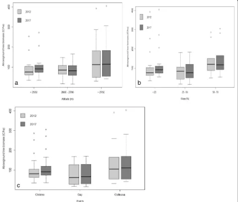
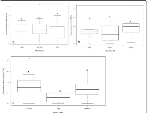
Fig. 3a–cAboveground biomass (t C ha−1) along the altitudinal gradient, slope, and forest patch (capital letter indicated the significant difference
or rockiness was calculated by comparing their mass with the total weight of the oven dried samples at 67 °C
for 24 h (Eq.10):
CFW%¼weight coarse fraction
weight of total soil 100 ð10Þ
where CFW is the percentage of coarse fragments by weight (Page-Dumroese et al. 1995). Then, the total or-ganic carbon (C %) was analyzed following
Walkley-Black’s method described by the Anderson and Ingram
(1996) procedure. Bulk density was estimated following
the procedure of Blake (1965). The oven-dried soil
was weighed and divided by the volume of the metal-lic cylinder.
The SOC stock density in mineral soil was calculated
based on fixed depth method using carbon
concentration, thickness of each layer, soil bulk density, and coarse fragmented matter at each depth, according
to Eq.10(Ruiz-Peinado et al.2013) (Eq.11):
SOC stock¼SOC con:BD:Lð1−CFMÞ 10 ð11Þ
where SOC stock is the soil organic carbon per unit area
(t C ha−1), SOC con. is the carbon concentration in the
soil layer (kg C t−1 soil), BD is the bulk density (t soil
m−3),Lis the depth of the sample layer (m), CFM is the
percent mass coarse fragmented matter > 2 mm, and the multiplying factor 10 is required to express the result in correct units.
Total forest ecosystem carbon estimation
The total carbon stock (carbon density) was calculated by summing up all the seven carbon stocks of each
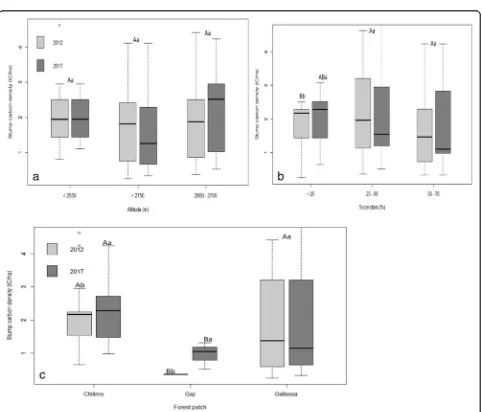
Fig. 4a–cStump carbon density (t C ha−1) along the altitudinal gradient, slope range, and forest patch (capital letter indicated the significant
carbon pools of the forest ecosystem following Pearson
et al. (2005), then converted into tonnes of CO2
equiva-lent by multiplying it by 3.67 as developed by Pearson et
al. (2007). Carbon stock density of the study area was
calculated using (Eq.12):
TECD¼ACDþBCDþDWCDþStCD
þHbCDþLCDþHuCDþSOCD ð12Þ
where TECD is the total ecosystem carbon density (t C
ha−1), ACD is the aboveground carbon density (t C ha−1),
BCD is the belowground carbon density (t C ha−1),
DWCD is the deadwood carbon density (t C ha−1), StCD
is the stump carbon density (t C ha−1), LCD is the litter
carbon density (t C ha−1), HuCD is the humus carbon
density (t C ha−1), HbCD is the herbaceous carbon
dens-ity (t C ha−1), and SOCD is the soil organic carbon
dens-ity (t C ha−1).
Correlation and regression analyses
A multiple regression correlation analysis was performed
using R software (R-Development Core Team 2017).
Then, a multiple regression correlation matrix graph was developed. Highly correlated carbon pools were se-lected and further evaluated. A linear correlation ana-lysis graph and a linear equation model were developed, evaluated, and fitted. The best linear models were se-lected based on the MRES (mean residual for evaluating bias) and the RMSE (root mean square error for evaluat-ing precision).
Results
Aboveground biomass and belowground carbon biomass
The aboveground and belowground biomass varied sig-nificantly among the altitudinal gradient and slope
per-centP≤0.05. However, there was non-significant among
time and forest patch (Table 2; Fig. 3a–c). The
above-ground and belowabove-ground biomass was the highest for
Fig. 5a–cHerbaceous carbon density (t C ha−1) along the altitudinal gradient, slope percent, and forest patch (capital letter indicated the significant
Table 1 The different carbon pools of Chilimo dry afromontane forest natural forest along the altitudinal gradient, slope, and forest patch (mean ± SD) Factors Level ACD (t C ha − 1) BCD (t C ha − 1) StCD (t C ha − 1) Deadwood (tC
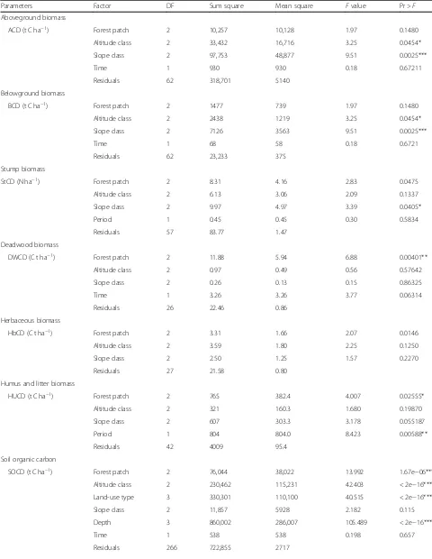
Table 2ANOVA for the five carbon pools of the Chilimo dry afromontane forest along the altitude, slope, and forest patch
Parameters Factor DF Sum square Mean square Fvalue Pr >F
Aboveground biomass
ACD (t C ha−1) Forest patch 2 10,257 10,128 1.97 0.1480
Altitude class 2 33,432 16,716 3.25 0.0454*
Slope class 2 97,753 48,877 9.51 0.0025***
Time 1 930 930 0.18 0.67211
Residuals 62 318,701 5140
Belowground biomass
BCD (t C ha−1) Forest patch 2 1477 739 1.97 0.1480
Altitude class 2 2438 1219 3.25 0.0454*
Slope class 2 7126 3563 9.51 0.0025***
Time 1 68 58 0.18 0.6721
Residuals 62 23,233 375
Stump biomass
StCD (N ha−1
) Forest patch 2 8.31 4.16 2.83 0.0475
Altitude class 2 6.13 3.06 2.09 0.1337
Slope class 2 9.97 4.97 3.39 0.0405*
Period 1 0.45 0.45 0.30 0.5834
Residuals 57 83.77 1.47
Deadwood biomass
DWCD (C t ha−1) Forest patch 2 11.88 5.94 6.88 0.00401**
Altitude class 2 0.97 0.49 0.56 0.57642
Slope class 2 0.26 0.13 0.15 0.86325
Time 1 3.26 3.26 3.77 0.06314
Residuals 26 22.46 0.86
Herbaceous biomass
HbCD (C t ha−1) Forest patch 2 3.31 1.66 2.07 0.0146
Altitude class 2 3.59 1.80 2.25 0.1250
Slope class 2 2.50 1.25 1.57 0.2270
Residuals 27 21.58 0.80
Humus and litter biomass
HUCD (t C ha−1
) Forest patch 2 765 382.4 4.007 0.02555*
Altitude class 2 321 160.3 1.680 0.19870
Slope class 2 607 303.3 3.178 0.055187
Period 1 804 804.0 8.423 0.00588**
Residuals 42 4009 95.4
Soil organic carbon
SOCD (t C ha−1) Forest patch 2 76,044 38,022 13.992 1.67e−06***
Altitude class 2 230,462 115,231 42.403 < 2e−16***
Land-use type 3 330,301 110,100 40.515 < 2e−16***
Slope class 2 11,857 5928 2.182 0.115
Depth 3 860,002 286,007 105.489 < 2e−16***
Time 1 538 538 0.198 0.657
the highest altitudinal gradients and the lowest for the medium altitudinal gradients in all the measurement times. The mean aboveground and belowground bio-mass in 2012 for the natural forest was ranged from 139.66 ± 111.44 and 37.71 ± 30.09 for high altitude to 97.49 ± 31.10 and 26.32 ± 8.40 for middle altitude, and in 2017, it was ranged from 148.30 ± 115.02 and 40.03 ± 31.06 for high altitude to 100.14 ± 39.93 and 27.04 ± 10.78 for middle altitudinal gradient. The mean ACD
and BCD was also highest at 151.35 ± 108.98 t C ha−1for
gentle slope and lowest at 88.01 ± 49.72 t C ha−1for
mid-dle slope. In a similar way, the ACD and BCD were highest for Gallessa forest patch and lowest for Gaji for-est patch in all the measurement times. Overall, the ACD and BCD affirmed temporal variations among
alti-tudinal gradient and slope (Fig.3b, c).
Stump carbon biomass
The stump carbon density of the natural forest varied
significantly along slope range and forest patch at P≤
0.05. However, it was non-significant among the
altitud-inal gradient and time (Table 2). The mean stump
car-bon density 2.38 ± 1.45 was highest for the middle
altitudinal gradient and 1.81 ± 1.03 tCha−1was lowest for
the highest altitudinal gradient. Stump carbon density also decreased along with the increasing and decreasing altitudinal gradients and slope range. The mean stump
carbon density 2.33 ± 1.64 t C ha−1 was highest for the
middle slope and 1.68 ± 1.21 t C ha−1was lowest for the
steep slope range. The mean stump carbon density 2.32
± 1.1 tCha−1for the Chilimo forest patch was always the
highest, while 0.68 ± 0.3 tCha−1for the Gaji forest patch
was the lowest. The stump carbon density was also higher in 2017 than in 2012. Moreover, stump carbon density was influenced by the altitudinal gradient, slope
percent, and forest patch (Fig.4a–c). The stump carbon
density among the middle and highest altitudinal gradi-ent was non-significant. The stump carbon density in the Gaji forest patch with others and gentle slope
with other slopes were also significant (Fig. 4a, c).
Harbaceous carbon biomass
The analysis of variance for herbaceous carbon density revealed significant variations among the forest patch
P≤0.05; however, it was non-significant among the
alti-tudinal gradient and slope percent (Table 2). The mean
1.56 ± 1.08 tCha−1 herbaceous carbon density was the
highest under the lowest altitudinal gradient, while 1.27
± 0.94 t C ha−1was the lowest under the middle
altitud-inal gradient. Moreover, the herbaceous carbon density showed an increasing trend along with increasing slope
percentage (Table 4). The highest herbaceous carbon
density was found under the Chilimo forest patch, whereas the lowest was found under the Gaji forest
patches (Table4). The herbaceous carbon density along
the altitudinal gradient, slope percent, and forest patch
is also presented under Fig. 5a–c. There was also a
sig-nificant variation among the Gaji forest patch with Chi-limo and Gallessa; however, it was non-significant among the altitudinal gradient and slope percent
(Fig.5a–c).
Deadwood carbon pool
The analysis of variance for deadwood carbon density is
presented in Table 1 and non-significant among
altitud-inal gradient and slope percent atP≤0.05 (Table2). The
highest 1.58 ± 0.98 tCha−1deadwood carbon density was
found under the highest altitudinal gradient, while the
lowest 0.37 ± 0.21 t C ha−1 was found under the lowest
altitudinal gradient. Moreover, there was an increasing trend along with an increasing altitudinal gradient. The
highest 1.44 ± 2.21 tCha−1deadwood carbon density was
found under the middle slope range, and the lowest 0.21
± 0.20 t C ha−1 was found under the lowest slope range.
Altitude, slope, and forest patch significantly influenced the deadwood carbon density of Chilimo dry
afromon-tane forest at P≤0.05. In line with, the highest 5.88
tCha−1 deadwood carbon density was found under the
Gaji forest patch; however, the lowest 0.26 ± 0.19
tCha−1 was found under the Chilimo forest patch
(Table 3; Fig. 6c).
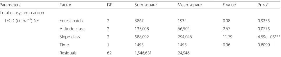
Table 2ANOVA for the five carbon pools of the Chilimo dry afromontane forest along the altitude, slope, and forest patch(Continued)
Parameters Factor DF Sum square Mean square Fvalue Pr >F
Total ecosystem carbon
TECD (t C ha−1) NF Forest patch 2 3867 1934 0.08 0.9255
Altitude class 2 133,008 66,504 2.67 0.0775
Slope class 2 588,092 294,046 11.79 4.59e−05***
Time 1 1455 1455 0.06 0.8099
Residuals 62 1,546,631 24,946
Where:ACDAbove ground carbon density,DFDegree of freedom,HbCDHerbaceous carbon density,StCDStump carbon density,DWCDDead wood carbon density,NFNatural forest,HUCDHumus carbon density,SOCDSoil organic carbon density,tCha-1
Humus and litter carbon pools
The humus carbon density of the forest floor along alti-tudinal gradients was ranged from 17.33 ± 17.35 to 4.84
± 2.58 t C ha−1. The analysis of variance also revealed
that the humus carbon density was significantly
influenced by the forest patch, year of data collected,
and slope percent (P≤0.05) (Table 2). It was highest
for the Gallessa forest patch, but lowest for the
Chilimo forest patch (Table 1; Fig. 7c). The highest
humus and litter carbon stock density was found
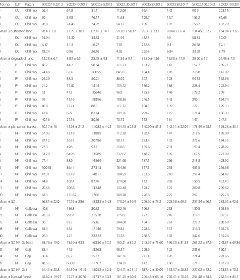
Table 3Soil organic carbon density (SOCD) (t C ha−1) along land use types
Plot no. LUT Patch SOCD.10.2012 SOCD.10.2017 SOCD.30.2012 SOCD.30.2017 SOCD.50.2012 SOCD.50.2017 SOCD.100.2012 SOCD.100.2017
1 CU Chilimo 26.4 64.8 51.1 112.03 66.4 142 90.9 223.15
2 CU Chilimo 30 5.98 76.17 11.68 103.7 15.7 156.2 81.68
3 CU Chilimo 28.8 24.48 74.97 54.12 109 107 156.2 187.29
Mean ± cultivated land 28.4 ± 1.8 31.75 ± 30.1 67.41 ± 14.1 59.28 ± 50.37 93.03 ± 23.2 88.44 ± 65.4 134.45 ± 37.7 164.04 ± 73.6
1 DL Chilimo 14.94 13.39 34.83 21.95 48.33 39 58.83 57.05
2 DL Chilimo 6.37 3.13 16.27 7.81 21.88 9.3 26.68 12.1
3 DL Chilimo 18.24 0.96 26.16 4.92 29.68 6.84 33.28 8.79
Mean ± degraded land 13.28 ± 6.1 5.83 ± 6.6 25.75 ± 9.3 11.56 ± 9.1 33.30 ± 13.6 18.38 ± 17.9 39.60 ± 17 25.98 ± 7.0
1 PF Chilimo 46.2 44.2 98.64 111.23 133.2 142 157.2 209.21
2 PF Chilimo 74.48 63.6 160.59 84.58 184.4 118 216.8 141.82
3 PF Chilimo 24.29 38.3 50.21 88.92 67.1 123 94.33 162.96
4 PF Chilimo 71.2 71.82 141.4 155.12 186.2 188 228.4 222.94
5 PF Chilimo 53 47.3 106.46 96.8 135.3 146 178.2 209
6 PF Chilimo 59 43.46 188.96 108.36 246.1 143 296.1 164.74
7 PF Chilimo 40.8 71.24 88.3 111.72 104.5 139 122 195.33
8 PF Chilimo 42.4 6.72 82.14 109.76 99.42 119 121.4 186.03
9 PF Chilimo 40.16 27.16 80.66 70.72 112 161 147 247.5
Mean ± plantation forest 50.17 ± 16 45.98 ± 21.2 110.82 ± 44.2 104.13 ± 23.8 140.90 ± 55.3 142.11 ± 22.07 173.49 ± 63.1 193.28 ± 33.1
1 NF Chilimo 67.03 72.19 138.89 112.28 192.4 147 217.5 199.09
2 NF Chilimo 87.12 26.75 207.86 90.11 283.4 132 372.6 194.35
3 NF Chilimo 27.3 49.8 92.1 150.6 139.6 233 195.4 278.92
4 NF Chilimo 83.79 64.98 135.89 137.67 148.7 195 167.9 222.09
5 NF Chilimo 77.4 88.9 145.69 221.98 187.5 296 213.8 428.92
8 NF Chilimo 100.35 86.44 273.15 184.36 357.5 235 451.5 256.68
11 NF Chilimo 47.31 83.79 148.11 184.59 233.6 210 297.4 264.42
14 NF Chilimo 44.8 102.4 87.49 279.04 112 358 150.5 452.45
17 NF Chilimo 70.66 70.66 132.48 132.48 174.7 175 209.8 209.82
20 NF Chilimo 62.3 131.67 176.6 209.28 226.8 275 297 329.78
Mean ± SD 66.81 ± 22.0 77.76 ± 28.6 153.83 ± 54.8 170.24 ± 56.9 205.62 ± 73.2 225.58 ± 69.9 257.34 ± 96.1 283.65 ± 92.6
21 NF Gallessa 40.8 136.8 80.32 202.16 106.3 258 130.8 305.86
23 NF Gallessa 78.38 99.81 215.18 225.81 272.3 245 313.1 301.51
25 NF Gallessa 50 82.5 153.6 244.68 184 263 223.2 288.69
28 NF Gallessa 83.3 46.4 171.46 79.84 228.6 112 316.3 192.76
30 NF Gallessa 76.3 27.5 222.22 73.58 288.6 103 342.6 155.24
Mean ± SD NF Gallessa 65.76 ± 19.0 78.60 ± 43.3 168.56 ± 57.2 165.21 ± 82.2 215.97 ± 73.60 196.30 ± 81.33 265.22 ± 87.64 248.81 ± 69.86
32 NF Gaji 85.4 47.6 182.68 98.37 208.6 122 235.6 160.1
34 NF Gaji 50.4 85.2 151.2 141.36 211.4 178 274.4 293.66
35 NF Gaji 48.55 60.09 117.67 134.39 142.3 160 171.1 187.78
Mean ± SD NF Gaji 61.45 ± 20.8 64.30 ± 19.15 150.52 ± 32.5 124.71 ± 23.17 187.42 ± 39.09 153.37 ± 28.85 227.02 ± 52.2 213.85 ± 70.5
Mean ± Natural forest 65.62 ± 19.97 75.75 ± 30.76 157.37 ± 50.3 161.25 ± 60.4 205.46 ± 66.16 205.41 ± 70.56 254.48 ± 84.8 262.34 ± 83.7
under the middle slope range and showed similar
trends with gentle and steep slope ranges (Table 1;
Fig. 7b). There was significant difference among
mid-dle slope with gentle slope and Gallessa forest patch
with Chilimo forest patch; however, it was
non-significant among altitudinal gradients and within
the same altitudinal gradient (Fig. 7 a–c).
Soil organic carbon pool
The SOC stock is highly influenced by the altitudinal gradient, slope range, and forest patch. The analysis of
variance of soil organic carbon is presented in Table 2.
The SOCD was significantly different among the
altitud-inal gradient, slope, and land-use types at P≤0.05. The
SOCD up to 1 m depth was highest at 295.96 ± 80.45 t C
ha−1under the middle altitudinal gradient, but lowest at
206.40 ± 65.59 t C ha−1under the lower altitudinal
gradi-ent (Additional file1: Table S1; Fig.9).
The SOCD up to 1 m depth of the forest patch ranged from 283.65 ± 92.62 for the Chilimo forest patch to
213.85 ± 70.49 t C ha−1for the Gaji forest patch (Table1;
Fig.10b). SOCD among the Chilimo and Gallessa forest
patch was significant; however, SOCD among the same forest patches with time bound and Gaji forest patch
with others was non-significant (Fig. 9b). The SOCD
271.14 ± 60.22 t C ha−1in 2012 was the highest under the
steep slopes; however, 245.48 ± 83.25 t C ha−1 was the
lowest under the middle slope. In 2017, the SOCD 311.91 ± 104.97 was the highest under the gentle slope;
however, 245.48 ± 83.25 t C ha−1 was the lowest under
the middle slope. Moreover, the SOCD was also sig-nificant among steep slopes and middle slopes; how-ever, it was non-significant among the same slope
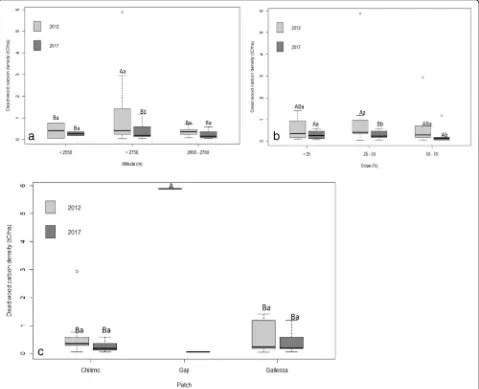
Fig. 6a–cDeadwood carbon density (t C ha−1) along the altitudinal gradient, slope percent, and forest patch (capital letter indicated the significant
range with time bound and gentle slope with others,
respectively (Fig. 8c).
The soil organic carbon stock density was highly
in-fluenced by land-use types and soil depth (Table 2).
The SOCD up to 1 m depth was ranged from 254.48
± 84.8 t C ha−1for natural forests to 39.60 ± 17 t C ha−1
for degraded lands. Similarly, the SOCD in 2017 was ranged from 262.34 ± 83.7 for natural forests to 25
98 ± 7 t C ha−1 for degraded lands. The mean SOCD
up to 1 m nominal depth of the natural forest was
also 264.44 ± 84.81 and 277.77 ± 83.73 t C ha−1 in 2012
and 2017, respectively (Annex 1). the SOCD in the natural forest was always higher than other land-use types in all soil depth. On the contrary, the SOCD in
the degraded and cultivated land was the lowest in all soil depth in all the measurement times (Annex 1). Moreover, the SOCD of the natural forest was signifi-cantly different among other land-use types and
al-ways higher in all soil depth (Table 1 and Fig. 8d).
On the contrary, SOCD for the degraded land was the lowest in all soil depth in all the measurement times (Annex 1). The SOCD between the cultivated land and plantation forest was non-significant, al-though the value of plantation forest was higher than cultivated land. In plantations, the carbon stock dens-ity at the same depth was one third less than natural forests but 35% and 77% higher than cropland and degraded lands, respectively (Annex 1).
Fig. 8a–cSoil organic carbon density (t C ha−1) along the altitudinal gradient, slope percent, and forest patch (capital letter indicated the significant difference among the altitudinal gradient and slope percent)
Table 4The linear regression equation of the different carbon pools of Chilimo dry afromontane forest
SN Equation SE tvalue Pr > /t/ Adj.R2
1 HUCD2012 =−0.6563 + 41.6202DWCD2012 0.60 0.21
−1.09 34.36
0.286 < 2e−16***
0.98
2 HUCD2017 =−1.0623 + 20.5616HbCD2017 0.37
0.74 −
2.86 27.85
0.00887** < 2e−16***
0.97
3 HUCD2017 =−0.6336 + 20.2528DWCD2012 0.25
0.49 −
2.59 41.00
0.0166* < 2e−16***
0.97
4 HbCD2017 = 0.0461198 + 0.0230173HUCD2012 0.01 0.001
3.29 33.20
0.00324** < 2e−16***
0.98
5 HbCD2017 = 0.02648 + 0.97002 DWCD2012 0.01 0.03
2.15 39.05
0.0424* < 2e−16***
0.99
6 StCD2012 = 0.25923 + 0.72541StCD2017 0.18 0.08
1.461 9.152
0.151 1.4e−11***
0.66
Is there any correlation among carbon pools in the natural forest?
The multiple regression correlation matrix and lin-ear relationship of various carbon pools in the
Chilimo forest ecosystem are presented in Table 3
and affirmed the linear relationship among carbon pools. Based on the goodness-of-fit statistics and biological behavior of the model, there was a strong linear relationship between the weighted above-ground, humus, herbaceous, and deadwood carbon density which was highly correlated with the
ad-justed R2 (> 0.97) (Tables 3 and 4). There was also a
moderate linear relationship between the soil organic
carbon stock density and the adjusted R2 (> 0.60).
However, there was a weak linear relationship between
stump carbon density and topsoil carbon density, above-ground carbon density and herbaceous carbon density, and aboveground carbon density and stump carbon
dens-ity (Fig.9a–d).
Do environmental factors and forest patch affect total ecosystem carbon?
The results affirmed that the total ecosystem carbon was significantly influenced by environmental factors and
forest patch atP≤0.05. The highest total ecosystem
car-bon stock density was found under the highest altitud-inal gradient, highest slopes, and Gallessa forest patch
(Fig. 10 a–c). The total ecosystem carbon density was
significant among the middle and highest altitudinal gra-dient, the middle slope with steep and gentle slopes, and
the Gaji forest patch with Chilimo and Gallessa forest
patches (Fig.10a, b). The mean ecosystem carbon stock
density of the sampled plots in natural forests was also ranged from 196.22 to 672.72 and 221.89 to 819.44 t C
ha−1 in 2012 and 2017, respectively (Additional file 1).
The total natural forest and plantation forest were esti-mated to be 5000 and 450 ha, respectively. The sum of the total ecosystem carbon stock density for the natural and
planted forest was 1,564,847 (5,742,996.2 t CO2 eq. in
2012 and 1,660,318 t C or 6,093,365 t CO2 eq. in 2017).
The combined carbon sequestration potential of the Chilimo natural forest and planted forest was also
esti-mated to be 65,828.98 t CO2eq. year−1. The carbon
se-questration potential of the Chilimo natural and planted
forest was estimated to be 65,828.98 CO2eq. year−1.
Discussion
The present study has investigated the temporal vari-ation in carbon pools of the Chilimo dry afromontane
forest along the altitudinal gradient, slope, and forest patch. This study is also the first type in the study area conducted into two consecutive periods. There is a lower aboveground biomass in the middle altitudinal gradient, this is might be due to the intense anthropo-genic effect, which resulted in few but big trees with higher above and belowground biomass. In addition, there is a higher stump carbon density in the middle and lower altitudinal gradient, this is might be due to the presence of higher number of stumps. In line with,
simi-lar reports were also reported by Shumi (2009), Hassen
(20150, Tesfaye (2015), and Tesfaye et al. (2016).
The aboveground biomass carbon density reported
(200 t C ha−1
) in the Chilimo forest is also higher than the Gara Mukitar dry afromontane forest in Eastern
Ethiopia (156.60 t C ha−1) (Wodajo 2018). However, it
was less than by 142.47 and 174.02 t C ha−1of the Arba
Minch riverine forest, Egdu forest, and Gera moist
afro-montane forest (Hassen 2015; Meles et al.2014; Feyissa
et al. 2013), Chato forest (301.86 t C ha−1) (Iticha 2017)
and Ades forest too (259.17 t C ha−1) (Kassahun et al.
2015). The highest ACD (200 t C ha−1) under the higher
altitudinal gradient and slope range is might be due to lower disturbance. Similar findings are also reported for
other Ethiopian forests too (Girma et al. 2004; Hassen
2015; Iticha2017).
The mean accumulated biomass capacity of the Chi-limo forest as mentioned above is also in line with the reports of Eticha et al. (2017). But, it was lower than the
Zequala Monastery (475.51 t C ha−1) and Semien
Moun-tain National Park forest (994.16 t C ha−1) in the Central
and Northern Ethiopia, respectively (Abel Girma et al.
2014; Yelemfrhat et al. 2014). The highest deadwood
carbon density at steep slopes and highest altitudinal gradients is might be due to the low disturbance. More-over, the higher deadwood carbon density in the Gaji forest patch is also due to the presence of big fallen trees in the sampled site than others.
The herbaceous carbon density of the Chilimo forest is in line with other tropical seasonal rain forests (1.4),
tropical secondary forests (1.9) (Lasco et al. 2006), and
subtropical forest too (2.6–3.8 t C ha−1) (Brown et al.
1989). The higher herbaceous carbon density under the
lower and higher altitudinal gradients is also might be due to the low canopy cover. The higher herbaceous car-bon density in steep slopes is also due to the low
dis-turbance and better nutrient release. Swai et al. (2014)
reported low tree density makes a suitable condition for undergrowth, vegetation, and higher precipitation. The reduction in litter and humus carbon is due to an in-creasing disturbance and excessive removal of litterfall.
The soil carbon stock density was conducted across the altitudinal gradient, land-use type, slope, and forest patch for the last 5 years except a study done by Tesfaye
et al. (2016). In this study, the soil carbon stock was
sig-nificant along the altitudinal gradient as suggested by
other studies in African forests too (Zewdu et al. 2004;
Twongyirwe et al. 2013), because altitudinal gradient is
one of the environmental factors that affect the soil car-bon stock density and it can be considered as a useful tool to predict the forest carbon stock (Mayaux et al.
2007). Results of the present study also revealed that
higher soil organic carbon stock density was found under the middle altitudinal gradients. This was might be due to low soil erosion and higher number of inputs. However, the carbon stock in the forest floor showed a reduction in the last 5 years. This is might be due to fre-quent removal of litterfall and twigs by fuelwood collec-tors. At the same time, lower canopy cover might result in high sunlight to reach the forest floor that accelerates
the litter decomposition. Similary, Hassen (2015) found
higher carbon pools in Gera moist afromontane forest due to higher disturbance.
The higher carbon stock density in the middle altitud-inal gradient is might be due to higher disturbance; this
is also in line with Kassahun et al. (2015) who reported
for a higher SOC density under a middle altitudinal gra-dient of Ades dry afromontane forest. The lower carbon stock density in the higher and middle elevation is might be due to the over sealing of soil by livestock movement and higher soil erosion. In addition, there is a continu-ous removal of fallen litter, deadwood, and twigs by fuelwood collectors. Tree cutting for firewood, char-coal making, illegal logging for timber and construc-tion wood, forest clearing for agricultural land, and free livestock grazing are also frequently occurring in these areas.
Land use is a major factor in carbon stock, among the four land-use types studied in the Chilimo dry afromon-tane forest and adjacent land uses. The higher carbon stock in the natural and plantation forest in all the sam-pled period is might be due to higher litterfall, decom-position rate, and species comdecom-position. The low erosion rate in the natural and plantation forest was might be due to the interception of the raindrops by plants. The carbon stock density was slightly reduced in the forest floor in the last 5 years due to the lack of appropriate land management practices to improve land productivity and more tree cutting in the natural forest than previous years. The low carbon in the degraded and cultivated land is might be due to the low nutrient cycling, con-tinuous tillage, and crop residue removal for livestock feed in the cultivated land. In addition, in the degraded land, there is an over sealing and surface crusting effect, which reduced the microbial activity and leads to a high runoff and soil erosion. In general, there is a slight in-crease in the carbon stock in the degraded land in the last 5 years; this is might be due to some exclosure activ-ities done in these areas. Similar results were also reported by several authors; Girmay et al. (2008) reported the
car-bon stock in the topsoil (0–10 cm) is decreased after the
conversion of native forest into croplands (−63%) and
plantations (−83%). Solomon et al. (2002) indicated that
the conversion of humid tropical forests for maize
cultiva-tion in Southern Ethiopia resulted in a 55–60% reduction
in SOC stock. Ashagrie et al. (2005) also reported losses of
13 Mg Cha−1 over a period of 21 years in southern
Ethiopia when natural forest was converted into a
euca-lyptus plantation. In Brazil, Zinn et al. (2002) reported a
23–48% loss in SOC after a native wooded savannah was
converted into a eucalyptus plantation. Rhoades et al.
(2000) reported a 70% reduction in SOC in Ecuador in the
upper 30 cm of the topsoil when the original forest was
converted into a sugarcane plantation (Saccharum spp.).
Berhangaray et al. (2013) investigated the impact of
plantations stored 34% less carbon than native forest, but the land-use change sequence was different. Plantations were originally planted outside the forest on bare or de-graded land. In this situation, tree plantations stored 80% more carbon than degraded lands and 56.4% more carbon than croplands. The C stock density under native natural forest and plantation forest in the Chilimo dry afromon-tane forest was higher than those reported in other
re-gions (Beets et al.2002; Harms et al.2005; Twongyirwe et
al.2013) and suggests two management strategies for
im-proving soil conditions. The first is to maintain and pre-serve the Chilimo natural forest as other African tropical
forests do (Lewis et al.2009), and the second is to recover
abandoned croplands and degraded lands by establishing tree plantations.
There is a strong linear relationship between the humus and herbaceous carbon density due to the pres-ence of higher humus content which is good for the growth of herbaceous plants and higher decomposition rate and open canopy cover. On the contrary, the pres-ence of higher humus content results due to low soil erosion. The strong linear relationship between the humus and deadwood carbon density is might be due to a higher litterfall, better decomposition, and better twigs. The weak linear relationship between the stump and herbaceous carbon density is due to a higher number of stumps, low aboveground carbon density, and lower herbaceous plants.
The total area of Chilimo forest was 22,000 ha in 1982 and reduced to 4500 ha in 2016; as a result, the total car-bon emission for Chilimo forest in the last 34 years was 5,218,850 t C. In general, the mean carbon stock density of Chilimo forest has increased from 289.86 to 298.22 t C
ha−1. In 2012, the total ecosystem carbon density was
56.12% in soil organic carbon, 31.21% aboveground bio-mass, 8.43% belowground biobio-mass, 3.65% humus carbon, 0.47% stump carbon, and 0.12% deadwood carbon. In the same line in 2017, the highest share for ecosystem carbon density was soil organic carbon (59.64%), aboveground carbon (29.78%), belowground carbon (8.04%), humus car-bon (1.69%), stump carcar-bon (0.48%), herbaceous carcar-bon (0.33%), and deadwood carbon (0.04%), respectively.
Conclusions
The aboveground and belowground biomass of the Chilimo natural forest was the highest for the highest altitudinal gradients and the lowest for the medium alti-tudinal gradients in all the measurement times. The stump carbon density was increased in 2017 than in 2012 due to the increasing number of illegal stumps. Deadwood and humus carbon density was reduced by 50% in the last 5 years due to a surplus increasing level of disturbance. The SOCD up to 1 m depth was the
highest at 295.96 ± 80.45 tCha−1 under the middle
altitudinal gradient; however, it was the lowest at 206.40
± 65.59 t C ha−1under the lower altitudinal gradient. The
Chilimo natural forest stored more carbon than adjacent land-use categories, but degraded land stored the lowest soil organic carbon stock. The carbon stock density was weakly correlated among the stump carbon density and aboveground carbon density. The sum of total ecosystem carbon stock density and carbon sequestration potential for the natural and planted forest was 1,660,318 tC or
6,093,365 t CO2eq. and 65,828.98 CO2eq. year−1,
respect-ively. For maintaining a higher carbon stock density in the study area, other land use types such as degraded land and cultivated. Forest management options should be applied to
improve productivity. We recommend a forest
carbon-related awareness creation for local people, and promotion of the local knowledge can be regarded as a pos-sible option for sustainable forest management.
Additional file
Additional file 1:Table S1.Ecosystem carbon accumulation potential of Chilimo dry afromontane forest 2012 and 2017. (DOCX 47 kb)
Abbreviations
°C:Degree Celcius; ACD: Accumulated aboveground carbon density; AGB: Aboveground biomass; ANOVA: Analysis of variance; BCD: Belowground carbon density; C: Carbon; CFW: Coarse fragmented matter; cm: Centimeter; CO2eq: Carbon equivalent; CO2: Carbon dioxide; CU: Cultivated land; Dbh: Diameter at breast height; DL: Degraded land; DWCD: Deadwood carbon density,; g: Gram; Gt: Giga tone; H: Height; HbCD: Herbaceous carbon density; HUCD: Humus carbon density; IPCC: International Panel for Climate Change; Km: Kilometer; LCD: Litter carbon density; LUT: Land-use type; M: Meter; Mg: Megagram; mm: Millimeter; NF: Natural forest; PF: Plantation forest; SD: Standard deviation; SOCD: Soil organic carbon density; StCD: Stump carbon density; t C ha−1: Tonne carbon per hectare; Tg: Teragram; V: Volume; ρ: Basic wood density
Acknowledgements
The authors thanks Genene Tesfaye, Central Ethiopia Environment and Forest Research Centre, for assisting us in field data collection and preparation of plant and soil samples, Mossissa Kebede from Oromiya Forest and Wildlife Enterprise, Ginch Branch and Mekonnen Gemechu from Chilimo village, for their assistance in field work and soil pit digging.
Funding
The Ecosystem Management Research Directorate, Ethiopian Environment and Forest Research Institute (EEFRI) for funding the research grant and the Swiss Government Scholarship programme was given full scholarship for funding to Mehari A.Tesfaye’s fellowship.
Availability of data and materials
The data sets used and analyzed during the current study are available from the corresponding author on reasonable request.
Authors’contributions
Ethics approval and consent to participate
This research was performed in accordance with the laws, guidelines and ethical standards of Ethiopia and Switzerland, where the research was performed.
Competing interests
The authors declare that they have no competing interests.
Publisher’s Note
Springer Nature remains neutral with regard to jurisdictional claims in published maps and institutional affiliations.
Author details
1Ethiopian Environment and Forest Research Institute (EEFRI), Box 24536 code 1000, Gurd Shola, Addis Ababa, Ethiopia.2School of Agricultural, Forest and Food Sciences HAFL, Bern University of Applied Sciences, CH-3052 Zollikofen, Switzerland.
Received: 17 January 2019 Accepted: 21 March 2019
References
Adugna F, Teshome S, Mekuria A. Forest carbon stocks and variations along altitudinal gradients in Egdu forest: implications of managing forests for climate change mitigation. Sc Technol Art Res J. 2013;2(4):40–6.
Anderson JM, Ingram JS. Tropical soils biology and fertility. A hand book of methods. 2nd ed. Wallingford: CAB, International; 1996.
Ashagrie Y, Zech W, Guggenberg G. Transformation ofPodocarpus falcatus
dominated natural forest into a monocultureEucalyptus globulusplantation at Munessa, Ethiopia. Soil organic C, N and S dynamics in primary particle and aggregate-size fractions. Agriculture, ecosystem & environment, vol. 106; 2005. p. 89–98.
Baccini A, Laporte N, Goetz SJ, Sun M, Dong H. A first map of Africa’s above ground biomass derived from satellite imagery. Environ Res Lett. 2008;3: 045011.https://doi.org/10.1088/1748-9326/3/4/045011.
Baker DF. Reassessing carbon sinks. Science. 2007;316:1708–9.
Beets PN, Oliver GR, Clinton PW. Soil carbon protection in podocarp/hardwood forest and effects of conversion to pasture and exotic pine forest. Environ Pollut. 2002;116:S63–73 PMID: 11833919 (PubMed- Indexed for MEDLINE). Bekele M. Forest property rights, the role of the state and institutional exigency:
the Ethiopian experience. Doctoral Thesis. Uppsala: Swedish University of Agricultural Sciences; 2003.
Bekele M. Forest property rights, the role of the state and institutional exigency: the Ethiopian experience. Doctoral Thesis. Uppsala: Swedish University of Agricultural Sciences; 2004.
Ben-Dar E, Banin A. Determination of organic matter in arid-zone soils using a simple loss-on-ignition method. Commun Soil Sci Plant Anal. 1989;20(15–16). https://doi.org/10.1080/100103622890936175.
Berhangaray G, Alvare R, de Paepe J, Caride C, Cantet R. Land use effects on soil carbon in argentine pampas. Geoderma. 2013;192:97–110 https://doi.org/10. 1016/j.geoderma.2012.07.016.
Bhat J, Iqbal K, Kumar M, Negi A, Todaria N. Carbon stock of trees along an elevational gradient in temperate forests of Kedarnath Wildlife Sanctuary. For Sci Pract. 2013;15(2):137–43.
Blake GR. Bulk density. In: Black CA, editor. Methods of soil analysis. Wisconsin: American Society of Agronomy; 1965. p. 374–90.
Bongers F, Tenngkeit T. Degraded forests in Eastern Africa: introduction. In: Bongers F, Tenningkeit T, editors. Degraded forests in Eastern Africa: management and restoration. London: Earthscan Ltd; 2010. p. 1–18. Brown S. Estimating biomass and biomass changes of tropical forests: a primer:
FAO forestry paper 134. United Nations, Rome: FAO; 1997.
Brown SAJ, Gillespie JR, Lugo AE. Biomass estimation methods for tropical forests with application to Forest inventory data.For Sci. 1989;35(4):881–902. Chave J, Réjou-Méchain M, Búrquez A, Chidumayo E, Colgan MS, WBC D,
Vieilleden G. Improved allometric models to estimate the aboveground biomass of tropical trees. Glob Chang Biol. 2014;20:3177–90.https://doi. org/10.1111/gcb.12629.
Chave J, Rieâra B, Dubois M. Estimation of biomass in a neotropical forest of French Guiana: spatial and temporal variability. J Trop Ecol. 2001;17:79–96. Chidumayo E, Okali D, Kowero G, Lrwanou M. Climate change in African forest
and wildlife resources. Nairobi: African Forest Forum; 2011.
De Vos B, Vandecasteele D, Deckers J, Muys B. Capability of loss on ignition as a predictor of total organic carbon in non - calcareous forest soils. Commun Soil Sci Plan Anal. 2005;36:2899–921.
Desalegn G, Abega M, Teketay D, Gezahgne A. Commercial timer species in Ethiopia: characteristics and uses-a handbook for forest industries, construction and energy sectors, foresters and other stakeholders. Addis Ababa: Addis Ababa University Press; 2012.
Diawei L, Zongmin W, Bia Z, Kaishan S, Xiaoyan L, Jiaoyan L, Jiaping L, Fang L, Hongatao D. Spatial distribution of soil organic carbon and analysis of related factors in croplands of the black soil regions, Northeast China, agriculture, ecosystems and environment, vol. 113; 2006. p. 73–81. EMA. National atlas of Ethiopia. Addis Ababa: Ethiopian Mapping Authority; 1988. p. 76. FAO (Food and Agricultural Organization of the United Nations). Global forest
resource assessment. FAO forestry paper 147. Rome: Food and Agriculture Organization of the United Nations; 2005.
Gebre TM. Biomass and soil carbon stocks along elevation gradeints of woodland ecosystems. The case of Liben district, South Ethiopia: WGCF, Shashemene, Ethiopia; 2015. MSc Thesis
Gibbs HK, Brown S, Niles JO, Foley JA. Monitoring and estimating tropical forest carbon stocks: making REDD a reality. Environ Res Lett. 2007;2:045023. Girma A, Soromessa T, Bekele T. Forest carbon stocks in woody plants of mount
Zequalla Monastery and its variation along altitudinal gradient : implication of managing forests for climate change mitigation. Sci Technol Arts Res J. 2004;3(2):133–41.
Girma A, Soromessa T, Bekele T. Forest carbon stocks in woody plants of mount Zequalla Monastery and its variation along altitudinal gradient: implication of managing forests for climate change mitigation. Sci Technol Arts Res J. 2014;3(2): 132–40.
Hamere Y, Teshome S, Mekuria A. Carbon stock analysis along slope and slope aspect gradient in Gedo Forest : implications for climate change mitigation. J Earth Sci Clim Chang. 2015;6:9.
Harms BP, Dalal RC, Cramp AP. Changes in soil carbon and soil nitrogen after tree clearing in the semi-arid range lands of Queensland. Aust J Bot. 2005;53: 639–50.https://doi.org/10.1071/BT04154.
Hassen N. Carbon stock along altitudinal gradient in Gera Moist Evergreen Afromontane forest. MSc Thesis, AAU, Addis Ababa, Ethiopia: South Western Ethiopia; 2015.
Houghton RA. The annual net flux of carbon to the atmosphere from changes in land use 1850˗1990. Tellus B. 1998;51:298–313.
IPCC. Good practice guidance for land-use change and forestry. In: Penman J, Gytarsky M, Hiraishi T, Krup T, Kruger D, Pipatti R, Buendia L, Miwa K, NigaraT TK, Wagner F, editors. IPCC, National Greenhouse Gas Inventories Program. Japan: Published by the Institute of Global Environmental Strategies (IGES); 2003. IPCC. In: Egsleston HS, Buendia L, Miwa K, Ngaran T, Tanabe K, editors. Guidelines
for national greenhouse gas inventories (vol 4, AFOLU). National Greenhouse Gas Inventories Program. Japan: Published; IGES; 2006.
IPCC. Climate change 2007: mitigation of climate change. In: Metz B, Davidson OR, Bosch PR, Dave R, Meyer LA, editors. Contribution of working group III to the 4thassessment report of the intergovernmental panel on climate change. Cambridge: Cambridge University Press; 2007. p. 851.
IPCC. In: Stocker TF, Qin D, Plattner G-K, Tignor M, Allen SK, Boschung J, Nauels A, Xia Y, Bex V, Midgley PM, editors. Climate change 2013: the physical science basis. contribution of working group I to the 5th assessment report of the intergovernmental panel on climate change. United Kingdom and New York: Cambridge University Press, Cambridge; 2013. p. 1535.https://doi.org/10. 1017/CBO9781107415324.
Iticha B. Ecosystem carbon storage and partitioning in Chato afromontane forest. Its climate change mitigation and economic potential. Int J Environ Agric Biotechnol. 2017;2(4):2450–1878.
Kangas A, Maltamo M. Forest inventory methodology and applications : managing forest ecosystems 10. Dordrecht: Springer; 2006.
Kassa AG (2015) Forest carbon stock and variations along environmental gradients in Yeka forest and its implication for climate change mitigation. MSC Thesis, AAU, Graduate progarmme.
Kassa H, Campbell B, Sandewall M, Kebede K, Tesfaye Y, Dessie G, Seifu A, Tadesse M, Garedewe E, Sandwall K. Building future scenarios and covering persisting challenges of participatory forest management in Chilimo forest, Central Ethiopia. J Environ Manag. 2008.https://doi.org/10.1016/j.jenuman. 2008.03.2009.