R E S E A R C H A R T I C L E
Open Access
Filtering data from the collaborative initial
glaucoma treatment study for improved
identification of glaucoma progression
Greggory J Schell
1*, Mariel S Lavieri
1, Joshua D Stein
2and David C Musch
2Abstract
Background: Open-angle glaucoma (OAG) is a prevalent, degenerate ocular disease which can lead to blindness without proper clinical management. The tests used to assess disease progression are susceptible to process and measurement noise. The aim of this study was to develop a methodology which accounts for the inherent noise in the data and improve significant disease progression identification.
Methods: Longitudinal observations from the Collaborative Initial Glaucoma Treatment Study (CIGTS) were used to parameterize and validate a Kalman filter model and logistic regression function. The Kalman filter estimates the true value of biomarkers associated with OAG and forecasts future values of these variables. We develop two logistic regression models via generalized estimating equations (GEE) for calculating the probability of experiencing significant OAG progression: one model based on the raw measurements from CIGTS and another model based on the Kalman filter estimates of the CIGTS data. Receiver operating characteristic (ROC) curves and associated area under the ROC curve (AUC) estimates are calculated using cross-fold validation.
Results: The logistic regression model developed using Kalman filter estimates as data input achieves higher sensitivity and specificity than the model developed using raw measurements. The mean AUC for the Kalman filter-based model is 0.961 while the mean AUC for the raw measurements model is 0.889. Hence, using the probability function generated via Kalman filter estimates and GEE for logistic regression, we are able to more accurately classify patients and instances as experiencing significant OAG progression.
Conclusion: A Kalman filter approach for estimating the true value of OAG biomarkers resulted in data input which improved the accuracy of a logistic regression classification model compared to a model using raw measurements as input. This methodology accounts for process and measurement noise to enable improved discrimination between progression and nonprogression in chronic diseases.
Background
Open angle glaucoma (OAG) is a chronic degenera-tive ocular disease characterized by damage to the optic nerve, which when poorly managed can lead to blind-ness. Glaucoma is the second leading cause of blindness with an estimated 2.2 million adult Americans diagnosed with glaucoma [1,2]. Patients with OAG are monitored regularly via visual field (VF) tests and intraocular pres-sure (IOP) readings [3-8]. Clinicians use the results of
*Correspondence: [email protected]
1Department of Industrial and Operations Engineering, University of Michigan, Ann Arbor, Michigan, USA
Full list of author information is available at the end of the article
these monitoring techniques to determine whether signif-icant disease progression has occurred, i.e. a change in the patient’s disease characteristics which calls for changes in treatment decisions. However, these clinical observations are subject to process and measurement noise. Errors in machine calibration, patient anxiety, human error in administering tests, and variations in measurement tech-nique can all contribute to measurement noise when assessing chronic diseases [9]. Biological variability, like intraday fluctuation of intraocular pressure, is a contribut-ing factor to process noise which can affect the ability to identify significant disease progression [10]. Distin-guishing between signal and noise becomes paramount
when these noisy measurements are used in decision making. While most clinicians (glaucoma specialists in particular) are aware of the variability in VF and IOP measurements, non-specialists may not fully appreciate the importance of considering noise in VF findings and IOPs from visit to visit: they may erroneously conclude a patient is progressing or non progressing when they observe variability and make treatment decisions accord-ingly. Our proposed methodology provides clinicians with a mathematical framework that systematically accounts for noise in the data used to predict disease progression to aid clinicians (both specialists and non-specialists) in their decision making process.
In order to determine when a patient with OAG should be observed by his/her physician, a dynamic and per-sonalized algorithm was developed using a Kalman filter approach to estimate VF test and IOP measures (Helm J, Lavieri M, Oyen MV, Stein J, Musch D: Dynamic forecast-ing and control algorithms of glaucoma progression for clinician decision support, unpublished). These estimates were then mapped to a probability of experiencing OAG progression via logistic regression to determine whether significant progression occurred that would signal the need for additional testing and/or impact treatment deci-sions. The development and the implications of using Kalman filter estimates in identifying disease progression are the focus of this work.
Kalman filtering is a technique for identifying signal in the presence of measurement and process noise. The Kalman filter approach has been used to estimate pul-monary blood flow [11], track cardiovascular signals [12], continuously monitor glucose levels [13], and monitor prostate specific antigen levels in prostate cancer patients [14]. These applications of the Kalman filter are used for predicting important health metrics, but the relationship between filtered estimates of these metrics and significant disease progression has not yet been modeled.
Identifying significant disease progression requires analysis of the longitudinal data of a particular patient. Therefore, we used generalized estimating equations (GEE) to statistically model the relationship between Kalman filter estimates of OAG health metrics and pro-gression. GEE has been extensively used in the medical literature: to assess improvements from conversion to electronic health records [15], to identify risk factors for chronic obstructive pulmonary disease [16], to identify predictors of influenza vaccine acceptance [17], and to study spatially correlated binary data in neuroimaging [18]. However, applying GEE to raw measurements often leads to decision making that is informed by “noisy” obser-vations, not measurements which reflect the true disease dynamics.
The aim of this work is to show that utilization of Kalman filter estimates of patient health metrics in logistic
regression models improves significant disease progres-sion identification compared to logistic regresprogres-sion models constructed using raw clinical observations. Furthermore, Kalman filter estimates explicitly account for process and measurement noise inherent in clinical data, making these estimates more informative than raw observations alone. This is of particular interest to clinicians who must decide when to monitor patients and select treatments based on the patient’s likelihood of progression. While our initial application is to patients with OAG, this methodology is applicable to other chronic diseases.
Methods
Our proposed methodology combines an understanding of system dynamics properties through a Kalman filter approach with the marginal response technique of GEE to estimate the true value of clinical observations and to improve the ability of the logistic regression models to identify significant OAG progression. Our methodol-ogy is as follows: first, we built our dataset for analysis from clinical observations of a randomized clinical trial of OAG patients. Next, we constructed a robust definition of significant OAG progression based on the knowledge of subject matter experts. We then applied Kalman fil-tering to the repeated measures data of the large-scale randomized controlled clinical trial to estimate true values of variables believed to be correlated to significant OAG progression. We then applied GEE with a logit link func-tion to the filtered data to develop a probability funcfunc-tion for significant OAG progression. Finally, through cross validation, we measured sensitivity and specificity and calculated the area under the receiver operating charac-teristic (ROC) curve (AUC) to evaluate the accuracy of the probability function at identifying significant OAG progression.
All analyses were performed in R. Funding has been received by grant UL 1RR024986 from the National Institutes of Health (NIH) and grant 1161439 from the National Science Foundation (NSF).
All study centers involved in CIGTS obtained insti-tutional review board approval for the study. Univer-sity of Michigan institutional review board approval was granted for the continued analysis of the study results (HUM00037985).
Data
values from VF tests, along with longitudinal IOP mea-surements, were obtained for each patient from the clin-ical trial data. From the longitudinal measurements, we calculated velocities and accelerations for MD, PSD, and IOP for every patient at each visit. We also extracted demographic information (age, sex, and race) for every patient in the clinical trial.
Our inclusion criteria required patients to have at least 4 follow-up VF tests and IOP checks after initial interven-tion. We also required the patient’s VF test data to include information on each individual light sensitivity point in order to apply our progression definition. Further, patients were required to have been initially treated with medical therapy. Patients were censored when they left the clinical trial or if they underwent trabeculectomy or argon laser trabeculoplasty (ALT).
Progression labeling
Our modeling approach used repeated measures data from a randomized clinical trial to obtain information about the evolution of OAG over time. Given the set of longitu-dinal data obtained sequentially for each patient over the course of the clinical trial, we used the input of subject matter experts to retrospectively identify patients that experienced a significant change in disease characteristics that would warrant clinical intervention. It is important to note that our definition of significant disease progres-sion is meant to serve as an alert to clinicians. Clinicians use the information obtained from the models along with their experience and patient-specific factors to ultimately decree how to best care for a particular OAG patient.
A large drop in MD is generally accepted as an instance of OAG progression. Furthermore, we used the Hodapp-Anderson-Parish (HAP) classification [19] in our defini-tion of significant OAG progression. Patients were labeled as experiencing progression at visit j when there was a loss of≥ 3 decibels (dB) of MD with respect to baseline MD at visitjand this loss of MD also occured for some future visitk : k > jor if the patient shifted upward in HAP class (e.g. moderate to severe). We applied this definition to all patients in our dataset. This definition of progression requires both significant change in disease characteristics at the particular visit and a validation of this change in some future visit. Validation of the loss of MD at a future visit mitigates the chance of erroneously concluding a patient is progressing or not progressing due to noise in the data. In practice, this added level of val-idation necessitates the development of an OAG disease progression probability function, since knowledge about future visits is not available to clinicians when identifying whether a patient has progressed.
Our definition of OAG progression (using either a vali-dated 3 dB decline in MD or worsening based on HAP cri-teria) was compared against other suggested definitions of
OAG progression (validated decline of 3 dB in MD alone, progression based on HAP criteria alone, and a point-wise linear regression method for progression detection) [20] and the model performed well irrespective of the OAG progression definition chosen. Given our interest in trying to identify global worsening of visual field from glaucoma as well as segmental areas of the visual field loss from glaucoma, we opted to use the more encompassing pro-gression definition, characterized as a validated decline in MD of 3 dB from baseline or worsening based on HAP criteria for our analyses.
Application of Kalman filter
The raw measurements obtained from sequential test-ing of OAG patients can be susceptible to process and measurement noise. To mitigate the effect of process and measurement noise, we utilized a Kalman filter approach to estimate the true value for observations obtained from VF and IOP tests. The Kalman filter utilizes recursive mathematical equations to optimally estimate the mean and covariance parameters of a process to characterize the state of the disease system [21]. The disease state can be multidimensional. We considered our state,αi,j ∈ n,
to be the value of OAG-related variables (MD, PSD, IOP, and their respective velocities and accelerations) at thejth observation time for patienti. The Kalman filter assumes the state is a Gaussian random variable and that the evolu-tion of the disease state is governed by a linear stochastic difference equation:
αi,j=Tαi,j−1+wi,j (1)
Equation (1) represents the disease state,αi,j, of patient iat the current periodj, as a transformation of the state of the last period,αi,j−1, according to the transition matrix
T, plus Gaussian process noise,wi,j, with mean 0.
Addi-tionally, the covariance of the disease state variables for the current period,i,j, is also governed by the transition
matrixT, plus the covariance matrix of the process noise,
Q.
i,j=Ti,j−1T+Q
Moreover, the true state cannot be directly measured. Instead, the clinical observations,zi,j, are assumed to be a
linear function of the state,αi,j, transformed by the matrix
Hplus Gaussian measurement noise,vi,j, with mean 0:
zi,j=Hαi,j+vi,j
As described by (Helm J, Lavieri M, Oyen MV, Stein J, Musch D: Dynamic forecasting and control algorithms of glaucoma progression for clinician decision support, unpublished), we used the expectation maximization (EM) algorithm for parameter estimation [22].
We obtained state estimates,αˆi,jfor each patient’s visit
population-based understanding of OAG mechanics (i.e. parameterized transition and covariance matrices) and updating the estimates to reflect the patient’s particu-lar disease evolution [21]. First, Equation (1) is used to forecast the patient’s disease state in the next period. The Kalman filter then uses the patient’s observed dis-ease state in order to update the estimate of the true state,αˆi,j. This personalized trajectory process is repeated
for each patient, over the course of the patient’s dura-tion in the clinical trial, to obtain the best estimates of the patient’s state at each observation period. This procedure accounts for the inherent process and mea-surement noise to provide information to the decision makers that better reflects the actual disease state of each patient.
Generalized estimating equations
We next used GEE for logistic regression to develop the probability function for significant OAG progression. GEE is an extension of generalized linear models to repeated measures data analysis using quasi-likelihood estimation [23]. GEE is a semiparametric regression technique that uses an iterative algorithm, Newton-Rhapsody, to esti-mate the coefficient parameters. Unlike linear mixed effects models, GEE is robust to the specification of the correlation structure and requires only the correct spec-ification of the marginal means to obtain consistent and asymptotically normal parameter estimates [24].
Letyi,jbe the response (i.e. progression label) for patient iat timej, and letμi,jbe the expected value ofyi,j. The GEE
approach assumes independence at the patient-level and relates the marginal response,μi,j, to a linear combination
of the covariates,xi,j, by the link function,g(·).
g(μi,j)=xTi,jβ
where β is a p × 1 vector of unknown regression coefficients.
Traditionally, the covariates used in GEE are obtained from the raw observed measurementszi,j. Our proposed
methodology called for using the state estimates αˆi,j
as the input to our model. We compared the perfor-mance of the GEE model which usesαˆi,j (Kalman filter
estimates) against the GEE model which uses zi,j (raw
measurements).
Through the GEE framework, we considered the vari-ance of the response variable,V(yi,j), to be a function,v(·),
of the mean response,μi,j:
V(yi,j)=v(μi,j)φ
wherev(·)is a known variance function andφis a possibly unknown scale parameter.
Because of our Bernoulli response variable, i.e. 1 for progression and 0 for nonprogression, we used the logit
link function, logit variance function, and scale parameter, φ =1:
g(μi,j)=log[ μi,j 1−μi,j
]
v(μi,j)=μi,j(1−μi,j)
Repeated measures data are inherently correlated, with independence at the patient level. GEE uses an×n “work-ing” correlation matrix,Zi, for each patient’s sequence of
response variablesyi, to account for this inherent correla-tion. We utilized an autoregressive correlation structure. The autoregressive correlation structure assumes a first-order relationship between the measurements. The cor-relation depends on the magnitude of the time difference between the measurements:
Corr(yi,s,yi,t)=ρ|s−t|,ρ∈(−1, 1)
The final covariate set for the logistic regression was obtained via forward variable selection. Variable selection was initialized with MD, PSD, and change in MD. Chi-squared tests were used to evaluate the benefit of adding a single variable to the model. We iteratively added the variable with the smallest Chi-square test p-value to the model until no new variables were statistically significant (α=0.10).
Model performance
To assess the performance of the logistic regression mod-els, we developed receiver operating characteristic (ROC) curves. 10-fold cross validation was performed to cal-culate sensitivity and specificities at various discrimina-tion thresholds. Receiver operating characteristic (ROC) curves were created using the average sensitivities and specifities across the 10-fold cross validation to compare the performance of the logistic regression model with raw observations as input versus the model with Kalman filter state estimates as input. Estimates of the area under the ROC curve (AUC) were obtained for each iteration of the 10-fold cross validation.
Results
The mean (standard deviation) number of visits for patients who met the inclusion criteria was 15.1 (2.6) vis-its. Nearly 99% of the patients had at least 8 follow-up visits.
the Kalman filter estimates and 4.831 for the raw mea-surements. The increased difference between progressing and nonprogressing means for a variable in the Kalman filter data set is due to the linear system dynamics frame-work of the Kalman filter. As time increases, the linear trajectory of the Kalman filter results in more disparate variable values between nonprogressing and progressing instances compared to the “noisy” trajectories in the raw measurements data set.
We can also see that the standard deviation of the mean of the variables is greater in the Kalman filter estimates than the raw measurements, e.g. the standard deviation of the mean MD of progressing Kalman filter estimates is 6.229 compared to 3.688 for the raw measurements. The higher standard deviation of the mean of the variables for the Kalman filter estimates shows that the Kalman filter sends patients on different trajectories, i.e. each patient has a different average variable value for his/her pro-gressing instances. In the raw observations data set, each patient follows a more similar trajectory, i.e. each patient has a more similar average variable value for his/her pro-gressing instances. In the raw observations data set, each patient’s true trajectory is muddled by process and mea-surement noise, which results in similar looking trajecto-ries. The Kalman filter, however, reduces noise to extract the true signal which results in trajectories that reflect the patient’s particular disease characteristics.
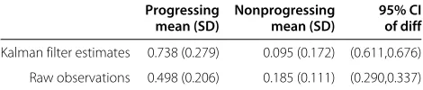
The final logistic regression models are summarized in Additional file 2: Table S2. Both models use the same set of final variables, however the odds ratios are larger for the model trained on Kalman filter estimates than the odds ratios for the model trained on raw observa-tions. For instance, the odds ratio of PSD is 1.344 for the logistic regression model based on Kalman filter esti-mates and 1.107 for the logistic regression model based on raw observations. Analysis of the logistic regression fitted values, i.e. the estimated probability of progres-sion, is presented in Table 1. It is important to note that the average estimated probability of progression of the Kalman filter progressing instances (0.738) is much higher than the average for the raw observations progress-ing instances (0.498). Additionally, the difference between average fitted values of progressing and nonprogressing instances is much greater for the Kalman filter estimates (95% CI 0.611,0.676) than for the raw observations data set (95% CI 0.290,0.337). This increased difference of aver-age fitted values between progressing and nonprogressing instances supports our hypothesis that Kalman filtered estimates allows for improved distinction of significant disease progression.
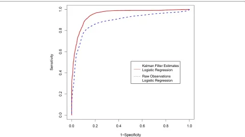
Finally, the ROC curve, Figure 1, illustrates that by first filtering the data using the Kalman filter model, we can achieve higher sensitivity and specificity than a model based on the raw observations. For example, if we select
Table 1 Fitted probabilities from logistic regression models
Progressing Nonprogressing 95% CI
mean (SD) mean (SD) of diff
Kalman filter estimates 0.738 (0.279) 0.095 (0.172) (0.611,0.676)
Raw observations 0.498 (0.206) 0.185 (0.111) (0.290,0.337)
The table provides the mean and standard deviation of the fitted probabilities for progression and nonprogression instances from both logistic regression models.
95% sensitivity as our goal, we can obtain 83% specificity using the Kalman filter model but only 39% specificity using the raw observations model. At 90% sensitivity, the Kalman filter achieves 88% specificity while the raw obser-vations model achieves 66% specificity. The mean (and variance) of the estimated AUC for the Kalman filter and raw observations models are 0.961 (0.002) and 0.889 (0.013), respectively. Hence, using the probability function generated via Kalman filter state estimates and GEE for logistic regression, we are able to more accurately classify patients and instances as experiencing or not experiencing significant OAG progression.
Discussion
Using Kalman filter forecasts in determinations of when patients with OAG should be observed by their physi-cian required the development of a mapping from the filtered health metrics to a probability of progression. The application of GEE for logistic regression on Kalman filtered longitudinal observations of patients with OAG resulted in improved ability to identify significant glau-coma progression as compared to the model generated using the raw clinical trial data. The Kalman filter model is able to better detect relationships between health met-rics and the more complex disease progression definition than the logistic regression model using raw observa-tions as inputs. We believe that as the progression defini-tion becomes more heavily influenced by systematic pro-cess and measurement noise, a logistic regression model parameterized on Kalman filter estimates of the input will become increasingly more beneficial for detecting disease progression.
Kalman Filter Estimates Logistic Regression
Raw Observations Logistic Regression
Figure 1ROC curves for Kalman filter estimates and raw measurements logistic regression models.Estimates of sensitivity and specificity obtained via 10-fold cross validation are used to generate the receiver operating characteristic (ROC) curve for the two logistic regression models parameterized with Kalman filter estimates and raw observations.
mean fitted values creates a larger set of thresholds for which there are fewer false negatives and false positives. The lower rate of false negatives and false positives leads to improved sensitivity and specificity for the Kalman fil-ter model at detecting significant glaucoma progression in comparison to the raw measurements.
The difference of mean fitted values for the Kalman fil-ter model is larger because of the greafil-ter in magnitude covariate coefficients and higher odds ratios of the model covariates. With higher odds ratios, each unit increase in a predictive covariate increases the probability of progres-sion more greatly for the Kalman filter model than it does for the raw measurements model.
The greater in magnitude covariate coefficients and higher odds ratios are explained by the linear system model the Kalman filter uses for state estimation. In the case of glaucoma, IOP decreases over time for treated patients and mean deviation becomes more negative since VF loss cannot be reversed. The trend creates the larger difference in mean variable values as the num-ber of measurements increases. The “noisy” nature of the raw measurements creates fluctuation around this expected trend. Because the GEE approach is concerned with population-averaged (i.e. the mean response) vari-able, we expect covariate coefficients to be greater in magnitude when the difference between the mean
vari-able value for progression and nonprogression instances increases.
The increased standard deviation of the mean value of the Kalman filter estimates is due to the Kalman filter’s recognizing each patient’s individual disease realization. As the Kalman filter updates the state estimates to reflect a patient’s particular characteristics, that patient’s trajec-tory becomes more dissimilar to the trajectories of other patients. The “noisy” raw measurements mask these dis-similar trajectories which results in clustered mean vari-able values for progressing or nonprogressing instances.
Increased sensitivity and specificity of classification models improves clinical decision making by more accurately identifying significant disease progression. Clinicians who are able to correctly identify patients who experience significant glaucoma progression can make more informed decisions, such as improving mon-itoring schedules and improving treatment decisions. Additionally, the increased accuracy allows clinicians to utilize the statistical model without fearing high rates of misclassification.
small, the disease progression mechanics can potentially be estimated by a linear dynamics model. The Kalman filter also assumes the state estimates, noise and raw observations come from a Gaussian distribution. This assumption is reasonable within a range around the mean (2 standard deviations) for bounded variables, e.g. IOP.
The application of our methodology to CIGTS data is limited by the fact that this trial took place between 1993 and 2003. Since 2003, there have been many advances in the field of diagnostic testing for glaucoma including testing to check for damage to the retinal nerve fiber layer tissue using optical coherence tomography (OCT) and additional progression detection software on the visual field machines such as Guided Progression Analy-sis (GPA). In the future, we plan to use data from other sources to be able to integrate data from OCT and GPA into our models and progression definition.
Conclusion
In this paper, we applied a linear system dynamics model approach, using a Kalman filter, to estimate true measure-ment values for variables which have both measuremeasure-ment and process noise. Filtering techniques are important for true measurement estimation for medical decision making and have been shown to result in improved significant disease progression classification when utiliz-ing GEE for logistic regression with repeated measures data, as demonstrated in our modeling of OAG pro-gression dynamics. Due to process and measurement noise, only after having seen future observations can clin-icians retrospectively assess whether “true” progression has occurred. Logistic regression models that directly consider those noises allow for the prospective calculation of the probability of experiencing progression. Further-more, for complex progression definitions, logistic regres-sion enables a reduction in the number of variables to consider, which is important in guiding clinical decisions. This methodology is also applicable to other chronic dis-eases, particularly those diseases whose dynamics can be modeled effectively by a linear system and whose biomarkers can be reasonably approximated by a Gaussian distribution.
Additional files
Additional file 1: Summary of Kalman filter estimates and raw observations.The table provides the overall mean and standard deviation for the variables at progressing and nonprogressing instances. Kalman filter estimates and raw observations of these variables are compared. Additional file 2: Coefficients of logistic regression.The table presents the final covariate sets for the two logistic regression models
parameterized with Kalman filter estimates and raw observations. We present the mean (variance) of the coefficient parameters of the iterations of the 10-fold cross validation.
Competing interests
All authors currently have a provisional patent and have filed a patent application (“Patient-Specific Modeling and Forecasting of Disease Progression”, Atty. Docket No. 010109-11001A) related to the content of this manuscript.
Authors’ contributions
GS prepared the manuscript, assisted in the design of the study, and performed the computational analysis. ML conceived and supervised the research, provided intellectual guidance, and revised the manuscript. JS provided subject matter expertise, supervised analysis, and revised the manuscript. DM provided the clinical trial data and subject matter expertise. All authors read and approved the final manuscript.
Acknowledgements
The authors would like to acknowledge the contributions of Jonathan Helm, Mark Van Oyen, and Leslie Niziol to the work presented.
Author details
1Department of Industrial and Operations Engineering, University of Michigan,
Ann Arbor, Michigan, USA.2Department of Ophthalmology and Visual
Sciences, University of Michigan, Ann Arbor, Michigan, USA.
Received: 22 February 2013 Accepted: 13 December 2013 Published: 21 December 2013
References
1. Friedman D, Wolfs R, O’colmain B, Klein B, Taylor H, West S, Leske M, Mitchell P, Congdon N, Kempen J:Prevalence of open-angle glaucoma among adults in the United States.Arch Ophthalmol2004,122(4):532. 2. Quigley H, Broman A:The number of people with glaucoma
worldwide in 2010 and 2020.Br J Ophthalmol2006,90(3):262–267. 3. Lee P, Walt J, Rosenblatt L, Siegartel L, Stern L:Association between
intraocular pressure variation and glaucoma progression: data from a United States chart review.Am J Opthalmol2007,144(6):901–907. 4. Musch D, Gillespie B, Niziol L, Cashwell L, Lichter P:Factors associated
with intraocular pressure before and during 9 years of treatment in the collaborative initial glaucoma treatment study.Ophthalmology 2008,115(6):927–933.
5. Bengtsson B, Patella V, Heijl A:Prediction of glaucomatous visual field loss by extrapolation of linear trends.Arch Ophthalmol2009, 127(12):1610.
6. Diaz-Aleman V, Anton A, de la Rosa M, Johnson Z, McLeod S,
Azuara-Blanco A:Detection of visual-field deterioration by glaucoma progression analysis and threshold noiseless trend programs.Br J Ophthalmol2009,93(3):322.
7. McNaught A, Hitchings R, Crabb D, Fitzke F:Modelling series of visual fields to detect progression in normal-tension glaucoma.Graefe’s Arch Clin Exp Ophthalmol1995,233(12):750–755.
8. Zahari M, Mukesh B, Rait J, Taylor H, McCarty C:Progression of visual field loss in open angle glaucoma in the melbourne visual impairment project.Clin Exp Ophthalmol2006,34:20–26. 9. Lenert L, Sturley A, Rupnow M:Toward improved methods for
measurement of utility: automated repair of errors in elicitations.
Med Decis Making2003,23:67.
10. Marshall T:Misleading measurements: modeling the effects of blood pressure misclassification in a United States population.Med Decis Making2006,26(6):624.
11. Brovko O, Wiberg D, Arena L, Bellville J:The extended Kalman filter as a pulmonary blood flow estim [combining dot above] ator.
Automatica1981,17:213–220.
12. McNames J, Aboy M:Statistical modeling of cardiovascular signals and parameter estimation based on the extended Kalman filter.
Biomed Eng IEEE Trans2008,55:119–129.
13. Kuure-Kinsey M, Palerm C, Bequette B:A dual-rate Kalman filter for continuous glucose monitoring.InProceedings of IEEE for Engineering in Medicine and Biology Society: 30 Aug-3 Sept 2006Edited by IEEE. New York, NY: IEEE; 2006:63–66.
15. Roshanov P, Gerstein H, Hunt D, Sebaldt R, Haynes R:Impact of a computerized system for evidence-based diabetes care on completeness of records: a before–after study.BMC Med Inform Decis Making2012,12:63.
16. Silverman E, Chapman H, Drazen J, Weiss S, Rosner B, Campbell E, O’Donnell W, Reilly J, Ginns L, Mentzer S, et al.:Genetic epidemiology of severe, early-onset chronic obstructive pulmonary disease. Risk to relatives for airflow obstruction and chronic bronchitis.Am J Respir Crit Care Med1998,157(6):1770.
17. Doebbeling B, Edmond M, Davis C, Woodin J, Zeitler R:Influenza vaccination of health care workers: evaluation of factors that are important in acceptance* 1.Prev Med1997,26:68–77.
18. Albert P, McShane L:A generalized estimating equations approach for spatially correlated binary data: applications to the analysis of neuroimaging data.Biometrics1995,51(2):627–638.
19. Hodapp E, Parrish II R, Anderson D, Perkins T:Clinical decisions in glaucoma. St. Louis, MO: Mosby; 1993.
20. Nouri-Mahdavi K, Caprioli J, Coleman A, Hoffman D, Gaasterland D: Pointwise linear regression for evaluation of visual field outcomes and comparison with the advanced glaucoma intervention study methods.Arch Ophthalmol2005,123(2):193.
21. Kalman R:A new approach to linear filtering and prediction problems.J Basic Eng1960,82:35–45.
22. Shumway R, Stoffer D:An approach to time series smoothing and forecasting using the EM algorithm.J Time Ser Anal1982,3(4):253–64. 23. Zeger S, Liang K, Albert P:Models for longitudinal data: a generalized
estimating equation approach.Biometrics1988,44(4):1049–1060. 24. Halekoh U, Højsgaard S, Yan J:The R package geepack for generalized
estimating equations.J Stat Softw2006,15(2):1–11.
doi:10.1186/1472-6947-13-137
Cite this article as: Schellet al.:Filtering data from the collaborative initial glaucoma treatment study for improved identification of glaucoma progression.BMC Medical Informatics and Decision Making201313:137.
Submit your next manuscript to BioMed Central and take full advantage of:
• Convenient online submission
• Thorough peer review
• No space constraints or color figure charges
• Immediate publication on acceptance
• Inclusion in PubMed, CAS, Scopus and Google Scholar
• Research which is freely available for redistribution