SIMULATION STUDIES ON AUTOMATIC GENERATION CONTROL IN DEREGULATED ENVIRONMENT WITHOUT CONSIDERING GRC

(1)

SIMULATION STUDIES ON

AUTOMATIC GENERATION CONTROL

IN DEREGULATED ENVIRONMENT

WITHOUT CONSIDERING GRC

A. Suresh Babu,

Assoc.Prof., Dept. of EEE, SSNEC,Ongole,A.P., INDIA

[email protected]

Prof. Ch.Saibabu,

Director-Admissions, JNTUK, Kakinada, AP, INDIA

[email protected]

Abstract— In this paper, analysis of automatic generation control (AGC) using integral controller is carried out in the deregulated environment. The traditional AGC of two area system is modified and implemented in deregulated environment to account the effect of contracted and un-contracted power demands on system dynamics. The concept of DISCO participation matrix (DPM) to simulate bilateral contracts is proposed. Gain setting of integral controller is optimized without considering Generation Rate Constraint (GRC) using Integral Squared Error (ISE) technique.

Key words – Automatic generation control, deregulation, optimization, DISCO participation matrix, Integral Squared Error

I. INTRODUCTION

The net power flow on the tie lines connecting a system to the external system is frequently scheduled by an a priori contract basis. System disturbances caused by load fluctuations result in changes in tie-line power and system frequency which give rise to a Automatic Generation Control (AGC) problem.

The AGC is based on an error signal called Area Control Error (ACE) which is a linear combination of net-interchange and frequency errors. The conventional control strategy used in industry is to take the integral of ACE as the control signal [1-4]. It has been found [2] that the use of ACE as the control signal reduces the frequency and tie-line power error to zero in the steady state. The main objective is to find optimum gain value of I- controller. Trajectory sensitivities were used to obtain optimal parameter of system using gradient Newton algorithm [7].

II. RESTRUCTURED POWER SYSTEM

The electric supply industry in nearly every country for a major part of the last century was a natural monopoly and being so; it attracted regulation by the government. Without exception, the industry was a vertically integrated regulated monopoly that owned the generation, transmission and distribution facilities. It was also a local monopoly, in the sense, that in any area one company or government agency sold electric power and services to all consumers.

(2)

Fig 1: Vertically integrated utility structure

The VIU is usually interconnected to other VIUs through the tie-lines. This interconnection permits the buying and selling of power between the VIUs along the tie lines and also provides greater reliability. The VIU is responsible for maintaining the physical flow of electricity, satisfying consumer’s demands of proper voltage and frequency level, maintaining security, economy and reliability of the system, settling the electricity bills with the customers, ensuring proper control, protection, and all such measures for the proper functioning of the system.

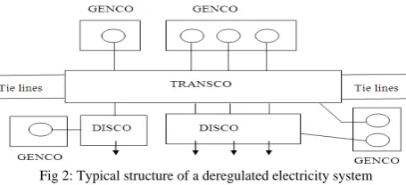
Since 1980’s, the electricity supply industry has been undergoing rapid and irreversible changes thereby reshaping an industry hat for a long time has been remarkably stable and has served the public well. An important feature of these changes is to allow for competition among generating utilities and to create market conditions in the sector which are seen as necessary for reducing the cost of energy production and distribution, eliminate certain inefficiencies and offer increased choice to the customer. This transition towards a competitive power market is commonly referred to as restructuring of the electricity supply industry or deregulation. With the restructuring of the electricity supply industry new companies emerged, namely, generation companies (GENCOs), transmission companies (TRANSCOs), distribution companies (DISCOs) and independent contract administrator (ICA). A typical structure a deregulated electricity system is shown in Fig 2.

Fig 2: Typical structure of a deregulated electricity system

The GENCOs compete in a free market to sell the electricity they produce. The retail customer buys the electricity from the DISCOs and the responsibility for the transfer of the power from the GENCOs to the DISCOs is that of the TRANSCO. Although only one TRANSCO has been shown in the Fig, in reality there may be more than one TRANSCO and these TRANSCOs will continue to be interconnected. Thus a bilateral transaction of power between a GENCO and a DISCO may flow through more than one TRANSCO.

The major difference between a conventional monopolistic electricity market and the emerging deregulated competitive market is that electricity in the former case is considered merely as energy supply sector, whereas in the latter case it is treated as a service sector and so is marketed as any other commodity. Power system deregulation is expected to offer the benefits of lower electricity price through competition, better consumer service and improved system efficiency. However, it throws several technical challenges with respect to its conceptualization and integrated operation. Basic issues of ensuring economics, secure and stable operation of the power system, while delivering power at desired quality in terms of voltage and frequency magnitude, have to be addressed carefully in the deregulated market which is likely to become more complex as compared to the present regulated monopolistic system.

In the conventional market, a single utility is responsible for maintain the physical flow of electricity, satisfying consumer’s demands of proper voltage and frequency level, maintaining security, economy and reliability of the system, setting the electricity bills with the customers, ensuring proper control, protection, and all such measures for the proper functioning of the system.

(3)

Objectives:

Main objectives of the present work are

1. To optimize the gain setting of integral controller in continuous mode of two area interconnected power system by using integral squared error (ISE) technique.

3. To study the AGC problem in deregulated environment for various scenarios.

III. MATHEMATICAL MODELLING OF AGC IN DEREGULATED ENVIRONMENT

a) Disco participation matrix

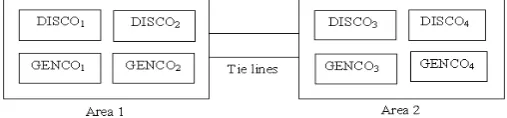
In the deregulated environment, GENCOs sell power to various DISCOs at competitive prices. As there are several GENCOs and DISCOs in the deregulated structures, a DISCO has the freedom to have a contract with any GENCOs in their own control areas. A DISCO may also have a contract with a GENCO in another control area. This makes various combinations of GENCO-DISCO contracts possible in practice. The “DISCO participation matrix” (DPM) makes the visualization of these contracts easier. DPM is a matrix with the number of rows equal to the number of generating units and the number of columns equal to the number of DISCOs in the system. Each entry in this matrix can be thought of as a fraction of its total load contracted by a DISCO (column) towards a generating unit (row). Thus the ‘ij’th element of the matrix corresponds to the fraction of its total load contracted by DISCO ‘j’ from generating unit ‘i’. The sum of all the entries in a particular column, corresponding to a DISCO which demands power, in this matrix is unity. If the column corresponds to a DISCO which does not demand any contracted power then all the entries in that column are zero. The DPM shows the participation of a DISCO in a contract with a generating unit, hence the name “DISCO participation matrix”. Consider a two-area system in which each area has two GENCOs and two DISCOs in it. Each of the GENCO has only one generating unit under it: Let GENCO1, GENCO2, DISCO1 and DISCO2 be in Area 1 and GENCO3,

GENCO4, DISCO3 and DISCO4 be in Area 2as shown in Fig 3.

Fig 3. Schematic of a two-area system in a deregulated environment

The DPM for this system is

DPM

=

cpf cpf cpf cpf

---(1)

Where ‘cpf’ refers to “contract participation factor”. As mentioned earlier the sum of all the entries in a column in the DPM is unity, if the column corresponds to a DISCO which demands contracted power, i.e,

∑ cpfij = 1 for i = 1 to 4 ( total number of GENCOs )

The block diagonal of DPM corresponds to local demands while the off diagonal block corresponds to the demand of DISCOs in one area with the GENCOs in another area.

To illustrate the concept, suppose that DISCO2 demands 0.04 pu power, out of which, 0.01 pu is demanded from GENCO1, 0.012 pu from GENCO2, 0.014 pu from GENCO3 and 0.004 pu from GENCO4. Then

the entries in column 2 of equation (1) are as follows:

cpf12 = 0.01/0.04 = 0.25 cpf22 = 0.012/0.04 = 0.30

cpf32 = 0.014/0.04 = 0.35 cpf42 = 0.004/0.04 = 0.10

b) Block Diagram Formulation

Consider the two area system shown schematically in Fig. 4 Whenever a load demanded by a DISCO changes , it is reflected as a local load in the area to which the DISCO belongs. So if ∆Pli, where i = 1 to 4 (

number of DISCOs ) , denote the total power demanded by DISCOi from various GENCOs as per its contracts

with them, then the local load for a particular control area ‘j’ is given by the following expressions:

∆Plj,loc=∑∆Pli ; where j=1,2

(4)

These local loads should be reflected at the point of input to the power system block. It may also happen that a DISCO violates its contracts by demanding more power than that specified in the contracts. This excess power is not contracted out to any GENCO and this un-contracted power demand must be supplied by the GENCOs in the same area as the concerned DISCO. It must be reflected as a local load of the area but not as the contracted demand, which is also shown at the point of input to the power system block (Fig .4). As in the case of contracted power demands, if ∆Pi,uc, where i= 1 to 4 ( number of DISCOs ) , denotes the un-contracted

power demanded by DISCOi, then the un-contracted power demand for a particular control area ‘j’ is given by

the following expression:

∆Plj,uc=∑∆Pi,uc ; where j=1,2

i = 1, 2 for j=1 --- (3)

= 3, 4 for j=2 As there are many GENCOs in each area, ACE signal has to be distributed among them in proportion to their participation in AGC. Coefficients that distribute ACE to several GENCOs are termed as “ ACE participation factors” (apfs). apfij represents the ACE participation factor of GENCO ‘i’ in area ‘j’, also, the sum of all the apfs in an area is unity. In the deregulated environment a DISCO asks/demands a particular GENCO or units for power. These demands must be reflected in the dynamics of the system. Turbine and governor units must respond to this power demand. Thus, as a particular set of GENCOs are supposed to follow the load demanded by a DISCO, information signals must flow from a particular DISCO to a particular GENCO specifying corresponding demands. The demands are specified by cpfs and the pu load of a DISCO. These signals carry information as to which GENCO has to follow a load demanded by which DISCO. The scheduled steady state power flow on the tie line is given as: ∆Ptie12, scheduled = (Demand of DISCOs in Area 2 from GENCOs in Area 1) – (Demand of DISCOs in Area 1 from GENCOs in Area 2) 2 4 4 2 1 3 3 1 ij ij ij ij i j i j

cpf

P



cpf

P

   



 

--- (4)

The tie line power error, ∆Ptie12, scheduled, is defined as:

∆

Ptie12,error=

∆

Ptie12, actual-

∆

Ptie12,scheduled ---- (5)

At the steady state, the tie line power error, ∆Ptie12, error vanishes as the actual tie line power flow reaches the scheduled power flow. This error signal is used to generatethe respective ACE signals as in the traditional scenario ACE1 = B1 ∆f1 + ∆Ptie12, error ACE2=B2∆f2+a12∆Ptie12,error --- (6)

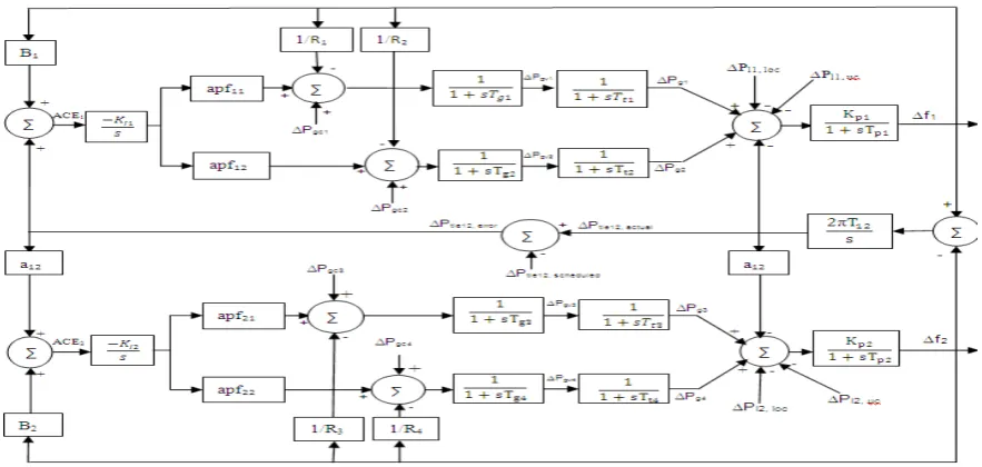
where a12 = - (Pr1/Pr2) with Pr1, Pr2 being the rated powers of areas 1 and 2 respectively. Keeping in view the above, the block diagram from AGC in a deregulated system, as per the model described in this section, is shown in Fig 4. c).State space representation The dynamic model of the system shown in Fig .4 can be written as: X AX BU Гp γp/

_----(7)

where X and U are the state and control vectors respectively and p and p/ are the disturbance vectors. X = [∆f1∆f2 ∆Ptie12,actual∆Pg1∆Pg2 ∆Pg3 ∆Pg4∆Pgv1∆Pgv2 ∆Pgv3 ∆Pgv4]T

----(8)

U=[u1u2]T

----(9)

p=[∆Pl1∆Pl2∆Pl3∆Pl4]T

---(10)

p

/

=[

∆

Pl1,uc

∆

Pl2,uc]

T

---(11)

The control signals of areas 1 and 2 are given as: u1=-KI1∫ACE1dt

---(12)

u2=-KI2∫ACE2dt

---(13)

KI1 and KI2 are the gains of the AGC controllers.

(5)

Fig 4: Block diagram of two area system with two units per area

d). Optimization of controller gain

Optimization of gain setting is based on the Integral Squared Error (ISE) criteria where the objective is to minimize the objective function J given by,

J = Δf12 + Δf22 + a12 ΔPtie2 )*dt ---(14)

For getting the optimum value of integral gain, the values of objective function ‘J’are obtained for a set of Ki values with a step load disturbance of 1% in area one.

Fig. 5 show the plot of J vs Ki without considering GRC.

Fig.5. Ki vs J for two interconnected area power system (with GRC)

The optimized value of controller gain Ki= 0.65.

IV. SIMULATION RESULTS: TWO AREA SYSTEM WITH TWO GENERATING UNITS PER AREA.

To illustrate the behavior of the AGC scheme being described, a two area system as given in Figs 3 and 4 is used. The two control areas are assumed to be identical. Also the governor-turbine units in each area are assumed to be identical.

Case 1: Base case:-Assume that the GENCOs in each area participate equally in AGC, i.e, ACE participation factors are:

apf11= apf12= apf21= apf22=0.5

It is assumed that the load is demanded by DISCO1 and DISCO2 only, and so the load change occurs in Area 1 not in Area 2. Let the value of this load demand be 0.05 pu for each of them. It is also assumed that DISCO1 and DISCO2 demand identically from GENCO1 and GENCO2. There is no un-contracted power

demand. Thus,

∆Pl1 = ∆Pl2 = 0.05 pu ∆Pl3 = ∆Pl4 = 0 pu

∆Pl1,uc = ∆Pl2,uc = 0 pu

and the DPM becomes

OBJ

E

CT

IV

E FUNCT

ION (

J)

(6)

DPM=

0.5 0.5 0 0 0.5 0.5 0 0 0 0 0 0 0 0 0 0

Substituting the above data in equation (4) we get, ∆Ptie12, scheduled = 0 pu

In the steady state, the generation of a generating unit must match the demands of all the DISCOs having contracts with it. The desired generation of each GENCO at the steady state can be expressed as:

∆P ,

cpf cpf cpf cpf cpf cpf cpf cpf cpf cpf cpf cpf cpf cpf cpf cpf

∆P ∆P ∆P ∆P

--- (15)

Substituting the data of this case in equation (15) we get, ∆Pg1,ss = 0.05 pu ∆Pg2,ss = 0.05 pu

∆Pg3,ss = 0.0 pu ∆Pg4,ss = 0.0 pu

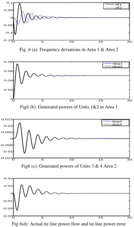
Figs 6(a) to 6(d) show the dynamics responses of the system for the case under consideration: area frequency deviation, generate powers of various GENCOs following a step change in the load demands of DISCO1 and

DISCO2 and the power flow on the tie line, actual and error. The frequency deviation in each area goes to zero

in the steady state [ Fig 6(a) ]. As only the DISCOs in Area 1 have non-zero load demands the transient dip in frequency of Area 1 is larger than that of Area 2. Fig 6(b) shows the responses of GENCO1 and GENCO2, which

are identical while Fig 6(c) shows the responses of GENCO3 and GENCO4, which are identical. The actual

generated powers reach the desired values at the steady state. Fig 6(d) shows that the tie line power at the steady state (∆Ptie12, actual) goes to zero which equals the scheduled value. Also since the scheduled tie line power

(∆Ptie12, scheduled) is zero, the plots for the tie line power flow, actual and error, are identical.

Fig .6 (a): Frequency deviations in Area 1 & Area 2

Fig6 (b): Generated powers of Units 1&2 in Area 1

Fig6 (c): Generated powers of Units 3 & 4 Area 2

Fig 6(d): Actual tie line power flow and tie line power error

0 5 10 15 20

-0.15 -0.1 -0.05 0 0.05 0.1

df1 df2

0 5 10 15 20

0 0.02 0.04 0.06 0.08

dpg1 dpg2

0 5 10 15 20

-0.015 -0.01 -0.005 0 0.005 0.01 0.015

dpg3 dpg4

0 5 10 15 20

(7)

Case 2

: Without contract violation:- In this case, it is assumed that load changes occur in both Area 1 and Area 2. Also the DISCOs have power contracts with the GENCOs, not only in their own area but also in the other area as per the following DPM:

DPM=

0.5 0.25 0 0.3 0.2 0.25 0 0

0 0.25 1 0.7 0.3 0.25 0 0

Each DISCO demands 0.05 pu power from the GENCOs as per the ‘cpfs’ given in the DPM and there is no un-contracted power demand from any of the DISCOs. Therefore,

∆Pl1 = ∆Pl2 = 0.05 pu ∆Pl3 = ∆Pl4 = 0.05 pu

∆Pl1,uc = Un-contracted power demand in Area 1= 0 pu

∆Pl2,uc = Un-contracted power demand in Area 2= 0 pu

All the GENCOs participate in AGC as defined by the following ‘apfs’: apf11= 0.75 apf12= 0.25

apf21= 0.50 apf22= 0.50

The ACE participation factors affect only the transient behavior of the system and not the steady state behavior when un-contracted power demands are absent.

Substituting the above mentioned data in equation (4) we get,

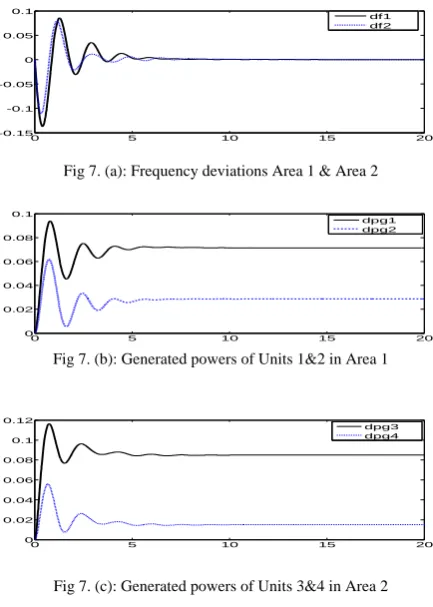
∆Ptie12, scheduled = - 0.0125 pu

Also, by substituting the respective data of this case in equation (15) we get,

∆Pg1,ss = 0.0525 pu ∆Pg2,ss = 0.0225 pu

∆Pg3,ss = 0.0975 pu ∆Pg4,ss = 0.0275 pu

Figs 7(a) to 7(d) show the dynamic responses of the system for the case under consideration

.

Fig 7. (a): Frequency deviations Area 1 & Area 2

Fig 7. (b): Generated powers of Units 1&2 in Area 1

Fig 7. (c): Generated powers of Units 3&4 in Area 2

0 5 10 15 20

-0.15 -0.1 -0.05 0 0.05 0.1

df1 df2

0 5 10 15 20

0 0.02 0.04 0.06 0.08 0.1

dpg1 dpg2

0 5 10 15 20

0 0.02 0.04 0.06 0.08 0.1 0.12

(8)

Fig 7 (d): Actual tie line power flow and tie line power error

Case 3

:With contract violation:- If a DISCO demands more power than what is specified in its contracts with various units, then the excess power is not contracted out to any GENCO. This un-contracted power must be supplied by the units in the same area as the DISCO, which has violated its contracts by demanding excess power. Let us consider Case 2, again with a modification that DISCO1 demands 0.05 pu of excess power. Rest

all remains same as in Case 2. So here

∆Pl1,uc = Un-contracted power demand in Area 1 = 0.05 pu

∆Pl2,uc = Un-contracted power demand in Area 2 = 0 pu

With the presence of un-contracted demand the generation of the units at steady state does not equal their contracted values (as given by matrix equation (15)) but is given by the following matrix equation:

∆P , ∆P , ∆P , ∆P ,

cpf cpf cpf cpf

∆P ∆P ∆P ∆P

∆P , 0 0 0

0 ∆P , 0 0

0 0 ∆P , 0

0 0 0 ∆P,

apf apf apf apf

--- (16)

From the above equation it can be seen that the ACE participation factors decide the distribution of any un-contracted load in the steady state.

Substituting the data of the case under consideration in the equation (15) we get,

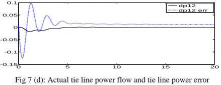
∆Pg1,ss = 0.09 pu ∆Pg2,ss = 0.035 pu

∆Pg3,ss = 0.0975 pu ∆Pg4,ss = 0.0275 pu

Also from equation (4), for this case, we get, ∆Ptie12, scheduled = - 0.0125 pu

Figs. 8(a) to 8(d) show the dynamics responses of the system for the case under consideration. The frequency deviation in each area goes to zero in the steady state [Fig. 8(a)]. Fig 8(b) and 8(c) show the responses of GENCO1

,

GENCO2 and GENCO3, GENCO4 respectively. The steady state generations of GENCO3 and

GENCO4 arenot affected by the excess load of DISCO1. The un-contracted load of DISCO1 is reflected in the

generation of GENCO1 and GENCO2. Thus, this excess load is taken up by the units in the same area as that of

the DISCO making the un-contracted demand. Fig 8(d) shows that the tie line power at the steady state goes (∆Ptie12, actual) to the scheduled value.

Fig 8 (a): Frequency deviations Area 1 & Area 2

Fig 8 (b): Generated powers of Units 1&2 in Area 1

0 5 10 15 20

-0.15 -0.1 -0.05 0 0.05 0.1 dp12 dp12 err

0 5 10 15 20 25 30

-0.2 -0.15 -0.1 -0.05 0 0.05 df1 df2

0 5 10 15 20

(9)

Fig 8 (c): Generated powers of Units 3&4 in Area 2

Fig 8(d): Actual tie line power flow and tie line power error

V. CONCLUSION

The role and importance of AGC in deregulated environment are investigated with necessary modifications. The contracted power is given as an input directly to the governor of GENCO. From the simulation of various cases, it has been observed that ACE participation factors affect only the transient behavior of the system and not the steady state when there are no un-contracted loads. However, if un-contracted power demand is present, the ACE participation factors decide the distribution of the un-contracted load in the steady state. Thus, this excess load is taken by the units in the same area as that of DISCOs making the excess demand. With this model even if there is an un-contracted power demand in the system, the frequency deviation goes to zero and the actual tie line power flow settles to the scheduled value in the steady state. Using ISE without considering GRC optimum value of controller gain is obtained.

VI. REFERENCES

[1] C.W.ROSS, 'Error adaptive control of interconnected power systems', IEEE Trans., PAS-85, pp. 742-749, 1966.

[2] O.I. ELGERD and C.E.FOSHA, 'Optimum megawatt frequency control of multi-area electric energy system', IEEE Trans., PAS-89,

pp. 556-563, 1970.

[3] J. NANDA and B.L.KAUL, 'Automatic generation control of an interconnected power system', Proc. IEE, 125, (5), pp. 385-390, 1978.

[4] R. Christie and A. Bose, “Load-frequency control issues in power systems operations after deregulation” IEEE Trans. Power systems, vol. 11, no. 3, pp 1191-1200, Aug 1996.

[5] J. Kumar K. Ng and G. Sheble, “AGC simulator for price-based operation: Part-1” IEEE Trans. Power Systems, vol. 12, no. 2, pp 527-532, May 1997.

[6] E. Nobile, A. Bose and K. Tomsovic, “Feasibility of a bilateral market for load following” IEEE Trans. Power Systems, vol. 16, no. 4, pp 782-787, Nov 2001.

[7] V. Donde, M.A. Pai and I.A. Hiskens, “Simulation and optimization in an AGC system after deregulation”, IEEE Trans. Power systems, vol. 16, no. 3, pp 481-489, Aug 2002.

[8] B.H. Bakken and O.S. Grande, “Automatic Generation Control in a deregulated power system”, IEEE Trans. Power systems, vol. 13, no. 4, pp 1401-1406, Nov 1998.

Appendix

1. The order of A matrix is (11 11) and the non-zero elements of the matrix are given below:

A(1,1) = (-1/Tg1) A(1,3) = (-1/R1Tg1)

A(2,1) = (1/Tt1) A(2,2) = (-1/Tp1)

A(3,2) = (Kp1/Tp1) A(3,3) = (-1/Tp1)

A(3,5) = (Kp1/Tp1) A(3,11) = (-Kp1/Tp1)

A(4,3) = (-1/R2Tg2) A(4,4) = (-1/Tg2)

A(5,4) = (1/Tt2) A(5,5) = (-1/Tt2)

A(6,6) = (-1/Tg3) A(6,8) = (-1/R3Tg3)

A(7,6) = (1/Tt3) A(7,7) = (-1/Tt3)

A(8,7) = (Kp2/Tp2) A(8,8) = (-1/Tp2)

A(8,10) = (Kp2/Tt2) A(8,11) =(-Kp2/Tp2*a12)