simulated data sets with known errors
Therese Rieckh1,2and Richard Anthes1
1COSMIC Program Office, University Corporation for Atmospheric Research, Colorado, USA 2Wegener Center for Climate and Global Change, University of Graz, Graz, Austria
Correspondence:Richard Anthes ([email protected]) Received: 9 March 2018 – Discussion started: 12 March 2018
Revised: 25 June 2018 – Accepted: 25 June 2018 – Published: 20 July 2018
Abstract. In this paper we compare two different methods of estimating the error variances of two or more independent data sets. One method, called the “three-cornered hat” (3CH) method, requires three data sets. Another method, which we call the “two-cornered hat” (2CH) method, requires only two data sets. Both methods have been used in previous studies to estimate the error variances associated with a number of physical and geophysical data sets. A key assumption in both methods is that the errors of the data sets are not correlated, although some studies have considered the effect of the par-tial correlation of representativeness errors in two or more of the data sets.
We compare the 3CH and 2CH methods using a simple model to simulate three and two data sets with various error correlations and biases. With this model, we know the ex-act error variances and covariances, which we use to assess the accuracy of the 3CH and 2CH estimates. We examine the sensitivity of the estimated error variances to the degree of error correlation between two of the data sets as well as the sample size. We find that the 3CH method is less sensitive to these factors than the 2CH method and hence is more ac-curate. We also find that biases in one of the data sets has a minimal effect on the 3CH method, but can produce large errors in the 2CH method.
1 Introduction
In atmospheric sciences, observations and models are of-ten combined with the goal of providing accurate and com-plete representations of the current or future state of the atmosphere. Knowing the error characteristics of
observa-tions and models is important to understanding the degree to which atmospheric phenomena of interest are accurately de-scribed and analyzed. Estimating observational and model-ing error characteristics is thus of inherent scientific interest. In addition, knowing the error characteristics is important for practical applications such as data assimilation and numer-ical weather prediction. In many modern data assimilation schemes, observations of a given type are weighted propor-tionally to the inverse of their error variance (e.g., Desroziers and Ivanov, 2001).
There are several somewhat similar methods for estimat-ing the error variances associated with two or more data sets. The “three-cornered hat” (3CH) method and the closely re-lated “triple collocation” (TC) method have been used in physics, oceanography and other scientific disciplines to es-timate the errors associated with three independent data sets. Braun et al. (2001) combined two independent data sets, Global Positioning System (GPS) slant water vapor (SWV) and water vapor radiometer (WVR), to estimate the SWV and WVR errors. In analogy to the 3CH method, we refer to the Braun et al. (2001) method as the “two-cornered hat” (2CH) method. Kuo et al. (2004) and Chen et al. (2011) used the “apparent error” (AE) method, which is a variation of the 2CH method, to estimate the error of radio occultation (RO) observations using the known (or estimated) error variance of a forecast model.
3CH method. Variations and enhancements of the method have been applied to many diverse geophysical data sets. The 3CH method has been used to estimate the stability of GNSS clocks using the measured frequencies from multiple clocks (Ekstrom and Koppang, 2006; Griggs et al., 2014, 2015; Luna et al., 2017). Valty et al. (2013) used the 3CH method to estimate the geophysical load deformation computed from GRACE satellites, GPS vertical displacement measurements, and global general circulation models. O’Carroll et al. (2008) compared three systems to measure sea surface tempera-tures: two different radiometers and in situ observations from buoys. They discuss the assumption of neglecting the error correlations among the three data sets and the effect of rep-resentativeness errors. Anthes and Rieckh (2018) used the 3CH method to estimate the error variances of three observa-tional (two radio occultation retrievals and radiosondes) and two model data sets using various combinations of the five data sets.
The major assumption in all of the above methods is that the errors of the three systems are uncorrelated. Correlations between any or all of the three measurement systems will re-duce the accuracy of the error estimates. Other factors that can reduce the accuracy include widely different errors asso-ciated with the three systems or a small sample size. These factors can lead to negative estimates of error variances, es-pecially when the estimates are close to zero (Gray and Al-lan, 1974; Riley, 2003; Griggs et al., 2014).
Stoffelen (1998) developed a closely related method, termed the TC method, to estimate both errors and linear cal-ibration coefficients of surface winds using three data sets. Stoffelen (1998) discussed the correlation between part of the representativeness errors of two of the data sets and sub-tracted the variance common to the scale of these errors from the estimated error variance of one of the data sets used in his pairwise estimate of error variances. This correction requires an independent estimate of the correlated part of the rep-resentativeness error. All variations of TC methods assume that, apart from the correlated part of the representativeness errors, the errors of the different observation systems are un-correlated.
Variations of Stoffelen’s TC method have been have been widely used in the fields of oceanography and hydromete-orology (e.g., Su et al., 2014; Gruber et al., 2016). Roebel-ing et al. (2012) used the TC method to estimate the errors associated with three ways of measuring precipitation: the Spinning Enhanced Visible and Infrared Imager (SEVIRI), weather radars and ground-based rain gauges.
In this paper we estimate the effect of neglecting the error covariances using two or three simulated data sets for which the true error variances and covariances are known. We de-velop a model to simulate the data sets with random and bias errors using a set of assumed true profiles. We then calculate the true error variance and covariance terms in the simulated data sets and show the impact of neglecting these terms on the estimated error variances.
2 Error estimates using the 2CH and 3CH methods We assume we have three data sets,X,Y andZ, that are all measuring the same physical variable, e.g., specific humidity,
q, at the same location and time.
The error variance of the data setXis defined as VARerr(X)=1
n X
(X−true)2=1
n X
Xerr2 , (1)
where true is the true (but unknown) value ofX(as well as
Y andZ),Xerr =(X−true), andn is the number of sam-ples. As discussed in Anthes and Rieckh (2018), this defini-tion includes bias as well as random errors inX. O’Carroll et al. (2008) provide an excellent discussion of the meaning of “true” in the context of the 3CH method.
The error covariance of the data setsXandY is defined as COVerr(X, Y )=1
n X
(X−true)(Y−true). (2)
In general, the errors ofX,Y andZmay be correlated or not. 2.1 Three-cornered hat method
In the 3CH method, the relationship between the error variances, the mean square (MS) differences of X and
Y (MS(X−Y)), and their error covariances are given by Eqs. (7)–(9) of Anthes and Rieckh (2018):
VARerr(X)= 1
2[MS(X−Y )+MS(X−Z)−MS(Y−Z)] +COVerr(X, Y )+COVerr(X, Z)−COVerr(Y, Z), (3) VARerr(Y )=
1
2[MS(X−Y )+MS(Y−Z)−MS(X−Z)] +COVerr(X, Y )+COVerr(Y, Z)−COVerr(X, Z), (4) VARerr(Z)=
1
2[MS(X−Z)+MS(Y−Z)−MS(X−Y )] +COVerr(X, Z)+COVerr(Y, Z)−COVerr(X, Y ). (5) The last three covariance terms in Eqs. (3)–(5) are un-known for real data sets, unless they are estimated indepen-dently, and are neglected when estimating the error variances of the real data setsX,Y andZ. This assumption is valid for no correlation between the errors of the data sets and a large sample size. The estimated error variances are therefore
VARerr(X)est= 1
2[MS(X−Y )
+MS(X−Z)−MS(Y−Z)], (3a) VARerr(Y )est=
1
2[MS(X−Y )
+MS(Y−Z)−MS(X−Z)], (4a) VARerr(Z)est=
1
2[MS(X−Z)
and
VARerr(Z)=MS(Z)−1
4[MS(X+Z)−MS(X−Z)] −2M(true, Zerr)+COVerr(X, Z)
+M(true, Xerr+Zerr)., (7) where M(X)is the mean value of X. The last three error terms in Eqs. (6) and (7) are unknown for real data sets, unless they are estimated independently, and are neglected when estimating the error variances of the real data sets X
andZ:
VARerr(X)est=MS(X)− 1
4[MS(X+Z)
−MS(X−Z)], (6a) VARerr(Z)est=MS(Z)−
1
4[MS(X+Z)
−MS(X−Z)]. (7a) Equations (6a) and (7a) are equivalent to Eqs. (12) and (13) of Braun et al. (2001).
An alternative form of Eqs. (6a) and (7a) that is used in some studies (e.g., Stoffelen, 1998; Vogelzang et al., 2011) is
VARerr(X)est=MS(X)−M(X·Z), (6b)
VARerr(Z)est=MS(Z)−M(X·Z). (7b)
2.3 Comparison of neglected terms in 3CH and 2CH methods
In the 3CH method, the neglected error terms when computing VARerr(X) with Eq. (3) are COVerr(X, Y) + COVerr(X, Z)−COVerr(Y, Z).
In the 2CH method, the neglected error terms when computing VARerr with Eq. (6) are −2M(true,
Xerr)+COVerr(X, Z)+M(true,Xerr+Zerr).
We note that the neglected error terms in the 2CH method contain terms involving the product of true with errors, un-like in the 3CH method. Because true is typically an order of magnitude greater than the errors, these terms are likely much larger than the neglected terms involving only prod-ucts of errors, as in the 3CH method. We also note that if the errors are random and uncorrelated, all of the error terms
AE Xobs Xfcst.
VARerr(Xobs)=MS(Xobs−Xfcst)−VARerr(Xfcst) +2COVerr(Xobs, Xfcst).
The AE is equivalent to the observation minus background (O−B) statistic used in data assimilation studies. In the AE method, the correlation of errors between the observations and forecasts is assumed negligible and the error variance of the forecast is obtained from an independent estimate.
3 Generation of true data set and three simulated data sets with errors
We first generate a set ofnvertical profiles of a variable, true, which we take as specific humidity from the ERA-Interim reanalysis (ERA) (Dee et al., 2011), normalized by the mean specific humidityq averaged over all samples. We next gen-erate three data setsX,Y andZthat are approximations of true (true plus random errors), where the errors ofXandZ
are correlated to a degree that we can control. For simplic-ity, we assume the errors forY are always uncorrelated with those ofXandZ. This is analogous to a system of three ob-servational systems in which the errors of two of them are correlated, but the errors of the third are not. In this section, only random errors are considered. The effect of bias errors is discussed in Sect. 4.4.2.
We then look at the magnitude of the error terms in the 2CH and 3CH methods with various assumed correlation co-efficients between the errors inX andZ and compare the estimated error variances ofX,Y andZwith their true error variances. Our tests will show the impact of the neglect of the error terms depending on the degree of error correlation betweenXandZ.
The assumed normalized random error model for X is given by
The error model is created based on error estimates of specific humidity from several studies (e.g., Kursinski et al., 1997; Collard and Healy, 2003; von Engeln and Nedoluha, 2005; Wang et al., 2013). For example, Collard and Healy (2003) found that, for tropical conditions, the percentage errors for RO specific humidity varied from approximately 10 % near the surface to about 70 % near 300 hPa. Other stud-ies show the errors varying from about 10 % near the sur-face to 100 % in the upper troposphere (about 200 hPa). In our error model, we specified the SD to roughly approximate the SD of RO or radiosonde (RS) data at Minamidait¯ojima (hereafter Mina), Japan (Anthes and Rieckh, 2018; Rieckh et al., 2018). The assumed SD of normalizedq (percent er-ror) given by Eq. (9) is consistent with the above empirical error estimates. Thus the error model is a reasonable one in terms of its magnitude and increase with height. Since it is intended to show the sensitivity of the 3CH and 2CH meth-ods to varying degrees of correlation between two of the data sets used in the comparison, it is not necessary that the error model be a close replication of any particular observing sys-tem, just that the magnitude of the assumed errors and their vertical distribution be reasonable.
3.1 Calculation of correlated errors
In the calculation of the correlated errors, we first generate the random error profilesXerr,YerrandQerr. All of these er-ror profiles are uncorrelated. In general all three erer-ror profiles
Xerr,Yerr andQerr may have different standard deviations, but for these tests we assume all standard deviations vary ac-cording to Eq. (9) for simplicity. We now generate the error profileZerras a linear combination ofXerrandQerr:
Zerr=
a·Xerr+Qerr
1+a , (10)
whereais a specified constant parameter that determines the degree of correlation betweenZerrandXerr. Ifa=0,Zerr=
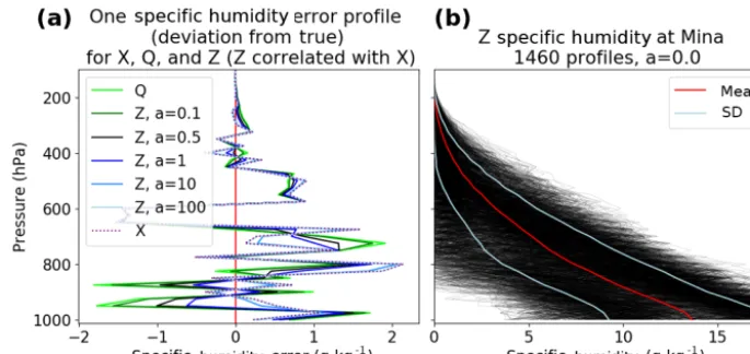
Qerrand the errors ofX,Y andZ are all uncorrelated. Ifa is not equal 0, the errors of Zare correlated with the errors ofX. Figure 1a shows one set of simulated error profiles for the unnormalizedX,Qand severalZfor different values of
a. The transition ofZerrfromQerrtoXerrcan be seen easily between 700 and 800 hPa.Qerr(bright green line) is positive (around 1 g kg−1) andZerrfora=0 is identical to that. For
a=0.1,Zerr has a slightly smaller positive value, andZerr becomes negative as a increases, becoming practically iden-tical withXerr(dotted line) fora=100.
Figure 1b shows the mean and standard deviation for the unnormalized Z specific humidity profiles fora=0. Since
Zerris created by combining the two random errorsQerrand
Xerr, allZerrare overall closer to zero. This will result in a smaller standard deviation ofZif 0< a <∞(especially for values of a close to 1) and will also decrease the true error variance ofZ.
3.2 Relationship of correlation, error variance and error covariance terms
The correlation coefficient r between the Xerr and Zerr is given by
r=1
n
X(Xerr−Xerr)(Zerr−Zerr)
σXerrσZerr
, (11)
whereXerrand Zerrare the mean values of Xerr andZerr, respectively (zero in our error model), andσXerrandσZerrare
the standard deviations ofXerrandZerrgiven by
σXerr =
r 1
n X
X2err≡(VARerr(X))1/2 using Eq.(1), σZerr=
r 1
n X
Zerr2 ≡(VARerr(Z))1/2 using Eq.(1).
The relationship between the correlation coefficient and covariance betweenXerrandZerris therefore
COV(Xerr, Zerr)=rσXerrσZerr≡COVerr(X, Z) using Eq.(2).
It can be shown that for this particular error model
r= a
(1+a2)1/2, (12)
VARerr(Z)=
(1+a2)
(1+a)2VARerr(X), (13)
COVerr(X, Z)=
a
(1+a)VARerr(X). (14)
The correlation betweenXandZerrors can be varied ac-cording to Eq. (12) by varying the parametera, as shown in Table 1. Note that VARerr(Z)≤VARerr(X)and that the max-imum difference between VARerr(X)and VARerr(Z)occurs fora=1 when VARerr(Z)=0.5 VARerr(X)(σZerr =0.707 σXerr).
3.3 Summary of generation of true data set and simulated data sets with random and systematic errors
– We use 2007 ERA specific humidityqprofiles for a lo-cation near Mina, Japan, which is located on Okinawa at 25.6◦N, 131.5◦W. There are four model data profiles per day orn=1460 profiles.
– Assume each vertical profile ofq has no error, and nor-malize theqat each level by the sample mean (q) at that level. This is the “true” data set.
– Generate three different and independent random error profilesXerr,YerrandQerrfrom Eqs. (8) and (9). – GenerateZerrfor various specified values ofato control
Figure 1. (a)One set of error profiles with the unnormalizedXerr(dotted line),Qerr(solid lime green line) andZerr(various solid lines for different values of correlation parametera).Qerris uncorrelated withXerr. Fora= 0,Zerr=QerrandZerrandXerrare uncorrelated. Asa increases,Zerris increasingly correlated withXerrand looks less likeQerrand more likeXerr. For very largea(a= 100),Zerr(light blue solid line) is almost equal toXerr(dotted line).(b)1460 profiles of the unnormalized data setZwith zero correlation withX(a=0).
Table 1.Relationship between normalized error variances and standard deviations of data setsXandZfor different values ofa.
a r σZerr/σXerr VARerr(Z)(%
2) COVerr(X, Z)(%2) 0.0 0.0 1.0 1.00 VARerr(X) 0.0 0.1 0.0995 0.9136 0.84 VARerr(X) 0.0909 VARerr(X) 0.3 0.287 0.803 0.65 VARerr(X) 0.230 VARerr(X) 0.5 0.447 0.745 0.55 VARerr(X) 0.333 VARerr(X) 1.0 0.707 0.707 0.50 VARerr(X) 0.500 VARerr(X) 2.0 0.894 0.745 0.55 VARerr(X) 0.666 VARerr(X) 10.0 0.995 0.913 0.83 VARerr(X) 0.908 VARerr(X) 100.0 0.99995 0.9901 0.98 VARerr(X) 0.990 VARerr(X)
∞ 1.0 1.0 1.00 VARerr(X) 1.0 VARerr(X)
– AddXerr,YerrandZerrto true to obtainX,Y andZ, the 1460 simulated normalized profiles ofq.
– Compute the normalized estimated error variance pro-files of X, Y and Z for the 3CH and 2CH methods according to Eqs. (3a)–(7a) (which have neglected all COV terms) and compare with the true error variances, which can be computed exactly from the full Eqs. (3)– (7) including the known values of the covariance terms. A value ofa=0 should give the most accurate estima-tion of error variances because all covariance terms will be close to zero (they will not be exactly zero because the sample sizenis finite).
4 Effect of error correlations on estimated error variances
We now derive expressions for the estimated values of the error variances forX,Y andZfor this error model and show how the correlations betweenXerrandZerraffect the approx-imate values using the 3CH and 2CH methods. This will give
some insight into how correlations between actual observed data sets will affect estimates of their error variances and standard deviations. To make results more readily compara-ble to previous studies, instead of showing the error variance, we show the square root of the error variance, or the error standard deviation, in most figures.
4.1 Effect of error correlations on 3CH method
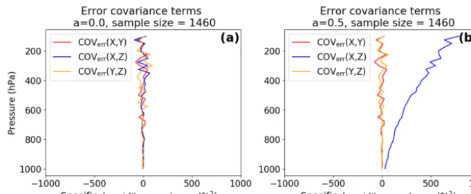
In the 3CH method, three covariance terms are neglected. These terms are zero for an infinite sample size for uncorre-lated errors between the data sets. Correlation between the errors of two data sets will lead to a non-zero covariance term, which becomes larger for larger correlations. The error covariances COVerr(X, Z), COVerr(X, Y )and COVerr(Y, Z) are shown in Fig. 2 fora=0 and 0.5. Note that all error covariances oscillate around zero (and are zero for an in-finitely large sample size) fora=0 (Fig. 2a). Fora=0.5, the COVerr(X, Z)term increases with decreasing pressure, reaching a magnitude of about 800 %2at 100 hPa (Fig. 2b).
ne-Figure 2.Vertical profiles of normalized error covariances (X, Y), (Y, Z) and (X, Z) for(a)a=0 and(b)a=0.5.
glected term in Eq. (3a). Therefore Eq. (3a) can also be ex-pressed as
VARerr(X)est=VARerr(X)−COVerr(X, Z). (2b)
Using Eq. (14) for this error model yields
VARerr(X)est= [1/(1+a)]VARerr(X). (2c) Hence fora >0 the estimated error variance ofX is al-ways less than the true value, as seen in Fig. 3a.
We next consider the effect of theX andZerror correla-tion on the estimate forYerror variance. For our error model, Eq. (4a) can be expressed as
VARerr(Y )est=VARerr(Y )+COVerr(X, Z). (3b) Substituting for the COV term from Eq. (14) and noting that, for our error model, VARerr(X)=VARerr(Y )we obtain VARerr(Y )est= [(1+2a)/(1+a)]VARerr(Y ). (3c) Thus the estimated error variance forY is always greater that the true value fora >0, which is seen in Fig. 3b.
Lastly, we consider the effect of theXandZcorrelation on the estimate for theZ error variance. Equation (5a) can be expressed as
VARerr(Z)est=VARerr(Z)−COVerr(X, Z). (4b)
Substituting for the COV term from Eq. (14) and using Eq. (13) we obtain
VARerr(Z)est= [(1−a)/(1+a2)]VARerr(Z), (4c) so that the estimated error variance forZis less than the true value fora >0, which is illustrated in Fig. 3c. Finally, for
a >1, Eq. (4c) shows that the estimated error variance ofZ
is negative and the SD is undefined. For a=1.0, the esti-mated error variance ofZis zero for an infinite data set, but oscillates around zero because of our finite data set. Thus the estimated SD ofZerris undefined at some levels (Fig. 3c).
4.2 Summary of error correlations on 3CH method For the 3CH method, correlation between the data setsXand
Zhas the following affect on their computed error variances (when covariance terms are neglected):
– VARerr(X)est<VARerr(X)true, – VARerr(Y )est>VARerr(Y )true, – VARerr(Z)est<VARerr(Z)true.
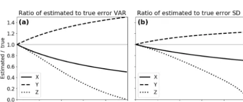
Figure 4 shows the ratios of the approximate error vari-ances and standard deviations to the true values for a ranging from 0 to 1 for the 3CH method. As the correlation parameter
aincreases from 0, the differences between the estimated and true error variances increase. For a modest value ofa=0.2 (correlation coefficient betweenX and Z errors of 0.196), the errors in the SD estimates are−9 % forX,+8 % forY
and−12 % forZ. As the correlation between theX andZ
error reach 0.5, the percentage errors for theX,Y andZ es-timates reach−18,+14.5 and −37 %, respectively. To the extent that this error model gives an idea of the effect of the correlation between the errors of two of the three data sets, estimates of error standard deviations using a large sample of real data should be accurate to within approximately 10 % for correlation coefficients between data errors of 0.2 or be-low, and within 25 % for correlation coefficients of around 0.3. The effect of the correlation betweenZandXerrors on the estimated error variance is greatest on the estimatedZ
error variance.
4.3 Effect of error correlations on 2CH method
We next examine how error correlations in our error model affect the 2CH method. To estimate the error variance of
Figure 3. (a)Estimated standard deviation ofXerrfor values ofa=0, 0.3, 0.5, 1.0 and 100 computed from Eqs. (3a)–(5a). Exact SD computed from data setX(solid black profile).(b)Same as(a)except for estimated SD ofYerr.(c)Same as(a)except for estimated SD of Zerr. Note that for different values ofa, the exact SD ofXerrandYerrare always the same. The exact SD ofZerrdecreases asaincreases for 0< a <1.0. Fora >1.0, the exact SD ofZerrincreases asaincreases, becoming equal to the SD ofXerrfora= ∞due to the way our error model is defined (see also Table 1). Fora=100 the correlation betweenXandZerrors is 0.99995 (Table 1; black dotted line fora=100 almost identical to black solid line fora=0).
Figure 4.Ratio of estimated(a)error variances to true variances and(b)estimated SD to true SD for the 3CH method for values of error correlation parameter a ranging from 0 to 1.0.
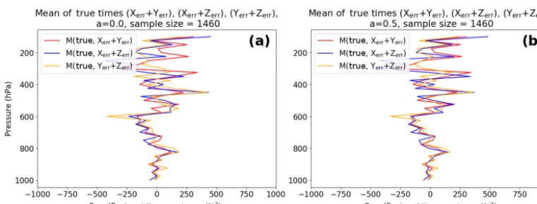
with true, so the non-zero values in Figs. 5–6 are a result of the finite data set (1460 in this example). The COVerr(X, Z) (Fig. 2) increases asaincreases, reaching a maximum value in the upper troposphere of about 800 %2for a=0.5. The terms involving true and the errors inX,Y andZin Figs. 5 and 6 do not change in magnitude with an increasing value ofa, but they increase in amplitude with height and are sig-nificantly large (∼300 %2) compared to the COVerr(X, Z). These results indicate that a large sample size is especially important in the 2CH method, even with a sample size of 1460 the random errors caused by the neglect of the covari-ance terms involving true and the errors inX andZcan be significant.
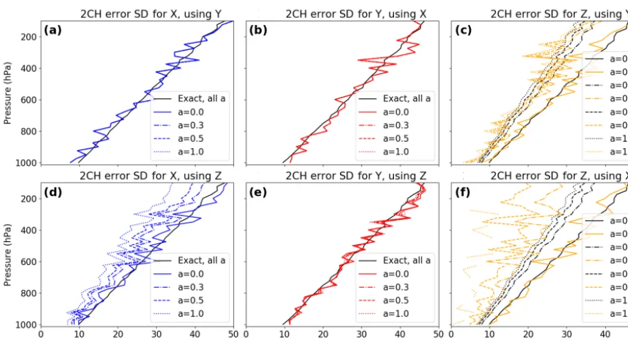
Figure 7 shows the exact and estimated error SD ofX,Y
andZfor various combinations of the data sets and values of
a. The estimated error SD forX,Y andZ vary around the exact solutions (black lines) for all values ofa if data sets with uncorrelated errors are combined: (a) SDerr(X) com-puted withY, (b) SDerr(Y )computed withX, (c) SDerr(Z) computed withY and (e) SDerr(Y )usingZ. Note that in (c) the exact SDerr(Z)decreases withaincreasing from 0 to 1, as described previously. Figure 7d and f show how correlated
errors between the data sets affect the estimated error vari-ances. Both the estimated SDerr(X) and SDerr(Z) become too small when the data setsXandZare combined and the value ofais increased. The exact solutions for all values of
ain (Fig. 7f) are in black.
4.4 Comparison of 3CH and 2CH methods using the error model
4.4.1 Effect of random errors
Figure 8 compares the normalized error estimates from the 3CH and 2CH methods fora=0.5. In Fig. 8a (3CH) the solid lines denote exact error SD ofX,Y andZ. The exact error SD are the same forX and Y and are smaller forZ
as discussed earlier. The estimated error SD (dashed lines) are less than the exact values forX andZ and greater than the exact values forY, also as discussed earlier. In Fig. 8b (2CH), solid lines denote a combination of data sets with un-correlated errors (where error terms are neglected, but are non-zero due to a finite sample size), while dashed lines in-dicate combinations of data sets with correlated errors and neglected error terms. We see that for the 3CH method and 2CH method all estimates are similar, with the exception of SDerr(Y ), which is affected in the 3CH method by correlation ofXerrandZerr. However, the profiles of the 2CH estimates show considerably more noise than those of the 3CH esti-mates, which is a consequence of the larger magnitude of the neglected error terms in the 2CH method (see Sects. 2.3 and 4 above).
Figure 5.Terms involving products of true and (Xerr+Zerr), (Xerr+Yerr) and (Yerr+Zerr) for(a)a=0 and(b)a=0.5. Note that the magnitudes of true and (Xerr+Yerr) and true and (Yerr+Zerr) do not depend on the correlation betweenXerrandZerr. All error terms are normalized.
Figure 6.Mean of products of true andXerr,YerrandZerrfor(a)a=0 and(b)a=0.5. All error terms are normalized.
Figure 9 shows the same estimates as those in Fig. 8, ex-cept for the much smaller sample size of 146. For the smaller sample size, the noise increases for both methods. However, the effect on the 3CH method is less than on the 2CH method, and the differences in the estimates are still clearly visible in the 3CH method. For some of our comparison data sets using real data (Anthes and Rieckh, 2018), the sample sizenis less than 100 in the lower and upper troposphere; hence the noise due to small sampling size is likely to be significant in the estimates for these regions.
4.4.2 Effect of bias errors
To investigate the effect of both random and systematic er-rors, we add a known biasto data setZ.
For the 3CH method, Eq. (3a) becomes VARerr(X)est=
1
2[MS(X−Y )+MS(X−(Z+)) −MS(Y−(Z+))], (15) which may be expanded to
VARerr(X)est= 1
2[MS(X−Y )+MS(X−Z)
−MS(Y−Z)]+M[(Yerr−Xerr)], (16) which is equal to Eq. (3a) plus the bias term. For random errors and a large sample size the means ofXerrandYerrwill be very small and the difference of the mean errors will also be small. Thus the bias term will tend toward zero as the sample size increases and the effect of a bias error inZ is minimal in the 3CH method.
This is not the case in the 2CH method, as shown below. Equation (6a) becomes
VARerr(X)est=MS(X)− 1
4[MS(X+(Z+))
−MS(X−(Z+))] (17) which can be expanded to
VARerr(X)est=MS(X)− 1
4[MS(X+Z)
−MS(X−Z)]−M(X) (18) which is equal to Eq. (6a) plus a bias term.
Figure 7.Two 2CH results each for the normalized error SD forX(a, d),Y (b, e)andZ(c, f), depending on the second data set. Profiles corresponding to several values of correlation parameteraare included. The solid black profile is the exact error SD profile forXandYfor all values ofa, and forZwhena=0.
Figure 8.Estimated and exact normalized error standard deviations for 3CH method(a)and 2CH method(b)for a correlation ofZandX errors of 0.45 (a=0.5).(a)Exact SD errors forX,Y andZare given by blue, red and orange solid lines, respectively. Estimated error SD error is given by dashed lines of same color.(b)Exact error SD ofZis given by solid black line. Estimated error SD ofXusingZandY is given by blue lines, estimated error SD ofY usingXandZis given by red lines, and estimated error SD ofZusingXandY is given by orange lines. For all colored lines, error terms are neglected. Solid lines indicate estimates from combinations of data sets with uncorrelated errors, dashed lines indicate estimates from combinations of data sets with correlated errors and hence larger error terms.
VARerr(X)significantly. The bias term of the 2CH method will stabilize with higher sample sizes around the product of the bias () and theM(X)and will significantly influence the estimated error variance. A positive bias in the data setZwill cause a negative error in VARerr(X), and a negative bias in the data setZwill cause a positive error in VARerr(X).
For the simulated data set, Eq. (10) becomes
Zerr=
a·Xerr+Qerr
1+a +, (19)
whileXerrandYerrstay the same.
Figure 10 shows the effect of adding a constant bias of 10 % toZfor the 3CH and 2CH methods for no correlation of random errors (a=0). For the 3CH method (Fig. 10a), results still look reasonable, and the estimated and exact so-lutions overlap well. For the 2CH method (Fig. 10b), a bias of 10 % strongly impacts the estimated error variances. For
Figure 9.Same as Fig. 8 except for a smaller sample size of 146. All profiles become much noisier, with the 2CH method showing signifi-cantly more noise than the 3CH method.
Figure 10.Effect of adding a constant bias of 10 % toZfor the 3CH(a)and 2CH(b)methods, for no correlation betweenXandZerrors (i.e.,a=0). The 3CH method yields reasonable estimates for all variables, while the estimated error variances from the 2CH method are erroneously large forZ(orange) and erroneously lowXandY (blue and red).
normalized by the sample mean q,M(X)in Eq. (18) is ap-proximately 100 %, so the term M(X) is approximately 100 %2. For=10 %, this term is 1000 %2, which is the offset we see forX,Y andZin Fig. 10b.
4.4.3 General expression for effect of biases in all three data sets
More generally, we can derive expressions for the effect of biases of all three data sets with respect to true as follows (Sergey Sokolovskiy, personal communication, 2018): let
X=true+Xerr+X, (20)
Y =true+Yerr+Y, (21)
Z=true+Zerr+Z, (22)
where X, Y and Z are biases of X, Y and Z, respec-tively. Substituting these expressions into Eq. (3a) for the 3CH method and Eq. (6a) for the 2CH method, we find that the difference1between the error estimates forXwith
bi-ases and those without bibi-ases is
12CH=M(true)(X−Y)+X2 −XY, (23)
13CH=X2−XY−XZ+YZ. (24)
The first term of Eq. (23) is a first-order term while all the other terms are second order; thus in general biases will have a larger effect in the 2CH method compared to the 3CH method. We note that these expressions are valid only for an infinite data set.
5 Estimates of error variances using 3CH and 2CH methods and real observations
sets. Data pairs at each level are only used when data are available for all four data sets. All data sets are interpolated to a common 25 hPa grid. Figure 11a shows the number of co-located profiles per pressure level. Figure 11b shows the normalized RS specific humidity values for these profiles.
The two model and the RO data sets are representative of similar horizontal scales (∼100 km), while the RS data are in situ point measurements and therefore represent a much smaller horizontal scale. However, many studies (e.g., Ho et al., 2010a, b; Kuo et al., 2004; Chen et al., 2011) have used RS data as correlative data for verifying models, RO and other data sets without applying corrections for repre-sentativeness errors. These results indicate that the different representative scales are not a significant source of error in the comparisons (unlike spatial and temporal sampling er-rors resulting from the time and spatial differences between the data sets, which we correct for). However, any representa-tiveness errors are included in the error estimates using either the 2CH or 3CH method.
All four data sets have some degree of unknown bias for certain locations, altitudes or atmospheric conditions; none of them represent the ultimate “truth” and there is no standard atmospheric data set for calibration. However, they have all been compared to other models or observations to one degree or another. We investigated the effect of biases in a related pa-per by Anthes and Rieckh (2018) by calibrating the data sets to the ERA data set using the scaling coefficients as given by Stoffelen (1998) and Vogelzang et al. (2011). The results us-ing the calibrated data sets were very similar to those usus-ing the uncalibrated data sets, confirming that the 3CH method is insensitive to small biases.
We use our results from the 3CH method for real data (An-thes and Rieckh, 2018) to evaluate the results of the 2CH method. Figure 12a shows the 3CH estimated error variances for specific humidity for ERA, RS and RO using three in-dependent equations (Anthes and Rieckh, 2018). The mean value of the estimates is given by the solid line and the SD of the estimates about the mean by the shading. The 3CH estimates are considered reasonably accurate for the reasons given in Anthes and Rieckh (2018), namely that the magni-tude and shape of the estimates for refractivity agree with other independent refractivity error estimates (so we assume that the method works just as well for humidity as for refrac-tivity), and that the results are consistent for the four different RS stations studied.
tained for 2CH estimates of refractivity (not shown). Thus we find that the 2CH method produces estimates of the error variances for specific humidity that are quite dif-ferent from those of the 3CH method. We suspected that the cause for the different behavior using real data might lie in the different treatment of bias errors in the 2CH and 3CH method. To investigate this hypothesis, we considered the ef-fect of an empirically based bias in the simulated data. 5.1 Simulating the observed real data bias in the 2CH
method
As shown in Sect. 4.4.2, even small bias errors in one of the data sets can cause large errors in the 2CH method. To see whether a bias in our real data could explain the very different estimates of the error variances shown in Fig. 12b– d for the 2CH method, we set up empirically based bias profiles in the simulated data. These match approximately the observed differences of RS and RO from ERA as found by Rieckh et al. (2018) in the real data sets (Supplement, Fig. S5 panel 4 for RS; Fig. S6 panel 1 for RO). For the tests we consider ERA the truth. We computed the specific humidity annual mean biases of RO and RS for each level as 100[mean(RO)−mean(ERA)]/mean(ERA) and 100[mean(RS)−mean(ERA)]/mean(ERA), respectively. We used these results to create a simple additive bias for both
Y andZ. The biases are depicted in Fig. 13 (dashed lines), along with the real RS and RO annual mean biases (solid lines). More specifically, the bias used forY (simulating the RO bias) varies linearly between pressure levels as
– −5 to 2 % from 1000 to 800 hPa – 2 to−4 % from 800 to 650 hPa – −4 to 5 % from 650 to 500 hPa – 5 to−11 % from 500 to 300 hPa.
The bias used forZ(simulating the RS bias) varies linearly between pressure levels as
Figure 11. (a)Number of co-located measurements (data pairs) per pressure level for RO, RS and ERA.(b) Normalizedq values for radiosondes (RS) at Mina, 2007. The normalized qvalues are computed as 100·q/q, whereqis the annual mean value ofqfor 2007. Profiles cut off at 250 hPa because RS data are not reported at higher levels. At the bottom, co-located profiles thin out since RO penetration depth varies and only very few profiles are available at the lowest levels.
Figure 12.Estimated error variances for specific humidity:(a)results from the 3CH method for ERA (purple), RO (blue) and RS (orange). Other three panels: 2CH method estimates for ERA(b), RO(c)and RS(d).
The respective bias is added to bothY andZwhen the data are created from the true profiles:
X=true+Xerr; corresponds to ERA
Y =true+Yerr; corresponds to RO
Z=true+Zerr; corresponds to RS.
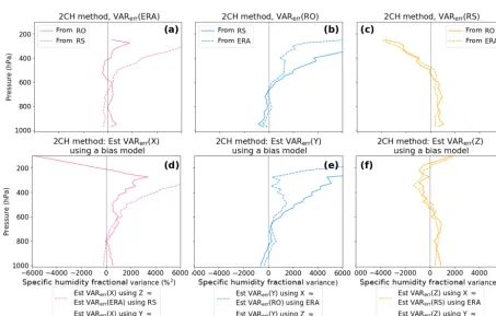
We use these specified biased data sets to compute error variances via the 2CH method. Results are shown in Fig. 14, with the results of the real data in the top row (a–c) and the results of the simulated bias data in the bottom row (d–f).
Figure 13. (a)Annual mean normalized profiles of RS–ERA, RO–ERA and RS–RO.(b)Same for RS–ERA and RO–ERA only (solid lines), and their respective empirical bias profiles (dashed lines) based on the mean profiles.
Figure 14.2CH method error variances for ERA, RO and RS(a–c)and for simulated data using the specified empirical bias profiles(d–f). Correlation betweenXandZerrors is zero for this experiment.
responsible for the results using real data and how they vary from the 3CH method results.
6 Summary and conclusions
In this study we compared two methods for estimating the error variances of multiple data sets, the three-cornered hat (3CH) and two-cornered hat (2CH) methods. Using a simu-lated data set in which we could vary the degree of
esti-mates by repeating the calculations using a subset of 146 of the total 1460 profiles. We found that the 3CH method was less sensitive to the neglected error terms for various random error correlations than the 2CH method. We also showed that the effect of bias errors on one of the data sets had a relatively small effect on the 3CH method, but produced much larger errors in the 2CH method.
We also compared the 3CH and 2CH methods using real RS, radio occultation (RO) and ERA data. We find that the 3CH method produces more consistent and accurate results than the 2CH method when using real data. The 2CH method produced very different estimates of the error variance of ERA depending on which observational data set (e.g., RS or RO) was used in the comparison. Using an empirical bias model based on observed RS and RO difference from ERA during 2007, we showed that these differences in error vari-ance estimates were likely caused by different biases in the RS and RO data. The effect of bias errors is shown to give unrealistic results using the 2CH method.
Code availability. Code will be made available by the author upon request.
Equation (A3) is summed over all the data pairs to get 1
n X
(X+Z)2=41
n X
true2 +1
n X h
(Xerr+Zerr)2+4true(Xerr+Zerr) i
. (A4)
Defining the following expressions:
M(X)= 1
n X
X
M(X, Y )=M(X·Y )=1
n X
X×Y.
Eq. (A4) becomes
MS(X+Z)=4MS(true)+VARerr(X)+VARerr(Z)
+2COVerr(X, Z)+4M(true, Xerr+Zerr).
(A5)
We then subtractZ fromX and square the difference to get
MS(X−Z)=VARerr(X)+VARerr(Z)
−2COVerr(X, Z). (A6)
and substituting forMS(true) from Eq. (A7) gives VARerr(X)=MS(X)−
1
4[MS(X+Z)−MS(X−Z)] −2M(true, Xerr)+COVerr(X, Z)
+M(true, Xerr+Zerr). (A9) Similarly, we obtain
VARerr(Z)=MS(Z)−1
4[MS(X+Z)−MS(X−Z)] −2M(true, Zerr)+COVerr(X, Z)
Author contributions. Both authors contributed equally to the ideas and conceptual development. The first author computed the results.
Competing interests. The authors declare that they have no conflict of interest.
Acknowledgements. The authors were supported by NSF-NASA grant AGS-1522830. We thank Shay Gilpin for Fig. 4 and the two reviewers for their comments on the original draft. John Eyre (Met Office) provided useful insights and comments on drafts of the manuscript. We thank Eric DeWeaver (NSF) and Jack Kaye (NASA) for their long-term support of COSMIC.
Edited by: Ad Stoffelen
Reviewed by: two anonymous referees
References
Anthes, R. and Rieckh, T.: Estimating observation and model er-ror variances using multiple data sets, Atmos. Meas. Tech., 11, 4239–4260, https://doi.org/10.5194/amt-11-4239-2018, 2018. Braun, J., Rocken, C., and Ware, R.: Validation of line-of-sight
water vapor measurements with GPS, Radio Sci., 36, 459–472, 2001.
Chen, S.-Y., Huang, C.-Y., Kuo, Y.-H., and Sokolovskiy, S.: Ob-servational Error Estimation of FORMOSAT-3/COSMIC GPS Radio Occultation Data, Mon. Weather Rev., 139, 853–865, https://doi.org/10.1175/2010MWR3260.1, 2011.
Collard, A. D. and Healy, S. B.: The combined impact of future space-based atmospheric sounding instruments on numerical weather-prediction analysis fields: A simu-lation study, Q. J. Roy. Meteor. Soc., 129, 2741–2760, https://doi.org/10.1256/qj.02.124, 2003.
Dee, D. P., Uppala, S. M., Simmons, A. J., Berrisford, P., Poli, P., Kobayashi, S., Andrae, U., Balmaseda, M. A., Balsamo, G., Bauer, P., Bechtold, P., Beljaars, A. C. M., van de Berg, L., Bid-lot, J., Bormann, N., Delsol, C., Dragani, R., Fuentes, M., Geer, A. J., Haimberger, L., Healy, S. B., Hersbach, H., Hólm, E. V., Isaksen, L., Kållberg, P., Köhler, M., Matricardi, M., McNally, A. P., Monge-Sanz, B. M., Morcrette, J.-J., Park, B.-K., Peubey, C., de Rosnay, P., Tavolato, C., Thépaut, J.-N., and Vitart, F.: The ERA-Interim reanalysis: configuration and performance of the data assimilation system, Q. J. Roy. Meteor. Soc., 137, 553–597, https://doi.org/10.1002/qj.828, 2011.
Desroziers, G. and Ivanov, S.: Diagnosing and adaptive tuning of observation-error parameters in a variational assimilation, Q. J. Roy. Meteor. Soc., 127, 1433–1452, https://doi.org/10.1002/qj.49712757417, 2001.
Ekstrom, C. R. and Koppang, P. A.: Error Bars for Three-Cornered Hats, IEEE Trans. Ultrason. Ferroelect. Freq. Contr., 53, 876– 879, https://doi.org/10.1109/TUFFC.2006.1632679, 2006. Gray, J. E. and Allan, D. W.: A method for estimating the frequency
stability of an individual oscillator, Atlantic City, New Jersey, 29–31 May, 1974.
Griggs, E., Kursinski, E., and Akos, D.: An investigation of GNSS atomic clock behaviour at short time intervals, GPS Solut., 18, 443–452, https://doi.org/10.1007/s10291-013-0343-7, 2014. Griggs, E., Kursinski, E., and Akos, D.: Short-term
GNSS satellite clock stability, Radio Sci., 50, 813–826, https://doi.org/10.1002/2015RS005667, 2015.
Gruber, A., Su, C.-H., Zwieback, S., Crow, W., Dorigo, W., and Wagner, W.: Recent advances in (soil moisture) triple colloca-tion analysis, Int. J. Appl. Earth Obs. Geoinf., 45, 200–211, https://doi.org/10.1016/j.jag.2015.09.002, 2016.
Ho, S.-P., Kuo, Y.-H., Schreiner, W., and Zhou, X.: Using SI-traceable Global Positioning System radio occultation measure-ments for climate monitoring, B. Am. Meteorol. Soc., 91, S36– S37, 2010a.
Ho, S.-P., Zhou, X., Kuo, Y.-H., Hunt, D., and Wang, J.-H.: Global evaluation of radiosonde water vapor systematic biases using GPS radio occultation from COSMIC and ECMWF analysis, Re-mote Sens., 2, 1320–1330, https://doi.org/10.3390/RS2051320, 2010b.
Kuo, Y.-H., Wee, T.-K., Sokolovskiy, S., Rocken, C., Schreiner, W., Hunt, D., and Anthes, R. A.: Inversion and error estimation of GPS radio occultation data, J. Meteor. Soc. JPN, 82, 507–531, 2004.
Kursinski, E. R., Hajj, G. A., Schofield, J. T., Linfield, R. P., and Hardy, K. R.: Observing Earth’s atmosphere with radio occultation measurements using the Global Po-sitioning System, J. Geophys. Res., 102, 23429–23465, https://doi.org/10.1029/97JD01569, 1997.
Luna, D., Pérez, D., Cifuentes, A., and Gómez, D.: Three-Cornered Hat Method via GPS Common-View Compar-isons, IEEE Trans. Instrument. Measure., 66, 2143–2147, https://doi.org/10.1109/TIM.2017.2684918, 2017.
O’Carroll, A. G., Eyre, J. R., and Saunders, R. S.: Three-way er-ror analysis between AATSR, AMSR-E, and in situ sea surface temperature observations, J. Atmos. Ocean. Technol., 25, 1197– 1207, https://doi.org/10.1175/2007JTECHO542.1, 2008. Rieckh, T., Anthes, R., Randel, W., Ho, S.-P., and Foelsche, U.:
Evaluating tropospheric humidity from GPS radio occultation, radiosonde, and AIRS from high-resolution time series, At-mos. Meas. Tech., 11, 3091–3109, https://doi.org/10.5194/amt-11-3091-2018, 2018.
Riley, W. J.: Application of the 3-cornered hat method to the anal-ysis of frequency stability, available at: http://www.wriley.com/ 3-CornHat.htm (1 July 2018), 2003.
Roebeling, R. A., Wolters, E. L. A., Meirink, J. F., and Leijnse, H.: Triple collocation of summer precipitation re-trievals from SEVIRI over Europe with gridded rain gauge and weather radar data, J. Hydrometeorol., 13, 1552–1566, https://doi.org/10.1175/JHM-D-11-089.1, 2012.
Stoffelen, A.: Toward the true near-surface wind speed: Error mod-eling and calibration using triple collocation, J. Geophys. Res., 103, 7755–7766, https://doi.org/10.1029/97JC03180, 1998. Su, C.-H., Ryu, D., Crow, W. T., and Western, A. W.:
Beyond triple collocation: Applications to soil mois-ture monitoring, J. Geophys. Res., 119, 6419–6439, https://doi.org/10.1002/2013JD021043, 2014.