https://doi.org/10.5194/esd-9-1045-2018 © Author(s) 2018. This work is distributed under the Creative Commons Attribution 4.0 License.
Improving the representation of
anthropogenic
CO
2
emissions in climate
models: impact of a new parameterization
for the Community Earth System Model (CESM)
Andrés Navarro, Raúl Moreno, and Francisco J. Tapiador
Institute of Environmental Sciences (ICAM), University of Castilla–La Mancha, 45004 Toledo, Spain Correspondence:Andrés Navarro ([email protected])
Received: 27 February 2018 – Discussion started: 19 March 2018 Revised: 11 July 2018 – Accepted: 23 July 2018 – Published: 21 August 2018
Abstract. ESMs (Earth system models) are important tools that help scientists understand the complexities of the Earth’s climate. Advances in computing power have permitted the development of increasingly complex ESMs and the introduction of better, more accurate parameterizations of processes that are too complex to be described in detail. One of the least well-controlled parameterizations involves human activities and their di-rect impact at local and regional scales. In order to improve the didi-rect representation of human activities and climate, we have developed a simple, scalable approach that we have named the POPEM module (POpulation Parameterization for Earth Models). This module computes monthly fossil fuel emissions at grid-point scale using the modeled population projections. This paper shows how integrating POPEM parameterization into the CESM (Community Earth System Model) enhances the realism of global climate modeling, improving this be-yond simpler approaches. The results show that it is indeed advantageous to model CO2emissions and pollutants directly at model grid points rather than using the same mean value globally. A major bonus of this approach is the increased capacity to understand the potential effects of localized pollutant emissions on long-term global climate statistics, thus assisting adaptation and mitigation policies.
1 Introduction
The Earth system is a complex interplay of physical, chemi-cal, and biological processes that interact in nonlinear ways (Ladyman et al., 2013; Lorenz, 1963; Rind, 1999; Williams, 2005). Much effort has been devoted to understanding these complex interactions, and several improvements have been made since the end of the last century.
One of the most important advances in this field has been the use of coupled numerical climate models, dubbed Earth system models or ESMs (Edwards, 2011; Flato, 2011; Schellnhuber, 1999). These models aim to simulate the com-plex interactions of the atmosphere, ocean, land surface, and cryosphere, together with the carbon and nitrogen cycles (Giorgetta et al., 2013; Hurrell et al., 2013; Martin et al., 2011; Schmidt et al., 2014).
However powerful, climate models are far from being per-fect (Hargreaves, 2010; Hargreaves and Annan, 2014). Un-resolved processes (Williams, 2005), limited computational resources (Shukla et al., 2010; Washington et al., 2009), and model uncertainties (Baumberger et al., 2017; Lahsen, 2005; Steven and Bony, 2013) are ongoing issues that still require attention and further improvement.
et al., 2011). However, most global models use basic so-cioeconomic assumptions about the behavior of societies and are only unidirectionally linked to the biogeophysical part of the Earth system (Müller-Hansen et al., 2017; Smith et al., 2014). The standard way of introducing anthropogenic cli-mate change into ESMs is through representative concentra-tion pathways (RCPs). These are consistent sets of projec-tions involving only radiative forcing components (van Vu-uren et al., 2011), but which represent a step forward from the scenario approach of the last decade (Moss et al., 2010; van Vuuren et al., 2014; van Vuuren and Carter, 2014). How-ever, RCPs are not fully integrated socioeconomic parame-terizations but rather estimates for describing plausible tra-jectories of human climate change drivers (Moss et al., 2010; van Vuuren et al., 2012). They provide simplified accounts of human activities and processes from one-way coupled in-tegrated assessment models (IAMs; Müller-Hansen et al., 2017).
The use of RCPs is advantageous because they provide a set of pathways that serve to initialize climate models. However, two major problems remain within this approach. Firstly, human activities are not intrinsically embedded into the ESM, impeding sensitivity studies. Secondly, because of the weak coupling of IAMs, they cannot capture the sometimes counterintuitive bidirectional feedback and non-linearity between the socioeconomic and natural subsystems (Motesharrei et al., 2016; Ruth et al., 2011). Good examples that illustrate the importance of including such bidirectional feedbacks feature in the HANDY model (Motesharrei et al., 2014) which has been used to analyze the key mechanisms behind societal collapses.
The RCP approach has been used in climate models be-cause of its low computational cost. However, advances in computational resources now allow to parameterize human– Earth processes in a more detailed way, including the in-clusion of population dynamics into the modeling, as in the POPEM (POpulation Parameterization for Earth Models) module (Navarro et al., 2017).
One important, but sometimes overlooked, process is the direct regional effect of anthropogenic greenhouse gas (GHG) emissions. Although some GHGs quickly mix in the atmosphere (IPCC, 2014a), their mixing times and life-times vary (Archer et al., 2009; Prather, 2007), and local-ized emissions may produce a transient response in the atmo-sphere. Given the highly nonlinear character of the processes involved, it is not unreasonable to assume that accounting for geographical variability is significant, and the spatial and time distribution of these emissions may affect global cli-mate (Alter et al., 2017; Grandey et al., 2016; Guo et al., 2013). This hypothesis has seldom been investigated, as most current models treat certain GHG emissions as a homoge-neously distributed forcing. Thus, for instance, the most typ-ical CESM (Community Earth System Model) simulations prescribe a CO2 concentration on the assumption that it is well mixed in the atmosphere (Neale et al., 2012).
This paper describes the results of a 50-year simulation with a simple parameterization of fossil fuel CO2emissions at model grid-point scale, integrating the POPEM module into the CESM. The aim of this paper is to show that this grid-point scale modeling of anthropogenic CO2emissions (and other pollutants) represents an improvement over sim-pler approaches, and leads to better representation of the ge-ographical variability of precipitation.
The purpose of the new modeling is not only to improve precipitation and temperature estimates but also to help un-derstand the carbon cycle feedback, and evaluate the climate sensitivity of the Earth under alternative GHG emission sce-narios. While our focus here is anthropogenic CO2 emis-sions, the POPEM parameterization can accommodate other GHGs and human-dependent processes in order to advance CESMs towards a comprehensive fully coupled modeling of anthropogenic dynamics in the global climate.
The paper is organized as follows: in Sect. 2, we present the validation of the POPEM stand-alone mode and set the framework for evaluating the impact of POPEM parameter-ization – its incorporation into the CESM and the testing framework; in Sect. 3, we compare the outputs of CONTROL and POPEM runs and see how they compare with obser-vations. In Sect. 4, we highlight the importance of the dy-namical modeling of anthropogenic emissions at grid-point scale to better represent the socioeconomic parameters in the CESM model and improve precipitation estimates.
2 Material and methods
2.1 The CESM model
The Community Earth System Model (CESM) is a state-of-the-art ESM and probably the most widely used climate model. It was developed and is maintained by the National Center for Atmospheric Research (NCAR), with contribu-tions from external researchers funded by the US Department of Energy, the National Aeronautics and Space Administra-tion (NASA), and the NaAdministra-tional Science FoundaAdministra-tion (Hurrell et al., 2013). CESM is an ESM comprising a system of multi-geophysical components, which periodically exchange two-dimensional boundary data in the coupler (Craig et al., 2012). It consists of five component models and one central cou-pler component: the atmosphere model CAM (Community Atmosphere Model; Tilmes et al., 2015); the ocean model POP (Parallel Ocean Program; Kerbyson and Jones, 2005); the land model CLM (Community Land Model; Lawrence et al., 2011); the sea ice model CICE (Community Ice Code; Hunke and Lipscomb, 2008); and the ice sheet model CISM (Community Ice Sheet Model; Lipscomb et al., 2013).
evolved into a complex Earth system model now used in different fields. This includes research into atmospheric (Bacmeister et al., 2014; Liu et al., 2012; Yuan et al., 2013), biogeochemical (Lehner et al., 2015; Nevison et al., 2016; Val Martin et al., 2014), and human-induced processes (Huang and Ullrich, 2016; Levis et al., 2012; Oleson et al., 2011), as well as others. The core code of CESM has also been utilized by various research centers for developing their own models (norESM; Bentsen et al., 2013; CMCC–CESM– NEMO; Fogli and Iovino, 2014; MIT IGSM-CAM; Monier et al., 2013). CESM has been used in many hundreds of peer-reviewed studies to better understand climate variability and climate change (Hurrell et al., 2013; Kay et al., 2015; Sander-son et al., 2017). Simulations performed with CESM have made a significant contribution to international assessments of climate, including those of the Intergovernmental Panel on Climate Change (IPCC) and the CMIP5/6 project (Cou-pled Model Intercomparison Project Phase 5/6) (Eyring et al., 2016; IPCC, 2014b; Taylor et al., 2012).
A major advantage of CESM over other ESMs is its availability. Some climate models are developed by scien-tific groups and access to the source code is limited. The CESM source code is free and available to download from the NCAR website. This approach helps improve the model by setting up a framework for collaborative research and makes the model fully auditable. CESM is a good example of a “full confidence level” model, after Tapiador et al. (2017), where many “avatars” of the code are routinely run in sev-eral independent research centers, and there is an entire com-munity improving the model and reporting on issues and re-sults. However, the model is not immune to bias. One im-portant shortcoming is the poor representation of precipita-tion in terms of spatial structure, intensity, duraprecipita-tion, and fre-quency (Dai, 2006; Tapiador et al., 2018; Trenberth et al., 2015, 2017). Another major bias is the anomalous warm sur-face temperature in coastal upwelling regions (Davey et al., 2002; Justin Small et al., 2015; Richter, 2015).
2.2 POPEM specifics and stand-alone validation 2.2.1 POPEM parameterization model overview
The POPEM module is a demographic projection model coded in FORTRAN that is intended to estimate monthly fos-sil fuel CO2emissions at model grid-point scale using pop-ulation as the input. Due to a lack of actual GHG measure-ments at appropriate spatial and temporal scales, it is neces-sary to use a proxy. For this, POPEM employs population, the evolution of which is modeled using external parameters that feed the module. The idea of using population as proxy is not new, and population density has previously been used to downscale national CO2 emissions (Andres et al., 1996, 2016). However, these inventories were not dynamical but instead tied to historical data so it is not possible to use them either to estimate future changes in emissions or coupled
with other components of the model. This change represents an important advance in the way emissions are computed. Thus, POPEM uses a bottom-up approach, where emissions are calculated at cell level on the basis of population pro-jections, while global inventories use a top-down approach, which is less flexible when coupled with other components of the ESM.
The demographic/emissions module presented here is an updated version of the demographic module explained in Navarro et al. (2017). The differences between the versions are minimal. They involve better approximation of emissions in highly polluting regions with poor population data, such as China; a better estimate for coastal zones and country limits; and a change in the model time step for more efficient cou-pling with CESM. The inclusion of these changes results in more accurate emission estimates when compared with in-ventories than the previous version did. However, the model is not immune to bias. The most important limit is the degra-dation of the model outputs when there is increased spatial resolution – resolution of 0.25◦and higher.
Detailed information on POPEM and its validation in the demographic realm can be found in Navarro et al. (2017). In short, from an initial condition, the routine computes the population for each model grid point in a 2-D matrix and then calculates fossil fuel CO2 emissions using per capita emission rates by nations. The process is repeated for each time step (e.g., annually) throughout the simulation period.
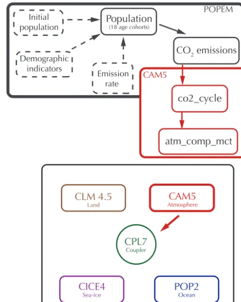
As seen in Fig. 1, POPEM stores gridded emission data in a 3-D array (time, latitude, and longitude) to be used by the modified version of theco2_cyclemodule. This module reads emission data and passes this to theatm_comp_mct, which calculates the total amount of CO2emissions from dif-ferent sources (land, ocean, and fossil fuel).
2.2.2 POPEM trend verification
Prior to coupling POPEM with CESM, we performed sev-eral tests to evaluate its ability to reproduce historical popu-lation trends and CO2emissions. To do this, we ran the mod-ule in stand-alone mode. In a first test, we ran a short sim-ulation (1950–2013) and compared the emission data with a standard emissions inventory (CDIAC). In a second test, POPEM was run for 70 years (1950–2020) and population estimates were validated against the UN (United Nations) population statistics database for those years when data were available.
popu-CLM 4.5
Land
POP2
Ocean CICE4
Sea-ice
CAM5
Atmosphere
CPL7
Coupler
Population (18 age cohorts)
atm_comp_mct
Initial population
Emission rate Demographic
indicators
CO2 emissions
co2_cycle
CAM5
POPEM
RTM
River transport GLIMMER-CISMLand ice CESM 1.2.2
co2flux_fuel (t,lat,lon)
nqx(t,age,ctry) co_emrate(t,ctry) nfrx(t,age,ctry)
pop_month(t,age,lat,lon)
data_flux_fuel(t,lat,lon)
init_pop(t)
time step=30 min
Time step= monthly
Figure 1. Conceptual scheme of the POPEM module coupled
with the CAM5 atmosphere module. POPEM requires three in-put data sets to comin-pute emissions (black dashed rectangles): ini-tial population distribution; demographic parameters (age structure, death, and birth rates); and per capita emission rates by country. POPEM provides a 3-D array (time, latitude, longitude) with emis-sions that are read by theco2_cyclemodule and passed to the
atm_comp_mctmodule which computes the total amount of CO2
in the atmosphere.
lation in those regions with a more elderly age structure, i.e., Europe and North America, and underestimates areas with younger populations, i.e., Latin America and Asia.
These disparities in population counts have a diverse ef-fect on the outputs in terms of GHG emissions. Thus, for example, the bias in Europe seems to be more important than the bias in Latin America and Oceania. Two principal reasons could explain this: population size, as Europe has a larger population than Oceania, so there is greater bias in the CO2emissions estimation; and the per capita emissions rate, as Latin American countries have lower per capita emission rates than European nations.
It is worth noting here that the POPEM outputs in Fig. 2 are clearly nonlinear and thus not trivially derived from sim-ply extrapolating population. The North American estimate of CO2 emissions (second row from the bottom) clearly shows the added value introduced by the model.
1950
7000 2100
Oceania
1990
1.4
1.0
0.6
0.2
POPEM
8.0
6.0
4.0
2.0
5.0 4.0
2.0 1.0 3.0
0.76
0.68
0.60
0.52 0.7
0.5
0.4
0.1
0.30 0.25 0.20 0.40 0.35
0.02 0.01 0.04
0.03
1950 1970 2010
Year
POPEM
N. America
L. America
Europe
Asia
Africa
W
orld
Year
30 000
20 000
10 000 40 000
15 000 9000
3000 21 000
6000
4000 8000
2000
1500
900
300
5000
3000
300
100
1990 1970 2010
500 900
300 1500
Oceania
N. America
L. America
Europe
Asia
Africa
W
orld
(b) CO emissions
2(a) Population
UN CDIAC
Figure 2. Comparison of the population estimates for the
years 1950–2020 (a)and the historical CO2 emission estimates
for the years 1950–2012(b). The first row compares global data, the second to seventh rows compare regional data (Africa, Europe, Latin America, North America, and Oceania). In(a), the red line shows the estimates given using POPEM and blue indicates UN es-timates. Values are given in billions of people. In(b), the red line shows the estimates given using POPEM and the black indicates CDIAC estimates. Units are given in million metric tons.
1950
1980
2000
1
4.5
8.5
11.5 15.5
19.5
Million metric tons of CO2
180 120° W60°W 0 60°E 120°E 180
30° N
30° S
90° S
90° N
0
30° N
30° S
90° S
90° N
0
30° N
30° S
90° S
90° N
0
Evolution of the CO
2emissions in the POPEM model
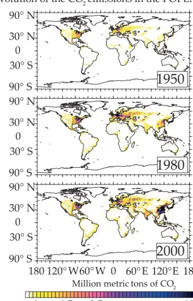
Figure 3. POPEM CO2 emission estimates for 1950, 1980,
and 2000. POPEM produces a gridded representation of anthro-pogenic CO2 emissions using population dynamics and country
per capita emissions derived from the CDIAC database. Values are given in millions of metric tons per year.
maps for the recent past (Andres et al., 1996; Boden et al., 2017; Oda et al., 2018; Rayner et al., 2010), as well as with regional studies on CO2emissions (Gately et al., 2013; Gur-ney et al., 2009).
The regionalized distribution of emissions depicted in Fig. 3 represents a vast improvement over the standard proce-dure of using globally averaged emissions. Even accounting for rapid mixing of GHGs, transient effects are likely to ap-pear given the hemispheric contrast and regional differences in the emissions. The differences in Asia are illustrative of the economic changes in the recent past and the exponential pace of industrialization in that region.
2.3 CESM experimental setup
The CESM used in this work is based on version 1.2.2 (http://www.cesm.ucar.edu/models/, last access: 10 Febru-ary 2018). This set includes active components for the atmo-sphere, land, ocean, and sea ice, all coupled by a flux coupler. The latest atmospheric module CAM5 (Neale et al., 2012) is used to introduce more accurate modeling of atmospheric
physics. Additionally, the carbon cycle module is included in CESM’s atmosphere, land, and ocean components (Lindsay et al., 2014).
We ran an experiment at 1.9◦of spatial resolution for the period 1950–2000. Two simulations were performed to an-alyze the effects of the regionalized emissions (Fig. 3) on the CESM. Our control case used homogeneous CO2 con-centration parameters (standard procedure in ESMs), while the POPEM case used geographically distributed CO2 emis-sion data. In the latter, the POPEM module was coupled with the atmospheric CO2 flux routine to provide monthly grid-ded CO2emissions. The gridded data were used at each time step by the atmospheric routine. Apart from this change, both simulations were identical in order to identify the effects (if any) of the POPEM parameterization.
2.4 Validation data 2.4.1 GPCP data set
Precipitation is one of the key elements for balancing the energy budget, and one of the most challenging aspects of climate modeling. Hence, high-quality estimates of precipi-tation distribution, amount, and intensity are essential (Hou et al., 2014; Kidd et al., 2017; Xie and Arkin, 1997). While there are many sources of precipitation data to be used as a reference (see Tapiador et al., 2012, for a review), only a few qualify as “full confidence level validation data” (Tapiador et al., 2017).
The Global Precipitation Climatology Project (GPCP; Adler et al., 2016) has several products suitable for validating climate models. GPCP-Monthly is one of the most popular precipitation data sets for climate variability studies. It com-bines data from rain gauge stations and satellite observations to estimate monthly rainfall on a 2.5◦global grid from 1979
to the present. The careful combination of satellite-based rainfall estimates results in the most complete analysis of rainfall available to date over the global oceans, and adds necessary spatial detail to rainfall analyses over land. Due to its relevance and global coverage, it has been widely used for validating precipitation in climate models (Li and Xie, 2014; Pincus et al., 2008; Stanfield et al., 2016; Tapiador, 2010).
2.4.2 CRU data set
grid cells covering the global land surface and combined with existing climatology data to obtain absolute monthly values (New et al., 1999, 2000). It is commonly used in the val-idation of climate models because of its confidence levels, together with temporal and spatial coverage, and the fact it compiles station data from multiple variables from numer-ous data sources into a consistent format (Christensen and Boberg, 2012; Hao et al., 2013; Liu et al., 2014; Nasrollahi et al., 2015).
2.4.3 GISTEMP data set
NASA’s GISTEMP (GISS Surface Temperature Analysis) is a global surface temperature change data set (Hansen and Lebedeff, 1987; see Hansen et al., 2010, for an updated ver-sion). It combines land and ocean surface temperatures to create monthly temperature anomalies at 2◦×2◦degrees of spatial resolution. The use of anomalies reduces the estima-tion error in those places with incomplete spatial and tempo-ral coverage (Hansen and Lebedeff, 1987). The anomalies are calculated over a fixed base period (1951–1980) that makes the anomalies consistent over long periods of time.
The first version was originally conceived only for land ar-eas (Hansen and Lebedeff, 1987) but in 1996 marine surface temperatures were added (Hansen et al., 1996). The updated version of GISTEMP includes satellite-observed night lights to identify stations located in extreme darkness and adjust temperature trends of urban stations for non-climatic factors (Hansen et al., 2010). Just like CRUTS, GISTEMP is com-monly used to validate climate models because of its cover-age and confidence levels (Baker and Taylor, 2016; Brown et al., 2015; Neely et al., 2016; Peng-Fei et al., 2015).
3 Results and discussion
3.1 Comparison between the CONTROL and POPEM runs
It is worth stressing that a parameterization which performs well when tested for the variable it models does not neces-sarily translate into an overall improvement of the other vari-ables in the model. An accepted practice in climate model-ing is to tune ESMs by adjustmodel-ing some parameters to achieve a better agreement with observations (Hourdin et al., 2017; Mauritsen et al., 2012). These adjustments to specific tar-gets may, however, decrease the model’s overall performance (Hourdin et al., 2017), and give poor scores for variables other than those tuned. Thus, for example, if a model is bi-ased with respect to aerosol concentrations or humidity, then improved parameterization of cloud formation may worsen the performance of the model with regard to precipitation (Baumberger et al., 2017). This mismatch can be caused by model over-specification, or over-tuning.
The first step in evaluating the new parameterization is to compare the outputs with a control simulation to make sure the new addition does not negatively interact with the dy-namical core or spoil the contributions of the rest of the pa-rameterizations. Figure 4 shows that this is not the case with the POPEM parameterization, which does not negatively af-fect the outputs of precipitation and temperature. Rather, both variables are now closer to the observed data than they were in the control run, especially in terms of reducing the double ITCZ (Intertropical Convergence Zone), which artifi-cially features in global models (Mechoso et al., 1995; for a recent analysis of double ITCZ in CMIP5 models see Oues-lati and Bellon, 2015).
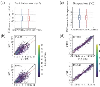
Figure 4a shows that there is just a slight discrepancy in the absolute difference in rainfall between the GPCP and CESM simulations (the first and the third quartiles of the distribution remain between±0.4 mm day−1). Grid-point to grid-point comparison between the model and GPCP indi-cates the ability of CESM to reproduce the spatial distribu-tion of precipitadistribu-tion. In both simuladistribu-tions, the CESM exhibits a good correlation coefficient (0.72R2) compared with the reference data (Fig. 4b). The results are even better for tem-perature (0.88R2; Fig. 4d).
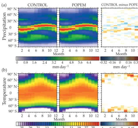
Direct comparison of aggregated data is a standard pro-cedure for gauging model abilities. Figure 5 compares two latitude–time graphs for precipitation (Fig. 5a) and surface temperature (Fig. 5b), both for the CONTROL case and for the new POPEM parameterization.
It is clear from Figs. 5a and 6a that POPEM does alter the spatial pattern of precipitation and exerts a definite effect on the climate pattern, as the module reduces the otherwise exaggerated ITCZ precipitation in the Southern Hemisphere reported by several authors (Hwang and Frierson, 2013; Li and Xie, 2014).
Disparities in temperature between the CONTROL and POPEM runs are apparent at high latitudes. In this case, POPEM produces lower temperatures at both poles, a result which deserves further attention (Figs. 5b and 6b).
There are also important differences in precipitation in the 30◦N–30◦S band. Here POPEM reduces model bias, espe-cially in the Southern Hemisphere and on the Tibetan Plateau (see Sect. 3.2 for more details). On the other hand, POPEM departs from the control simulation in the Asia Pacific region between 10◦N–10◦S. This result reinforces the double ITCZ bias in this area.
al-(a)
(c)
0 4 8 14 12 10
6
2
GPCP
0 4 8 14 12 10
6
2
GPCP
POPEM
CONTROL
0 2 4 6 8 10 12 14 0 2 4 6 8 10 12 14
90 80 70 60 50 40 30 20 10
Counts/bin
R2=0.72
R2=0.72
1 0.5
0 -0.5
-1
Difference in precipitation
Precipitation (mm day-1)
GPCP-POPEM GPCP-CONTROL
-34 -14 4 32 24 14
-4
-24
CR
U
-34 -14 4 32 24 14
-4
-24
CR
U
POPEM
CONTROL
-34 -24 -14 -4 4 14 24 32 -34 -24 -14 -4 4 14 24 32
50
40
30
20
10
Counts/bin
R2=0.88
R2=0.88
5 3 1 -1 -1
-5
D
iffer
ence in temperatur
e
Temperature ( C)
CRU-POPEMCRU-CONTROL
-3
(b)
(d)
Figure 4.Box plots of CESM simulation bias for precipitation(a)and temperature(c).(b)Scatter plots comparing the annual mean
precip-itation (1980–2000) at every grid point for GPCP and CESM simulations (POPEM and CONTROL).(d)Scatter plots comparing the annual mean temperature at every grid point for CRU and CESM simulations (POPEM and CONTROL). Units are in mm day−1(precipitation) and in◦C (temperature).
low for precise emissions modeling in the future. This is an important aspect for regionalized emission scenarios, since even if the new parameterization is not significantly better than the old approach (but no worse), it is desirable as it al-lows for sensitivity analyses, such as evaluating the effects of the US leaving the Paris Agreement.
Potential applications of POPEM include not only sensi-tivity analyses of local CO2 emissions policies but also the added feature of performing tests for “what if” scenarios. One interesting example would be the climate response un-der the hypothesis that China and India – the most populated countries in the world – reach US CO2per capita emission rates. Another “what if” scenario would be the climate re-sponse of an increasingly urbanized world. In both cases, POPEM provides a flexible framework for testing the alter-native hypotheses.
The realism of the ESM will be enhanced with a fully cou-pled system. Such a fully fledged ESM will include bidirec-tional feedback between POPEM and CESM to evaluate the effects of climate change on population dynamics and emis-sions.
3.2 Validation against observational data sets
Once it has been verified that the new parameterization does not worsen the modeling, the next step in evaluating the per-formances is comparing the simulation outputs for both the CONTROL run and the POPEM module using actual obser-vational data. Direct comparisons with historical data can help show whether or not a climate model correctly repre-sents the climate of the past. However, although observa-tional measurements are often considered the ground truth to validate models against, it is important to be aware that measurements have their own uncertainties (Tapiador et al., 2017).
Figure 7 shows a comparison of CESM precipitation sim-ulations for the period 1980–2000 using the GPCP. It is ap-parent that there is an overall consensus, even though there are differences. Despite these known biases, the model agrees with the observations on the major features of global precip-itation.
refer-30° N
30° S
90° S 90° N
0 60° N
60° S
0 0.8 1.6 2.4 3.2 4 4.8 5.6 6.4 -0.32 -0.16 0 0.16 0.32
2 4 6 8 10 12 2 4 6 8 10 12 2 4 6 8 10 12
mm day-1 mm day CONTROL POPEM CONTROL minus POPEM
Month Month
-35 -29 -21 -13 3 11 19 27 35 -1 -0.45 0 0.45 1
2 4 6 8 10 12 2 4 6 8 10 12 2 4 6 8 10 12
º C º C
Month
-5
Month (a)
Precipitation
T
emper
ature
(b)
30° N
30° S
90° S 90° N
0 60° N
60° S
-1
Figure 5.Latitude vs. time plots for precipitation(a)and surface
temperature (b). For absolute difference graphs, blue represents higher values in POPEM and red represents higher values in the CONTROL. Units are in mm day−1for precipitation and in◦C for temperature.
ence data. This observation illustrates the limitations of the modeling and the need of advances in the parameteriza-tions. However, for this area the correlation (R2) between POPEM and GPCP is slightly better than CONTROL and GPCP (0.706R2versus 0.692R2).
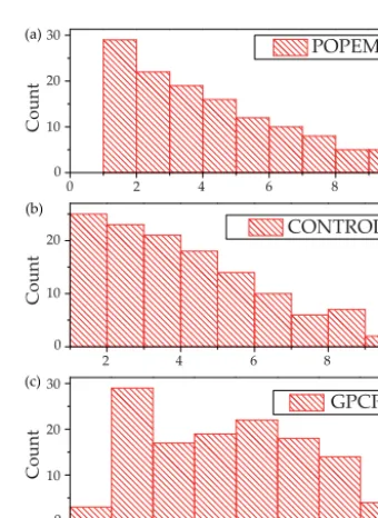
The real added value, however, is not in a better estima-tion of the totals but in the ability of POPEM to better cap-ture the struccap-ture of the precipitation. Figure 8 shows the his-tograms of mean precipitation in the El Niño-4 area using the POPEM parameterization (Fig. 8a), the standard forcing approach (CONTROL, Fig. 8b), and the reference GPCP es-timates (Fig. 8c). While the CONTROL simulation severely overestimates the low end of the distribution, POPEM gives a more realistic value. This result is not apparent in the oth-erwise improved correlation of POPEM, and is also buried in the box plots.
El Niño-4 is important because it presents a lower vari-ance in the SST (sea surface temperature) than any other of the El Niño areas, playing a key role in identifying El Niño Modoki events (Ashok et al., 2007; Ashok and Yamagata, 2009; Yeh et al., 2009). The consequences of such events are severe disruptions in human activities due to the increased risk of droughts, heat waves, poor air quality, and wildfires (McPhaden et al., 2006). Thus, precise modeling of the pro-cesses in this sector of the Pacific is extremely important.
Another important benefit of POPEM is the reduction of the double ITCZ bias in the Southern Hemisphere. Although a small change can be inferred from Fig. 7a and b, the im-provement is buried in the annual mean precipitation maps.
Figure 9a shows that the POPEM results are closer to obser-vations of the intra-annual variability in precipitation, espe-cially for the driest months (June–October).
The figure also shows slight improvements for two other typical biases seen in CESM, namely the excess precipita-tion in the Tibetan Plateau (Chen and Frauenfeld, 2014; Su et al., 2013; Fig. 9c) and the bias in some areas affected by the Asian–Australian monsoon (AAM), such as the top end of Australia (Meehl and Arblaster, 1998; Meehl et al., 2012; Fig. 9b).
The results for the El Niño-4 area show that detailed, grid-point emissions of GHGs improve the quantification of pre-cipitation in dry areas, in agreement with our hypothesis about the benefits of locally distributed versus global mean forcings. Also, the double ITCZ example shows that the tran-sient effects of regionalized GHG emissions may even trans-late into (long) 50-year climatologies, meaning there is room for improvement in the “rapidly mixing, well-mixed gases” forcing approach.
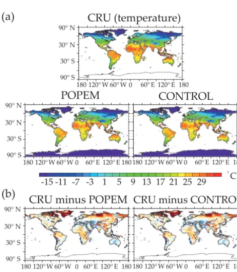
Figure 10 compares the annual mean temperatures for the period 1950–2000. CESM simulations show a signif-icant bias in high latitudes of the Northern Hemisphere (cf. Fig. 10a and b). In these areas, the model produces colder temperatures than those registered in the CRUTS reference data but this is also an issue in the CONTROL run. This de-viation is also apparent in Fig. 4b, where negative values lie away from the idealized regression line, and indicate further improvement of the CESM.
The bias is also reproduced when compared with tem-perature anomalies for a specific region. Thus, for instance, CESM gives poor scores in the Barents Sea area (Fig. 11a) while POPEM obtains better results for the Bering Sea, es-pecially in the Russian part (Fig. 11b). Here, POPEM gives more realistic values for the period 1970–1998 but, even with the improvement, the model still overestimates the tempera-ture anomaly.
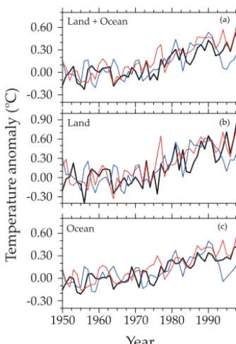
If we focus on global temperature anomalies, CESM sim-ulations are able to reproduce the progressive increase in the temperature anomaly (Fig. 12a). However, the CONTROL case simulates a sharp drop at the end of the period (1990– 1999), while POPEM portrays this change as smooth, in agreement with the observations.
The differences between CONTROL and POPEM are bet-ter demonstrated when comparing land and ocean separately (Fig. 12b and c). While the temperature anomalies for land are quite similar in both cases, POPEM provides a better rep-resentation of the ocean tendency from 1992 onwards, and that translates to an overall improvement (Fig. 12a).
3.3 Validation against ESPI and ONI indices
0 1 2 3 4 5 6 7 8 9 10 11 12 13 14 15 -0.9 -0.6 -0.3 0 0.3 0.6 0.9 180 120° W 60° W 0 60° E 120° E 180
POPEM
CONTROL CONTROL minus POPEM
30°N
30° S
90° S 90° N
º C
-12 -6 0 6 12 18 24 30
C
-1.8 -1.2 -0.6 0 0.6 1.2 1.8
T
emper
ature
Precipitation
(a)
(b)
mm day-1 mm day-1
30°N
30° S
90° S 90° N
180 120° W 60° W 0 60° E 120° E 180 180 120° W 60° W 0 60° E 120° E 180
180 120° W 60° W 0 60° E 120° E 180 180 120° W 60° W 0 60° E 120° E 180 180 120° W 60° W 0 60° E 120° E 180
Figure 6.A comparison of global annual mean precipitation (1950–2000) for the CONTROL and POPEM(a).(b)is a comparison of annual
mean surface temperatures. The maps in the right-hand column show the absolute differences between the simulations (CONTROL minus POPEM). In these, blues represent higher values in POPEM and reds represent higher values in the CONTROL.
(a)
(b)
GPCP (precipitation)
POPEM CONTROL
GPCP minus POPEM GPCP minus CONTROL
30° N
30° S
90° S 90° N
180 120° W 60° W 0 60° E 120° E 180
0 1 2 3 4 5 6 7 8 9 10
0 2 4 6
-2 -4 -6
mm day-1
mm day-1
30° N
30° S
90° S 90° N
180 120° W 60° W 0 60° E 120° E 180
30° N
30° S
90° S 90° N
180 120° W 60° W 0 60° E 120° E180
180 120° W 60° W 0 60° E 120° E 180
180120° W 60° W 0 60° E 120° E 180
Figure 7. A comparison of the global annual mean
precipita-tion (1980–2000) as simulated by the CESM (POPEM and CON-TROL) model and GPCP observational database. (a) Global an-nual mean precipitation maps for GPCP, POPEM, and CONTROL.
(b)Absolute difference maps. Units are in mm day−1.
30
20
10
Mean precipitation
GPCP CONTROL POPEM
0 2 4 6 8 10
2 4 6 8 10
2 4 6 8
Count
Count
Count
0 10 20 30 0
20
10
0 (a)
(b)
(c)
Figure 8.Histograms of the mean precipitation in the El Niño-4
GPCP CONTROL POPEM
Ja
n
Mar Ma y Jul
Sep Nov
7.0 4.0 3.0 2.0 6.0 5.0 (a) 8.0 4.0 2.0 0.0 Au g
Oct Dec Feb Apr Jun 6.0 (b) 12.0 6.0 3.0 0.0 Ja n Mar (c) Ma
y Jul Sep No v 9.0 P re ci p it at io n ( m m d ay -1)
Figure 9. Monthly precipitation (1980-1999) based on GPCP,
CONTROL, and POPEM for three of the regions with important bi-ases in CESM.(a)Shows precipitation for the area affected by the double-ITCZ bias in the Southern Hemisphere (20◦S–0 , 80◦E– 100◦W);(b)for the top end of Australia (30–10◦S, 128–140◦E); and (c)for the Tibetan Plateau (22–32◦N, 78–92◦W). The black line represents observations (GPCP), the blue line is the CONTROL case, and the red line is the POPEM case. Units are in mm day−1. The arrow indicates the improvement of the POPEM model.
(a)
(b)
CRU (temperature)
POPEM
CONTROL
CRU minus POPEM CRU minus CONTROL
30° N30° S
90° S 90° N
180 120° W 60° W 0 60° E 120° E 180
-15 -11 -7 -3 1 9 13 17 21 25 29
0 2 3 4
-2 -4 -6 C C 5 -1 1 -3
-5 5 6
30° N
30° S
90° S 90° N
180 120° W 60° W 0 60° E 120° E 180 180 120° W 60° W 0 60° E 120° E 180
180 120° W 60° W 0 60° E 120° E 180 180 120° W 60° W 0 60° E 120° E 180
30° N
30° S
90° S 90° N
Figure 10.A comparison of the annual mean temperature (1950–
2000) as simulated by the CESM model (POPEM and CONTROL) and CRU observational database.(a)Global annual mean tempera-ture maps for CRU, POPEM, and CONTROL.(b)Absolute differ-ence maps. Units are in◦C.
atmospheric circulation (Trenberth, 1997). Historically, the definition of ENSO does not include precipitation because of the limitations of stations (Ropelewski and Halpert, 1987), but recent work with satellites has confirmed that this phe-nomenon is a major driver of global precipitation variability (Haddad et al., 2004).
Barents Sea
Bering Sea (Russia)
Bering Sea (N. America)
GISTEMP CONTROL POPEM 1950 1960 1970 1980 1990 -3.0 0.0 1.0 3.0 -2.0 0.0 4.0 -2.0 -1.0 1.0 2.0 4.0
T
em
p
er
at
u
re
an
o
m
al
y
(
C
)
oYear
2.0 -4.0 3.0 0.0 4.0 2.0 -1.0 -2.0 (a) (b) (c)Figure 11.A comparison of the annual mean surface temperature
anomaly between GISTEMP, CONTROL, and POPEM from 1950 to 1999. (a) Represents the Barents Sea (68–80◦N, 19–68◦E);
(b)Russian part of the Bering Sea (50–65◦N, 150–180◦E); and
(c)American part of the Bering Sea (50–75◦N, 140–180◦W). The black line represents observational data (GISTEMP), the blue line is the CONTROL case, and the red is the POPEM case. Anomaly was referenced to 1951–1980 period.
A major advantage of satellite-derived precipitation in-dices over more conventional ones is the description of the strength and position of the Walker circulation (Cur-tis and Adler, 2000). Under that assumption, Cur(Cur-tis and Adler (2000) derived three satellite-based precipitation dices: the ENSO precipitation index (ESPI), El Niño in-dex (EI), and La Niña inin-dex (LI). Precipitation anomalies are averaged over areas of the equatorial Pacific and Maritime Continent – where the strongest precipitation anomalies as-sociated with ENSO are found – to construct differences or basin-wide gradients (Curtis, 2008).
Figure 13 shows a comparison of GPCP, CONTROL, and POPEM for the ESPI, EI, and LI indices.
Table 1.Comparison of the ONI index for the period 1950–1999. The table compares the ability of the models to reproduce the number, strength, and duration of El Niño events.
Source Number Agreement1 Disagreement2 Intensity Duration4avg
of events bias3avg
CPC 14 10.3
CONTROL 7 33 121 0.59◦C 19.4
POPEM 10 37 121 0.22◦C 11.4
1The number of months that CPC and CESM agree on El Niño.2Disagreement defined as the number of months where CPC and CESM obtain opposite results.3Intensity: (|CESM ONI| − |CPC ONI|)/number of cases (units in◦C).4Mean duration of El Niño event (in months).
Land + Ocean
Land
Ocean
GISTEMP CONTROL POPEM
1950 1960 1970 1980 1990 -0.30
0.00 0.30 0.60 -0.30 0.00 0.30 0.60
-0.30 0.00 0.30 0.60 0.90
T
em
p
er
at
u
re
an
o
m
al
y
(
C
)
o
Year
(a)
(b)
(c)
Figure 12.A comparison of the global annual mean surface
tem-perature anomaly between GISTEMP, CONTROL, and POPEM from 1950 to 1999.(a)Global,(b)land, and(c)ocean. The black line represents observational data (GISTEMP), the blue line is the CONTROL case, and the red is the POPEM case. Anomaly was referenced to 1951–1980 period.
Another widely used ENSO index is the Oceanic Niño Index (hereafter ONI). ONI was developed by the NOAA Climate Prediction Center (CPC) as the principal means for monitoring, assessing, and predicting ENSO (Kousky and Higgins, 2007). This index is defined as 3-month running-mean values of SST departures from the average in the Niño-3.4 region. It is computed from a set of homogeneous histor-ical SST analyses (Kousky and Higgins, 2007; Smith et al., 2003).
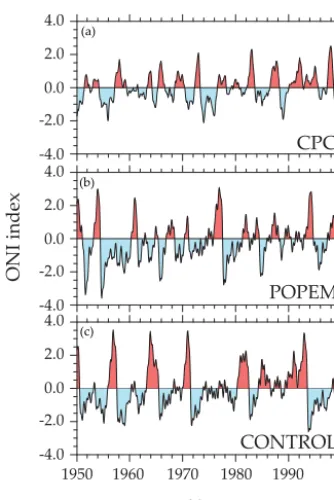
Figure 14 compares the ONI index for CPC, POPEM, and CONTROL cases. It is clear from the figure that POPEM pro-duces a more realistic representation of the ENSO, especially
1979 1983 1987 1991 1995 1999
GPCP CONTROL POPEM
-4.0 -2.0 0.0 2.0 4.0
ESPI index
Year
-4.0 -2.0 0.0 2.0 4.0
EI
-4.0 -2.0 0.0 2.0 4.0
LI
(a)
(b)
(c)
Figure 13.Time series of precipitation anomalies for the ENSO
region after Curtis and Adler (2000).(a)ENSO precipitation in-dex (ESPI),(b) El Niño Index (EI), and(c)La Niña Index (LI). The Black line shows GPCP data, the blue line is the CONTROL case, and the red line is the POPEM case. Orange shading denotes El Niño years defined as consecutive months (minimum 3) with NIÑO3.4 SST anomalies (5◦N–5◦S, 170–120◦W) greater than +0.5◦C.
if we focus on the 1992–1999 period. POPEM also obtains better results than CONTROL in the number of simulated El Niño events (see Table 1). The improvement is also notice-able in the intensity. The CONTROL case exhibits an overly strong ENSO – a common bias in CESM (Tang et al., 2016) – but POPEM reduces this bias (0.22◦C versus 0.59◦C).
1950 1960 1970 1980 1990 -2.0
0.0 4.0
2.0
-4.0 -2.0 0.0 4.0
2.0
-4.0
-2.0 0.0 4.0
2.0
-4.0
ONI index
Year
CPC
POPEM
CONTROL (a)
(b)
(c)
Figure 14.Comparison of the Oceanic El Niño Index (ONI) for
CPC (a), POPEM (b), and CONTROL (c) cases. El Niño and La Niña are defined according to Kousky and Higgins (2007): 3-month running mean with anomalies greater than +0.5◦C (or −0.5◦C) for at least 5 consecutive months in the NIÑO3.4 region. The base period for computing SST departures is 1971–1999.
4 Conclusions and future work
Like all models, climate models are simplified versions of the real world and therefore do not include the full complexity of the Earth system. Due to certain limitations, e.g., compu-tational resources or spatial and temporal resolution, climate models have to make assumptions and resort to parameteri-zations.
One important simplification is to use prescribed forcings instead of dynamically modeling GHG emissions. However, precise modeling of anthropogenic CO2emissions is impor-tant for climate change research as it allows sensitivity anal-yses to be performed.
Here we present a new module of gridded CO2 emis-sions that is coupled with CESM. The module, denominated POPEM, computes anthropogenic CO2 emissions by using population estimates as a proxy for disaggregating emissions beyond the national level. POPEM makes CESM use dynam-ical emission data instead of fixed concentration parameters. In terms of population and emissions, the module com-pares well when validated with data. Thus, POPEM’s esti-mates for the 1950–2000 period are in general agreement with population and emission inventories from the recent past. In spite of the more realistic depiction of the actual emissions (Fig. 3), issues persist. The performance of the model can be further improved in places where
popula-tion projecpopula-tions are difficult to model. For instance, POPEM tends to underestimate emissions on the west coast of the United States and the Anatolian Plateau, and overestimates emissions in China and Japan.
When the POPEM module is coupled with CESM to gen-erate climatologies, the ability to successfully model pre-cipitation and surface temperature is preserved. Moreover, the results of 50-year simulations show that the dynami-cal modeling of emissions produced by POPEM results in slight but noticeable differences in the resultant precipitation regime and surface temperature. Thus, dynamically model-ing the emissions alters the ITCZ by reducmodel-ing precipitation in the Southern Hemisphere and increasing it in the North-ern Hemisphere. For particularly interesting areas, such as the El Niño-4 region, the POPEM outperforms the traditional approach.
Further work will be devoted to improving the modeling of those areas and hopefully minimizing some of the original biases of the CESM model. These include the emergence of a double ITCZ in CESM simulations, which is a common bias for most climate models (Oueslati and Bellon, 2015), as well as SST simulated by climate models, which are generally too low in the Northern Hemisphere and too high in the Southern Hemisphere (Wang et al., 2014).
Current applications of the parameterization include eval-uating the effects of changes in regional policies, and a bet-ter understanding of the carbon cycle (Friedlingstein et al., 2006). Future work will be devoted to evaluating the climate response to alternative anthropogenic CO2emissions, to cou-pling POPEM with the newest version of CESM (CESM2; Joel, 2018), to fully coupling human–Earth subsystems, to increasing the spatial resolution of the simulations, and to refining the spatial and temporal distribution of emission es-timates.
Although the version of POPEM presented here is al-ready functional, this work is intended to be just the first step in fully coupling socioeconomic dynamics with ESMs. This will include bidirectional feedbacks between human and Earth systems and the simulation of societal processes based on the internal dynamics of the model instead of using ex-ternal sources to make the projections. Only within a cou-pled global human–Earth system framework can we produce more realistic representations of the Earth system capturing much of the important feedbacks that are missing from cur-rent models (Motesharrei et al., 2016). The success of this approach will depend on the ability of scientists from differ-ent research fields to work in an interdisciplinary framework of continuous collaboration.
Data availability. Code (POPEM) and model outputs
2018). Climate Research Unit Time Series (CRUTS) data are avail-able at https://crudata.uea.ac.uk/cru/data/hrg/ (last access: 30 July 2018; Harris et al., 2014). GISTEMP data are available at the NASA Goddard Institute for Space Studies website (https://data. giss.nasa.gov/gistemp/, last access: 30 July 2018; Hansen et al., 2010). The Oceanic Niño Index (ONI) is produced by the Climate Prediction Center and is accessible at http://origin.cpc.ncep.noaa. gov/products/analysis_monitoring/ensostuff/ONI_v5.php (last ac-cess: 30 July 2018; Kousky and Higgins, 2007).
Supplement. The supplement related to this article is available
online at: https://doi.org/10.5194/esd-9-1045-2018-supplement.
Author contributions. AN and FJT contributed to the experiment
design, coding, analysis, manuscript writing, and made the amend-ments suggested by the referees. RM contributed to manuscript writing and POPEM-CESM implementation in the University of Castilla–La Mancha supercomputing center.
Competing interests. The authors declare that they have no
con-flict of interest.
Acknowledgements. Funding from projects CGL2013-48367-P,
CGL2016-80609-R (Ministerio de Economía y Competitividad, Ciencia e Innovación) is gratefully acknowledged. Andrés Navarro acknowledges support from grant FPU 13/02798 for carrying out his PhD. We want to thank the five referees for their constructive comments and recommendations. Their comments have greatly improved the manuscript.
Edited by: Yun Liu
Reviewed by: Svetla Hristova-Veleva and four anonymous referees
References
Adler, R., Sapiano, M., Huffman, G., Bolvin, D., Wang, J.-J., Gu, G., Nelkin, E., Xie, P., Chiu, L., Ferraro, R., Schneider, U., and Becker, A.: New Global Precipitation Climatology Project monthly analysis product corrects satellite data shifts, GEWEX News, 26, 7–9, 2016.
Adler, R. F., Sapiano, M. R. P., Huffman, G. J., Wang, J.-J., Gu, G., Bolvin, D., Chiu, L., Schneider, U., Becker, A., Nelkin, E., Xie, P., Ferraro, R., and Shin, D.-B: The Global Precipitation Cli-matology Project (GPCP) Monthly Analysis (New Version 2.3) and a Review of 2017 Global Precipitation, Atmosphere, 9, 138, https://doi.org/10.3390/atmos9040138, 2018 (data available at: http://gpcp.umd.edu/, last access: 30 July 2018).
Alter, R. E., Douglas, H. C., Winter, J. M., and Eltahir, E. A. B.: 20th-century regional climate change in the central United States attributed to agricultural intensification, Geophys. Res. Lett., 45, 1586–1594, https://doi.org/10.1002/2017GL075604, 2018. Andres, R. J., Marland, G., Fung, I. and Matthews, E.: A 1◦×1◦
dis-tribution of carbon dioxide emissions from fossil fuel
consump-tion and cement manufacture, 1950–1990, Global Biogeochem. Cy., 10, 419–429, https://doi.org/10.1029/96GB01523, 1996. Andres, R. J., Boden, T. A., and Higdon, D. M.: Gridded
uncertainty in fossil fuel carbon dioxide emission maps, a CDIAC example, Atmos. Chem. Phys., 16, 14979–14995, https://doi.org/10.5194/acp-16-14979-2016, 2016.
Archer, D., Eby, M., Brovkin, V., Ridgwell, A., Cao, L., Mikola-jewicz, U., Caldeira, K., Matsumoto, K., Munhoven, G., Mon-tenegro, A., and Tokos, K.: Atmospheric Lifetime of Fossil Fuel Carbon Dioxide, Annu. Rev. Earth Planet. Sci., 37, 117–134, https://doi.org/10.1146/annurev.earth.031208.100206, 2009. Ashok, K. and Yamagata, T.: Climate change: The El N˜ıo with a
dif-ference, Nature, 461, 481–484, https://doi.org/10.1038/461481a, 2009.
Ashok, K., Behera, S. K., Rao, S. A., Weng, H., and Yamagata, T.: El Niño Modoki and its possible
tele-connection, J. Geophys. Res.-Oceans, 112, C11007,
https://doi.org/10.1029/2006JC003798, 2007.
Bacmeister, J. T., Wehner, M. F., Neale, R. B., Gettelman, A., Han-nay, C., Lauritzen, P. H., Caron, J. M., and Truesdale, J. E.: Exploratory high-resolution climate simulations using the com-munity atmosphere model (CAM), J. Climate, 27, 3073–3099, https://doi.org/10.1175/JCLI-D-13-00387.1, 2014.
Baker, N. C. and Taylor, P. C.: A Framework for Evaluating Cli-mate Model Performance Metrics, J. CliCli-mate, 29, 1773–1782, https://doi.org/10.1175/JCLI-D-15-0114.1, 2016.
Barnett, T. P., Pierce, D. W., Hidalgo, H. G., Bonfils, C., Santer, B. D., Das, T., Bala, G., Wood, A. W., Nozawa, T., Mirin, A. A., Cayan, D. R., and Dettinger, M. D.: Human-induced changes in the hydrology of the Western United States, Science, 319, 1080– 1083, https://doi.org/10.1126/science.1152538, 2008.
Baumberger, C., Knutti, R., and Hirsch Hadorn, G.: Building confidence in climate model projections: an analysis of infer-ences from fit, Wiley Interdiscip. Rev. Clim. Change, 8, e454, https://doi.org/10.1002/wcc.454, 2017.
Bentsen, M., Bethke, I., Debernard, J. B., Iversen, T., Kirkevåg, A., Seland, Ø., Drange, H., Roelandt, C., Seierstad, I. A., Hoose, C., and Kristjánsson, J. E.: The Norwegian Earth Sys-tem Model, NorESM1-M – Part 1: Description and basic evalu-ation of the physical climate, Geosci. Model Dev., 6, 687–720, https://doi.org/10.5194/gmd-6-687-2013, 2013.
Boden, T. A., Marland, G., and Andres, R.: Global, Regional, and National Fossil-Fuel CO2Emissions, Carbon Dioxide Inf. Anal.
Center, Oak Ridge Natl. Lab., U.S. Dep. Energy, Oak Ridge, Tenn., USA, https://doi.org/10.3334/CDIAC/00001_V2017, 2017.
Boville, B. A. and Gent, P. R.: The NCAR
cli-mate system model, version one, J. Climate,
11, 1115–1130,
https://doi.org/10.1175/1520-0442(1998)011<1115:TNCSMV>2.0.CO;2, 1998.
Brown, P. T., Li, W., Cordero, E. C., and Mauget, S. A.: Comparing the model-simulated global warming signal to observations using empirical estimates of unforced noise, Sci. Rep.-UK, 5, 9957, https://doi.org/10.1038/srep09957, 2015.
Christensen, J. H. and Boberg, F.: Temperature dependent climate projection deficiencies in CMIP5 models, Geophys. Res. Lett., 39, L24705, https://doi.org/10.1029/2012GL053650, 2012. Collins, W. D., Bitz, C. M., Blackmon, M. L., Bonan, G. B.,
Bretherton, C. S., Carton, J. A., Chang, P., Doney, S. C., Hack, J. J., Henderson, T. B., Kiehl, J. T., Large, W. G., McKenna, D. S., Santer, B. D., and Smith, R. D.: The Community Climate System Model version 3 (CCSM3), J. Climate, 19, 2122–2143, https://doi.org/10.1175/JCLI3761.1, 2006.
Craig, A. P., Vertenstein, M., and Jacob, R.: A new flexible cou-pler for earth system modeling developed for CCSM4 and CESM1, Int. J. High Perform. Comput. Appl., 26, 31–42, https://doi.org/10.1177/1094342011428141, 2012.
Crutzen, P. J.: Geology of mankind, Nature, 415, p. 23, https://doi.org/10.1038/415023a, 2002.
Curtis, S.: The El Niño–Southern Oscillation and
Global Precipitation, Geogr. Compass, 2, 600–619,
https://doi.org/10.1111/j.1749-8198.2008.00105.x, 2008. Curtis, S., Adler, R., Curtis, S., and Adler, R.: ENSO
Indices Based on Patterns of Satellite-Derived Precipita-tion, J. Climate, 13, 2786–2793, https://doi.org/10.1175/1520-0442(2000)013<2786:EIBOPO>2.0.CO;2, 2000.
Dai, A.: Precipitation characteristics in eighteen
cou-pled climate models, J. Climate, 19, 4605–4630,
https://doi.org/10.1175/JCLI3884.1, 2006.
Davey, M., Huddleston, M., Sperber, K., Braconnot, P., Bryan, F., Chen, D., Colman, R., Cooper, C., Cubasch, U., Delecluse, P., DeWitt, D., Fairhead, L., Flato, G., Gordon, C., Hogan, T., Ji, M., Kimoto, M., Kitoh, A., Knutson, T., Latif, M., Le Treut, H., Li, T., Manabe, S., Mechoso, C., Meehl, G., Power, S., Roeck-ner, E., Terray, L., Vintzileos, A., Voss, R., Wang, B., Wash-ington, W., Yoshikawa, I., Yu, J., Yukimoto, S., and Zebiak, S.: STOIC: A study of coupled model climatology and vari-ability in tropical ocean regions, Clim. Dynam., 18, 403–420, https://doi.org/10.1007/s00382-001-0188-6, 2002.
Edwards, P. N.: History of climate modeling, Wiley Interdiscip. Rev. Clim. Change, 2, 128–139, https://doi.org/10.1002/wcc.95, 2011.
Eyring, V., Bony, S., Meehl, G. A., Senior, C. A., Stevens, B., Stouffer, R. J., and Taylor, K. E.: Overview of the Coupled Model Intercomparison Project Phase 6 (CMIP6) experimen-tal design and organization, Geosci. Model Dev., 9, 1937–1958, https://doi.org/10.5194/gmd-9-1937-2016, 2016.
Flato, G. M.: Earth system models: an overview,
Wi-ley Interdiscip. Rev. Clim. Change, 2, 783–800,
https://doi.org/10.1002/wcc.148, 2011.
Fogli, P. G. and Iovino, D.: CMCC–CESM–NEMO: Toward the new CMCC Earth System Model, C. Res. Rep. RP0248, available at: http://www.cmcc.it/wp-content/uploads/2015/02/ rp0248-ans-12-2014.pdf (last access: 10 May 2018), 2014. Friedlingstein, P., Cox, P., Betts, R., Bopp, L., von Bloh, W.,
Brovkin, V., Cadule, P., Doney, S., Eby, M., Fung, I., Bala, G., John, J., Jones, C., Joos, F., Kato, T., Kawamiya, M., Knorr, W., Lindsay, K., Matthews, H. D., Raddatz, T., Rayner, P., Reick, C., Roeckner, E., Schnitzler, K. G., Schnur, R., Strassmann, K., Weaver, A. J., Yoshikawa, C., and Zeng, N.: Climate-carbon cycle feedback analysis: Results from the C4MIP model intercomparison, J. Climate, 19, 3337–3353, https://doi.org/10.1175/JCLI3800.1, 2006.
Gately, C. K., Hutyra, L. R., Wing, I. S., and Brondfield, M. N.: A bottom up approach to on-road CO2 emissions
estimates: Improved spatial accuracy and applications for regional planning, Environ. Sci. Technol., 47, 2423–2430, https://doi.org/10.1021/es304238v, 2013.
Gent, P. R., Danabasoglu, G., Donner, L. J., Holland, M. M., Hunke, E. C., Jayne, S. R., Lawrence, D. M., Neale, R. B., Rasch, P. J., Vertenstein, M., Worley, P. H., Yang, Z. L., and Zhang, M.: The community climate system model version 4, J. Climate, 24, 4973–4991, https://doi.org/10.1175/2011JCLI4083.1, 2011. Giorgetta, M. A., Jungclaus, J., Reick, C. H., Legutke, S., Bader,
J., Böttinger, M., Brovkin, V., Crueger, T., Esch, M., Fieg, K., Glushak, K., Gayler, V., Haak, H., Hollweg, H.-D., Ilyina, T., Kinne, S., Kornblueh, L., Matei, D., Mauritsen, T., Mikolajew-icz, U., Mueller, W., Notz, D., Pithan, F., Raddatz, T., Rast, S., Redler, R., Roeckner, E., Schmidt, H., Schnur, R., Segschnei-der, J., Six, K. D., Stockhause, M., Timmreck, C., Wegner, J., Widmann, H., Wieners, K.-H., Claussen, M., Marotzke, J., and Stevens, B.: Climate and carbon cycle changes from 1850 to 2100 in MPI-ESM simulations for the Coupled Model Inter-comparison Project phase 5, J. Adv. Model. Earth Syst., 5, 572– 597, https://doi.org/10.1002/jame.20038, 2013.
Grandey, B. S., Cheng, H., and Wang, C.: Transient cli-mate impacts for scenarios of aerosol emissions from Asia: A story of coal versus gas, J. Climate, 29, 2849–2867, https://doi.org/10.1175/JCLI-D-15-0555.1, 2016.
Guo, L., Highwood, E. J., Shaffrey, L. C., and Turner, A. G.: The effect of regional changes in anthropogenic aerosols on rainfall of the East Asian Summer Monsoon, Atmos. Chem. Phys., 13, 1521–1534, https://doi.org/10.5194/acp-13-1521-2013, 2013. Gurney, K. R., Mendoza, D. L., Zhou, Y., Fischer, M. L., Miller,
C. C., Geethakumar, S., and de la Rue du Can, S.: High Resolution Fossil Fuel Combustion CO2 Emission Fluxes for
the United States, Environ. Sci. Technol., 43, 5535–5541, https://doi.org/10.1021/es900806c, 2009.
Haddad, Z. S., Meagher, J. P., Adler, R. F., Smith, E. A., Im, E., and Durden, S. L.: Global variability of precipitation according to the Tropical Rainfall Measuring Mission, J. Geophys. Res.-Atmos., 109, D17103, https://doi.org/10.1029/2004JD004607, 2004. Hansen, J. and Lebedeff, S.: Global trends of measured
sur-face air temperature, J. Geophys. Res., 92, 13345–13372, https://doi.org/10.1029/JD092iD11p13345, 1987.
Hansen, J., Ruedy, R., Sato, M., and Reynolds, R.: Global surface air temperature in 1995: Return to pre-Pinatubo level, Geophys. Res. Lett., 23, 1665–1668, https://doi.org/10.1029/96GL01040, 1996.
Hansen, J., Ruedy, R., Sato, M., and Lo, K.: Global
sur-face temperature change, Rev. Geophys., 48, RG4004,
https://doi.org/10.1029/2010RG000345, 2010 (data avail-able at: https://data.giss.nasa.gov/gistemp/, last access: 30 July 2018).
Hao, Z., AghaKouchak, A., and Phillips, T. J.: Changes in concurrent monthly precipitation and temperature extremes, Environ. Res. Lett., 8, 34014, https://doi.org/10.1088/1748-9326/8/3/034014, 2013.
Hargreaves, J. C. and Annan, J. D.: Can we trust climate models?, Wiley Interdiscip. Rev. Clim. Change, 5, 435–440, https://doi.org/10.1002/wcc.288, 2014.
Harris, I., Jones, P. D., Osborn, T. J. and Lister, D. H.: Up-dated high-resolution grids of monthly climatic observations – the CRU TS3.10 Dataset, Int. J. Climatol., 34, 623–642, https://doi.org/10.1002/joc.3711, 2014 (data available at: https: //crudata.uea.ac.uk/cru/data/hrg/, ast access: 30 July 2018). Hou, A. Y., Kakar, R. K., Neeck, S., Azarbarzin, A. A.,
Kum-merow, C. D., Kojima, M., Oki, R., Nakamura, K., and Iguchi, T.: The global precipitation measurement mission, B. Am. Me-teorol. Soc., 95, 701–722, https://doi.org/10.1175/BAMS-D-13-00164.1, 2014.
Hourdin, F., Mauritsen, T., Gettelman, A., Golaz, J.-C., Balaji, V., Duan, Q., Folini, D., Ji, D., Klocke, D., Qian, Y., Rauser, F., Rio, C., Tomassini, L., Watanabe, M., and Williamson, D.: The Art and Science of Climate Model Tuning, B. Am. Me-teorol. Soc., 98, 589–602, https://doi.org/10.1175/BAMS-D-15-00135.1, 2017.
Huang, X. and Ullrich, P. A.: Irrigation impacts on California’s cli-mate with the variable-resolution CESM, J. Adv. Model. Earth Syst., 8, 1151–1163, https://doi.org/10.1002/2016MS000656, 2016.
Hunke, E. C. and Lipscomb, W. H.: CICE: the Los Alamos sea ice model user’s manual, version 4, Tech. Rep., Los Alamos National Laboratory, available at: https://www.osti.gov/scitech/ biblio/1364126 (last access: 20 February 2018), 2008.
Hurrell, J. W., Holland, M. M., Gent, P. R., Ghan, S., Kay, J. E., Kushner, P. J., Lamarque, J.-F. F., Large, W. G., Lawrence, D., Lindsay, K., Lipscomb, W. H., Long, M. C., Mahowald, N., Marsh, D. R., Neale, R. B., Rasch, P., Vavrus, S., Vertenstein, M., Bader, D., Collins, W. D., Hack, J. J., Kiehl, J., and Mar-shall, S.: The Community Earth System Model: A Framework for Collaborative Research, B. Am. Meteorol. Soc., 94, 1339– 1360, https://doi.org/10.1175/BAMS-D-12-00121.1, 2013. Hwang, Y.-T. and Frierson, D. M. W.: Link between the
double-Intertropical Convergence Zone problem and cloud biases over the Southern Ocean, P. Natl. Acad. Sci. USA, 110, 4935–4940, https://doi.org/10.1073/pnas.1213302110, 2013.
IPCC: Climate Change 2013 – The Physical Science Basis, edited by: Intergovernmental Panel on Climate Change, Cambridge University Press, Cambridge, 2014a.
IPCC: Climate Change 2014: Synthesis Report. Contribution of Working Groups I, II and III to the Fifth Assessment Report of the Intergovernmental Panel on Climate Change, edited by: Pachauri, R. K. and Meyer, L. A., Geneva, Switzerland, 151 pp., 2014b.
Joel, L.: New version of popular climate model released, EOS, 99, https://doi.org/10.1029/2018EO101489, 2018.
Justin Small, R., Curchitser, E., Hedstrom, K., Kauffman, B., and Large, W. G.: The Benguela upwelling system: Quanti-fying the sensitivity to resolution and coastal wind represen-tation in a global climate model, J. Climate, 28, 9409–9432, https://doi.org/10.1175/JCLI-D-15-0192.1, 2015.
Kay, J. E., Deser, C., Phillips, A., Mai, A., Hannay, C., Strand, G., Arblaster, J. M., Bates, S. C., Danabasoglu, G., Edwards, J., Holland, M., Kushner, P., Lamarque, J. F., Lawrence, D., Lindsay, K., Middleton, A., Munoz, E., Neale, R., Oleson, K., Polvani, L., and Vertenstein, M.: The community earth
sys-tem model (CESM) large ensemble project: A community re-source for studying climate change in the presence of inter-nal climate variability, B. Am. Meteorol. Soc., 96, 1333–1349, https://doi.org/10.1175/BAMS-D-13-00255.1, 2015.
Kerbyson, D. J. and Jones, P. W.: A Performance Model of the Par-allel Ocean Program, Int. J. High Perform. Comput. Appl., 19, 261–276, https://doi.org/10.1177/1094342005056114, 2005. Kidd, C., Becker, A., Huffman, G. J., Muller, C. L., Joe, P.,
Skofronick-Jackson, G., and Kirschbaum, D. B.: So, how much of the Earth’s surface is covered by rain gauges?, B. Am. Meteorol. Soc., 98, 69–78, https://doi.org/10.1175/BAMS-D-14-00283.1, 2017.
Kousky, V. E. and Higgins, R. W.: An Alert Classification System for Monitoring and Assessing the ENSO Cycle, Weather Fore-cast., 22, 353–371, https://doi.org/10.1175/WAF987.1, 2007 (data available at: http://origin.cpc.ncep.noaa.gov/products/ analysis_monitoring/ensostuff/ONI_v5.php, last access: 30 July 2018).
Ladyman, J., Lambert, J., and Wiesner, K.: What is
a complex system?, Eur. J. Philos. Sci., 3, 33–67,
https://doi.org/10.1007/s13194-012-0056-8, 2013.
Lahsen, M.: Seductive Simulations? Uncertainty Distribution Around Climate Models, Soc. Stud. Sci., 35, 895–922, https://doi.org/10.1177/0306312705053049, 2005.
Lawrence, D. M., Oleson, K. W., Flanner, M. G., Thornton, P. E., Swenson, S. C., Lawrence, P. J., Zeng, X., Yang, Z.-L., Levis, S., Sakaguchi, K., Bonan, G. B., and Slater, A. G.: Parameter-ization improvements and functional and structural advances in Version 4 of the Community Land Model, J. Adv. Model. Earth Syst., 3, M03001, https://doi.org/10.1029/2011MS00045, 2011. Lehner, F., Joos, F., Raible, C. C., Mignot, J., Born, A., Keller, K.
M., and Stocker, T. F.: Climate and carbon cycle dynamics in a CESM simulation from 850 to 2100 CE, Earth Syst. Dynam., 6, 411–434, https://doi.org/10.5194/esd-6-411-2015, 2015. Levis, S., Gordon, B. B., Erik Kluzek, Thornton, P. E., Jones, A.,
Sacks, W. J., and Kucharik, C. J.: Interactive Crop Management in the Community Earth System Model (CESM1): Seasonal in-fluences on land-atmosphere fluxes, J. Climate, 25, 4839–4859, https://doi.org/10.1175/JCLI-D-11-00446.1, 2012.
Li, G. and Xie, S. P.: Tropical biases in CMIP5 multi-model ensemble: The excessive equatorial pacific cold tongue and double ITCZ problems, J. Climate, 27, 1765–1780, https://doi.org/10.1175/JCLI-D-13-00337.1, 2014.
Lindsay, K., Bonan, G. B., Doney, S. C., Hoffman, F. M., Lawrence, D. M., Long, M. C., Mahowald, N. M., Keith Moore, J., Rander-son, J. T., Thornton, P. E., Lindsay, K., Bonan, G. B., Doney, S. C., Hoffman, F. M., Lawrence, D. M., Long, M. C., Ma-howald, N. M., Moore, J. K., Randerson, J. T., and Thornton, P. E.: Preindustrial-Control and Twentieth-Century Carbon Cy-cle Experiments with the Earth System Model CESM1(BGC), J. Climate, 27, 8981–9005, https://doi.org/10.1175/JCLI-D-12-00565.1, 2014.
Liu, X., Easter, R. C., Ghan, S. J., Zaveri, R., Rasch, P., Shi, X., Lamarque, J. F., Gettelman, A., Morrison, H., Vitt, F., Conley, A., Park, S., Neale, R., Hannay, C., Ekman, A. M. L., Hess, P., Mahowald, N., Collins, W., Iacono, M. J., Bretherton, C. S., Flan-ner, M. G., and Mitchell, D.: Toward a minimal representation of aerosols in climate models: Description and evaluation in the Community Atmosphere Model CAM5, Geosci. Model Dev., 5, 709–739, https://doi.org/10.5194/gmd-5-709-2012, 2012. Liu, Z., Mehran, A., Phillips, T. J., and AghaKouchak, A.: Seasonal
and regional biases in CMIP5 precipitation simulations, Clim. Res., 60, 35–50, https://doi.org/10.3354/cr01221, 2014.
Lorenz, E. N.: Deterministic Nonperiodic Flow, J.
At-mos. Sci., 20, 130–141,
https://doi.org/10.1175/1520-0469(1963)020<0130:DNF>2.0.CO;2, 1963.
Martin, G. M., Bellouin, N., Collins, W. J., Culverwell, I. D., Hal-loran, P. R., Hardiman, S. C., Hinton, T. J., Jones, C. D., Mc-Donald, R. E., McLaren, A. J., O’Connor, F. M., Roberts, M. J., Rodriguez, J. M., Woodward, S., Best, M. J., Brooks, M. E., Brown, A. R., Butchart, N., Dearden, C., Derbyshire, S. H., Dharssi, I., Doutriaux-Boucher, M., Edwards, J. M., Falloon, P. D., Gedney, N., Gray, L. J., Hewitt, H. T., Hobson, M., Hud-dleston, M. R., Hughes, J., Ineson, S., Ingram, W. J., James, P. M., Johns, T. C., Johnson, C. E., Jones, A., Jones, C. P., Joshi, M. M., Keen, A. B., Liddicoat, S., Lock, A. P., Maidens, A. V., Manners, J. C., Milton, S. F., Rae, J. G. L., Ridley, J. K., Sel-lar, A., Senior, C. A., Totterdell, I. J., Verhoef, A., Vidale, P. L., and Wiltshire, A.: The HadGEM2 family of Met Office Unified Model climate configurations, Geosci. Model Dev., 4, 723–757, https://doi.org/10.5194/gmd-4-723-2011, 2011.
Mauritsen, T., Stevens, B., Roeckner, E., Crueger, T., Esch,
M., Giorgetta, M., Haak, H., Jungclaus, J., Klocke,
D., Matei, D., Mikolajewicz, U., Notz, D., Pincus, R., Schmidt, H., and Tomassini, L.: Tuning the climate of a global model, J. Adv. Model. Earth Syst., 4, M00A01, https://doi.org/10.1029/2012MS000154, 2012.
McPhaden, M. J., Zebiak, S. E.. and Glantz, M. H.: ENSO as an Integrating Concept in Earth Science, Science, 314, 1740–1745, https://doi.org/10.1126/science.1132588, 2006.
Mechoso, C. R., Robertson, A. W., Barth, N., Davey, M. K., Delecluse, P., Gent, P. R., Ineson, S., Kirtman, B., Latif, M., Treut, H. Le, Nagai, T., Neelin, J. D., Phi-lander, S. G. H., Polcher, J., Schopf, P. S., Stockdale, T., Suarez, M. J., Terray, L., Thual, O., and Tribbia, J. J.: The Seasonal Cycle over the Tropical Pacific in Cou-pled Ocean–Atmosphere General Circulation Models, Mon. Weather Rev., 123, 2825–2838, https://doi.org/10.1175/1520-0493(1995)123<2825:TSCOTT>2.0.CO;2, 1995.
Meehl, G. A. and Arblaster, J. M.: The Asian-Australian monsoon and El Nino–Southern Oscillation in the NCAR climate system model, J. Climate, 11, 1356–1385, https://doi.org/10.1175/1520-0442(1998)011<1356:TAAMAE>2.0.CO;2, 1998.
Meehl, G. A., Arblaster, J. M., Caron, J. M., Annamalai, H., Jochum, M., Chakraborty, A., and Murtugudde, R.: Monsoon regimes and processes in CCSM4. Part I: The
Asian-Australian monsoon, J. Climate, 25, 2583–2608,
https://doi.org/10.1175/JCLI-D-11-00184.1, 2012.
Monier, E., Scott, J. R., Sokolov, A. P., Forest, C. E., and Schlosser, C. A.: An integrated assessment modeling framework for un-certainty studies in global and regional climate change: The
MIT IGSM-CAM (version 1.0), Geosci. Model Dev., 6, 2063– 2085, https://doi.org/10.5194/gmd-6-2063-2013, 2013.
Moss, R. H., Edmonds, J. A., Hibbard, K. A., Manning, M. R., Rose, S. K., van Vuuren, D. P., Carter, T. R., Emori, S., Kainuma, M., Kram, T., Meehl, G. A., Mitchell, J. F. B., Nakicenovic, N., Ri-ahi, K., Smith, S. J., Stouffer, R. J., Thomson, A. M., Weyant, J. P., and Wilbanks, T. J.: The next generation of scenarios for climate change research and assessment, Nature, 463, 747–56, https://doi.org/10.1038/nature08823, 2010.
Motesharrei, S., Rivas, J., and Kalnay, E.: Human and nature dy-namics (HANDY): Modeling inequality and use of resources in the collapse or sustainability of societies, Ecol. Econ., 101, 90– 102, https://doi.org/10.1016/j.ecolecon.2014.02.014, 2014. Motesharrei, S., Rivas, J., Kalnay, E., Asrar, G. R., Busalacchi,
A. J., Cahalan, R. F., Cane, M. A., Colwell, R. R., Feng, K., Franklin, R. S., Hubacek, K., Miralles-Wilhelm, F., Miyoshi, T., Ruth, M., Sagdeev, R., Shirmohammadi, A., Shukla, J., Sre-bric, J., Yakovenko, V. M., and Zeng, N.: Modeling Sustain-ability: Population, Inequality, Consumption, and Bidirectional Coupling of the Earth and Human Systems, Natl. Sci. Rev., 3, nww081, https://doi.org/10.1093/nsr/nww081, 2016.
Müller-Hansen, F., Schlüter, M., Mäs, M., Hegselmann, R., Donges, J. F., Kolb, J. J., Thonicke, K., and Heitzig, J.: How to represent human behavior and decision making in Earth system models? A guide to techniques and approaches, Earth Syst. Dyn. Discuss., https://doi.org/10.5194/esd-2017-18, in review, 2017.
Nasrollahi, N., Aghakouchak, A., Cheng, L., Damberg, L., Phillips, T. J., Miao, C., Hsu, K., and Sorooshian, S.: How well do CMIP5 climate simulations replicate historical trends and patterns of meteorological droughts?, Water Resour. Res., 51, 2847–2864, https://doi.org/10.1002/2014WR016318, 2015.
Navarro, A., Moreno, R., Jiménez-Alcázar, A., and Tapi-ador, F. J.: Coupling population dynamics with earth sys-tem models: the POPEM model, Environ. Sci. Pollut. Res., https://doi.org/10.1007/s11356-017-0127-7, in press, 2017. Neale, R. B., Chen, C., Lauritzen, P. H., Williamson, D. L.,
Con-ley, A. J., Smith, A. K., Mills, M., and Morrison, H.: Description of the NCAR Community Atmosphere Model (CAM5.0), avail-able at: https://www.ccsm.ucar.edu/models/ccsm4.0/cam/docs/ description/cam4_desc.pdf (last access: 20 February 2018), 2012.
Neely, R. R., Conley, A. J., Vitt, F., and Lamarque, J. F.: A con-sistent prescription of stratospheric aerosol for both radiation and chemistry in the Community Earth System Model (CESM1), Geosci. Model Dev., 9, 2459–2470, https://doi.org/10.5194/gmd-9-2459-2016, 2016.
Nevison, C., Hess, P., Riddick, S., and Ward, D.: Denitrifica-tion, leaching, and river nitrogen export in the Community Earth System Model, J. Adv. Model. Earth Syst., 8, 272–291, https://doi.org/10.1002/2015MS000573, 2016.
New, M., Hulme, M., and Jones, P.: Representing twentieth-century space-time climate variability. Part I: Develop-ment of a 1961-90 mean monthly terrestrial climatol-ogy, J. Climate, 12, 829–856, https://doi.org/10.1175/1520-0442(1999)012<0829:RTCSTC>2.0.CO;2, 1999.
New, M., Hulme, M., Jones, P., New, M., Hulme, M.,
and Jones, P.: Representing Twentieth-Century Space–
Time Climate Variability. Part II: Development of 1901–
Climate, 13, 2217–2238, https://doi.org/10.1175/1520-0442(2000)013<2217:RTCSTC>2.0.CO;2, 2000.
Nobre, C., Brasseur, G. P., Shapiro, M. A., Lahsen, M., Brunet, G., Busalacchi, A. J., Hibbard, K., Seitzinger, S., Noone, K., Ometto, J. P., Nobre, C., Brasseur, G. P., Shapiro, M. A., Lah-sen, M., Brunet, G., Busalacchi, A. J., Hibbard, K., Seitzinger, S., Noone, K., and Ometto, J. P.: Addressing the Complexity of the Earth System, B.