https://doi.org/10.5194/amt-11-5781-2018 © Author(s) 2018. This work is distributed under the Creative Commons Attribution 4.0 License.
Analysis of the performance of a ship-borne scanning wind lidar in
the Arctic and Antarctic
Rolf Zentek, Svenja H. E. Kohnemann, and Günther Heinemann
Department of Environmental Meteorology, University of Trier, Trier, Germany Correspondence:Rolf Zentek ([email protected])
Received: 8 May 2018 – Discussion started: 25 May 2018
Revised: 28 August 2018 – Accepted: 23 September 2018 – Published: 19 October 2018
Abstract.In the present study a non-motion-stabilized scan-ning Doppler lidar was operated on board of RVPolarstern
in the Arctic (June 2014) and Antarctic (December 2015– January 2016). This is the first time that such a system mea-sured on an icebreaker in the Antarctic. A method for a motion correction of the data in the post-processing is pre-sented. The wind calculation is based on vertical azimuth display (VAD) scans with eight directions that pass a qual-ity control. Additionally a method for an empirical signal-to-noise ratio (SNR) threshold is presented, which can be cal-culated for individual measurement set-ups. Lidar wind pro-files are compared to total of about 120 radiosonde propro-files and also to wind measurements of the ship.
The performance of the lidar measurements in compari-son with radio soundings generally shows small root mean square deviation (bias) for wind speed of around 1 m s−1
(0.1 m s−1) and for wind direction of around 10◦ (1◦). The post-processing of the non-motion-stabilized data shows a comparably high quality to studies with motion-stabilized systems.
Two case studies show that a flexible change in SNR threshold can be beneficial for special situations. Further the studies reveal that short-lived low-level jets in the at-mospheric boundary layer can be captured by lidar measure-ments with a high temporal resolution in contrast to routine radio soundings. The present study shows that a non-motion-stabilized Doppler lidar can be operated successfully on an icebreaker. It presents a processing chain including quality control tests and error quantification, which is useful for fur-ther measurement campaigns.
1 Introduction
Changes in the Arctic and Antarctic climate system are strongly related to atmosphere–ocean–ice interactions and feedbacks between the atmospheric boundary layer and the free atmosphere. Hence, the knowledge about the state of the atmospheric boundary layer (ABL) is crucial for the under-standing of atmosphere–ocean–ice processes, atmospheric transport, air pollution processes and the verification and im-provement of numerical weather forecast and climate mod-els for polar regions. Profiles of wind speed and direction at high spatial and temporal resolutions are fundamental me-teorological quantities for ABL studies. While at midlati-tudes the ABL is studied using tall towers and ground-based remote-sensing instruments such as lidar, radar or sodar at several observatories, these measurements are rare or absent in the Arctic and Antarctic. Thus radiosondes are generally the main source for measuring quantities of the ABL in the polar regions. Since the radiosonde stations are primarily lo-cated over land, there are huge data gaps over the ocean. Furthermore, the temporal resolution of radio soundings is generally of the order of a couple of hours. Over the polar oceans, only a few research vessels provide radio soundings, which are very valuable for improving the initial conditions for numerical weather forecasts and for reanalyses (e.g. Dee et al., 2011), but are insufficient for detailed studies of bound-ary layer processes.
available, techniques like the “virtual tower” can be applied (Calhoun et al., 2006; Damian et al., 2014). In synergy with additional remote-sensing instruments measuring the tem-perature profile, the turbulent mixing conditions in the ABL can be described at high temporal and vertical resolutions of 10 min and 10 m (Brooks et al., 2017). Note that our litera-ture research was focused on lidars similar to our own; thus it is likely biased towards lidars from the same manufacturer. In this study we analyse data from a scanning Doppler li-dar on board of RVPolarsternin the Arctic (June 2014) and Antarctic (December 2015–January 2016). There are two im-portant aspects of measuring with a Doppler lidar on board of a moving ship in polar regions: (a) the ship’s movement re-quiring data corrections regarding its orientation and (b) the adaptation of lidar measurement settings and analysis con-figuration for conditions with low backscatter due to the low aerosol concentration. Some studies present measure-ment campaigns dealing with challenge (a) (e.g. Pichugina et al., 2012; Tucker et al., 2009; Achtert et al., 2015). All of them use a motion-stabilization platform to remove the ef-fects of the ship’s motion. We present a different option to deal with the varying orientation of the ship. The adaptation of measurement settings for the polar environment (challenge b) is less documented. The goal of these adaptions is the im-provement of the signal-to-noise ratio (SNR). Hirsikko et al. (2014) recommend the use of an optimized telescope focal length of the lidar and an increase in the integration time for measurements in Finland. The main goal of the present paper is the assessment of the wind lidar performance in compar-ison with radiosondes on the German icebreakerPolarstern. A similar study was made by Achtert et al. (2015), who used a motion-stabilized scanning wind lidar during a cruise of the Swedish icebreaker ODEN in the Arctic in 2014 (Tjern-ström et al., 2014). Their 3-month campaign started imme-diately after our Arctic campaign in 2014. No ship-based measurement campaign of a Doppler wind lidar is known for the Antarctic. The combination of the measurement frame-work and the presented comprehensive analysis of the set-tings serve as a basis for improvements in further data col-lections. The outline of the paper is as follows: in Sect. 2 an overview of the measurement campaigns and the data pro-cessing is given. Section 3 presents the results for intercom-parisons of lidar data with radiosondes and the ship’s wind measurements. Two case studies are shown in Sect. 4. A sum-mary and conclusions are given in Sect. 5.
2 Measurements and data processing
The measurements were performed during the two
Po-larstern cruises PS85 and PS96 of the Alfred Wegener
In-stitute Bremerhaven (Germany). The cruises are shown in Fig. 1 with approximate sea ice conditions during the mea-suring periods. PS85 took place in the Arctic from the 6 June to 3 July 2014 and PS96 in the Antarctic from the 6 De-cember 2015 to 14 February 2016. Lidar measurements were
● ●
● ●
●
●●●
PS85
● 12.06. 19.06. 26.06.
Land Perm. sea ice Temp. sea ice Water
y
● ● ● ● ● ●● ●
PS96
● 24.12. 31.12. 07.01. 14.01. 21.01. 28.01.
(a) (b)
Figure 1.Cruise track ofPolarstern during PS85 (a) and PS96
(b)with different colours for every week (symbol mark every day 00:00 UTC). Beside land (dark grey) and water (dark blue), sea ice concentration (>15 %) during the measuring period is shown to be present every day (light grey) and present at least 1 day (light blue). Sea ice concentration is taken from AMSR2 (Spreen et al., 2008).
Table 1.Characteristics of the lidar measurements.
Wavelength 1.5 µm (eye-safe, class 1 m)
Gate length 18 m
Points per gate 6 (overlapping for PS96) Band width ±19.4 m s−1
Resolution 0.038 m s−1
Measurement error ca. 0.1 m s−1(depending on SNR)
Pulse rate 10 kHz
Beam range 30–3600 m
Beam focus variable (300–1800 m) Averaging time variable (1–30 s) Scanning horizontal 0–360◦
Scanning vertical −15–90◦
taken for a period of 18 days (12 to 29 July) during PS85 and for 38 days (24 December to 30 January) during PS96. Po-larsternis the German research icebreaker and has a length of 118 m and a weight of 17 300 tons (Fig. 2). The typical cruise speed is 12 knots.
2.1 Doppler wind lidar
Figure 2.Position of the lidar on the RVPolarstern.
−2 −1 0 1 2
0
2
4
6
8 34.2 33.8
PS85 density (%)
−0.5 0.0 0.5 1.0 1.5
0
10
20
30
40
50
−2 −1 0 1 2
0
2
4
6
8 30.8 30.5
PS96 density (%)
Roll angle (°) −0.5 0.0 0.5 1.0 1.5
0
10
20
30
40
50
Pitch angle (°) Original data Minus 2 min median
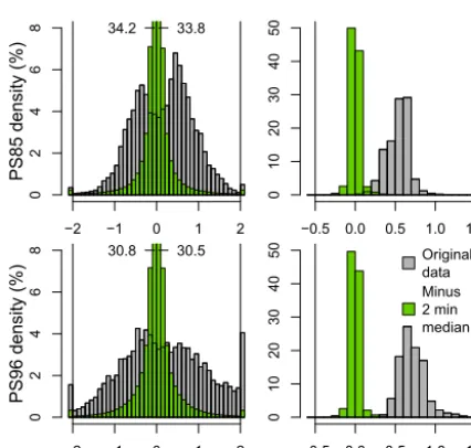
Figure 3.Frequency distribution of the ship angle (grey) and ship angle minus a 2 min running median (green) during the measure-ment time.
A variety of different scanning programs were used: ver-tical azimuth display (VAD), horizontal stare in two or three directions, range-height indicator (RHI) and vertical stare. In the present paper we will focus on the VAD measurements that allow the computation of vertical profiles of horizontal wind speed. One VAD scan is composed of eight rays with fixed elevation and different azimuth (0, 45, 90, 135, 180, 225, 270, 315◦). During PS96 we changed the elevation from 85 to 75◦after 3 days. The averaging time for each ray was usually 12–15 s. During PS85 the averaging time for each ray was only 1.5 s but azimuth circles were done at 25, 50 and 75◦ elevation. For the analysis we will either use only the 75◦or all 25, 50 and 75◦elevations. To make them com-parable when using all three elevations, we will count the 3×8=24 rays as one VAD. One ray is divided into sections of 3 m length and one measured Doppler velocity is repre-sentative for gate length of six sections (18 m). During PS85 those six sections were non-overlapping; thus measurements were available every 18 m. During PS96 the six sections were
overlapping; thus measurements were available every 3 m. But the measurements with overlapping sections are not in-dependent as they are computed based partially on same data. VAD wind profiles are typically available every 15 min and a whole VAD scan required about 2 min for PS96. Photos of the weather condition were taken manually for special sit-uations during PS85 and automatically with a GoPro (with constant power connection) every minute during PS96. 2.2 Radiosondes
Radiosondes at Polarstern (König-Langlo, 2014a, 2016a) were usually launched twice a day at 05:00 and 11:00 UTC during PS85 (39 radiosondes over the 18 days) and 07:00 and 11:00 UTC during PS96 (70 radiosondes over the 38 days). Radiosondes of the type Vaisala RS92 (Vaisala, 2013) were used. The measurement uncertainty for wind is specified as 0.15 m s−1for speed and 2◦for direction. For the intercom-parison of lidar wind profiles with the radiosonde profiles additional aspects to instrumental errors have to be consid-ered. As shown below, the vertical range of the lidar is gen-erally limited to the height of the ABL of a few hundred me-tres. When the ship is cruising, the radiosondes are launched close to the ship’s superstructure and are affected by the tur-bulent wake of the ship. The radiosonde also needs time to accelerate to the ambient wind speed after launch, and ex-hibits strong pendulum motions during this phase. This re-sults in a strong noise in the raw wind data, and a low-pass filter is applied, resulting in a reduced vertical resolution (es-timated as about 200 m by Päschke et al., 2015). As docu-mented by Achert et al. (2015) for the RVOden, the ship’s superstructure modifies the mean flow depending on flow di-rection. The largest effect occurs for relative wind along the ship’s axis. For these conditions, the disturbance decreases with height and is estimated as smaller than 2 % for horizon-tal wind speeds at altitudes above 75 m. For a flow that is perpendicular to the ship, this effect also reduces to 2 % be-low 75 m. A study of Berry et al. (2001) for RVPolarstern
2.3 Analysis of the lidar data
The wind analysis consists of different steps. First we look at the influence and correction of the ship’s motions. In the sec-ond part we describe our data processing method and com-putation of horizontal winds. In the third part we discuss our choice of the SNR threshold.
2.3.1 Ship’s motion correction
The main difficulty in receiving reliable wind data results from the movements of the ship. The ship’s velocity and ori-entation and their changes influence the directions of the li-dar’s outgoing and incoming rays. Therefore the ship’s ve-locity and orientation angles are the two main factors for the correction of the measured data. During both cruises PS86 and PS96, the ship was moving with more than 1 m s−1about
50 % of the time. The lidar was aligned with the ship by eye as best as possible (deviations of the yaw angle between li-dar and the ship are discussed later in the results section). Measured ship data from the scientific navigational platform are taken to correct each single lidar measurement by the ship’s speed and roll–pitch–yaw angles. The resolution of these data is 1 Hz. The correction for the ship’s roll and pitch movements can be avoided by using a motion-stabilizing platform (Achtert et al., 2015). We had no such platform, but additionally to the ship’s 1 Hz navigation data, we also recorded roll and pitch movements at high-frequency (up to 400 Hz) by the AHRS that was attached to the lidar. The AHRS data were used to determine the roll and pitch off-set between the AHRS (or lidar) reference system and the ships reference system. During PS96 the averaging time of a single ray was typically 12–15 s, so that we corrected each single measurement with the mean value over the averaging time. This introduces an error whenever the ship angle, and thus the lidar angle, changes during this averaging time. In order to reduce the error, all measurements that have a stan-dard deviation of roll or pitch angle larger than 0.5◦or yaw angle larger than 2◦over this averaging time were excluded from the analysis. Correcting the direction of the lidar mea-surement by the mean roll and pitch angle during the aver-aging time should already cause most of the error to average out, as it measures partly too much and partly too little wind speed. But even if this is not the case, for a data point at 1 km distance from the lidar a change in elevation from 75 to 75.5◦(25 to 25.5◦) causes a difference in height of 2 m (8 m) and the resulting horizontal wind speed error is less than 3.3 % (0.4 %). This is acceptable as we will later in-terpolate over height intervals of 50 m and only evaluate the horizontal wind in our paper. It should be noted that the cor-rection and filtering process causes almost no loss of data. Only 6 % of the time is the standard deviation of the yaw angle over 15 s larger than 2◦and the ship’s movement even during ice breaking conditions generally does not result in high-frequency changes of roll and pitch (except some cases
of ramming). The important part is in fact the low-frequency change in roll and pitch (e.g. pumping water from one tank to another, changing cargo) that gets corrected. This can be seen by subtracting a 2 min running median from the roll and pitch data (Fig. 3). The remaining angles are within−0.1 and 0.1◦60–70 % of the time. Without roll and pitch correction, values amount from−2 to 2◦for roll (for 95 % of the cases) and 0 to 1.5◦for pitch. Therefore a set-up without any roll or pitch correction at all would still provide usable data if a high data quality is not of importance. For example, for a data point at a 1 km distance from the lidar a change in elevation from 75 to 77◦ (25 to 27◦) causes a difference in height of 8 m (31 m) and horizontal wind speed error of less than 13 % (17 %). We also corrected for the influence of the angular velocity of roll pitch and yaw, but it was found to be negligible. For PS96 (PS85) the correction due to angular velocity was less than 0.2 m s−199.7 % (99.9 %) of the time
and never greater than 0.5 m s−1.
2.3.2 Data processing
First, an SNR threshold was chosen and all data points within one ray with a worse SNR were removed. The SNR is a value given in the lidar output for each scanned Doppler veloc-ity value. It is separate from the empirical noise defined in Sect. 2.3.3 as well as from the “noisy influence” due to other error sources like uncertainties related to the ships move-ment. The background noise is usually measured at least once a day and at most every hour. For this, the scanning head is turned away from the sky towards the lidar casing and mea-sures the signal while sending no pulses out. Thus the back-ground noise can vary with time and operating conditions and can be different for different HALO instruments. To com-pute the SNR, the signal strength of the background noise is subtracted from the signal strength of the measurement and afterwards divided by the signal strength of the background noise. If the signal during a measurement is lower than dur-ing the background noise scan, it can therefore cause a neg-ative SNR. In general, more background noise scans were performed during PS85, but we did not investigate the back-ground noise further.
Furthermore the first data points near the lidar were re-moved (approx. the first 30 m) as these measurements are of-ten affected by the outgoing pulse. Then each single ray was segmented into bins of 100 m. For each bin, outliers (radial velocity>3×standard deviation) were removed. If less than 50 % of the data remained or if the standard deviation of the radial velocity of remaining data in the bin was greater than 3 m s−1, the whole bin was removed.
horizon-0 20 40 60 80 100
(a) PS85 (25°,50°,75°)
0
0
0
500
1000
1500
Height (m)
0 20 40 60 80 100
(b) PS85 (75°)
0
0
Computed horizontal winds (%)
SNR threshold
(dB) −30 −25 −24 −23 −22 −21 −20 −19 −18 −17 −16 −15 SNR threshold
(dB) −30 −25 −24 −23 −22 −21 −20 −19 −18 −17 −16 −15
0 20 40 60 80 100
(c) PS96 (75°)
0
0
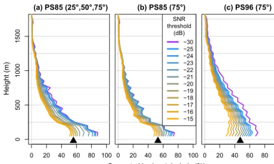
Figure 4.Percentage of wind calculations (speed and direction) from VAD scans as a function of SNR threshold at different heights during PS85 using all elevations(a), only an elevation of 75◦(b)and PS96(c). The total number of VADs for PS85/PS96 was 3552/4250. The black triangle indicates the chosen SNR threshold based on Fig. 5. For the height between 0 and 1750 m this chosen threshold results in 15 % (PS85, all elevations), 14 % (PS85, only 75◦) or 21 % (PS96) of computed horizontal winds.
tally homogenous in each layer. The general approach for the processing of VAD scans is the calculation of the 3-D wind by finding the solution to a system of equations. There are two common perspectives on their definition. The first per-spective operates in the (local) Cartesian coordinate system (east, north, up), in which wind is described by the compo-nents (u,v,w) and the direction of the lidar beam (normal-ized radius vector (xL,yL,zL)). Each measured Doppler
ve-locityd (negative if wind is blowing towards the lidar) satis-fies the following linear equation:
d=xL·u+yL·v+zL·w. (1)
The second perspective describes wind with horizontal wind speed and direction and the vertical component (vh=
√
u2+v2horizontal wind speed,φ
hwind direction,w). The
Doppler velocity is then a function of the scanning directions in polar coordinates (φ=azimuth,θ=elevation).
d=cos(φ−φh−π )·vh·cos(θ )+sin(θ )·w (2)
As Eq. (1) can be transformed into Eq. (2), they are equiva-lent (see Appendix). Assuming that the lidar remains station-ary and has a fixed elevation angleθ(which is not the case in our set-up), the equation further simplifies to
d c1
=cos(φ−φh−π )·vh+w·c2, (3)
with the constantsc1=cos(θ )andc2=tan(θ ). Wind speed
and direction can then be determined by a cosine fit for all available scan directions. Although the Eqs. (2) and (3) are more intuitive, and our lidar software already uses the param-eters elevation and azimuth, we found it is easier to work in a Cartesian coordinate system to apply corrections and thus choose Eq. (1). Since we have eight rays per VAD (and more
than one measurement per ray in each layer), we get a system of linear equations. Given a measured set of Doppler veloci-tiesdi (i=1, . . ., n) in directions (xi,yi,zi) (east, north, up),
the wind speed (u,v,w) can be calculated by solving the overdetermined system:
x1 y1 z1 x2 y2 z2 . . . . xn yn zn
×
u v w
=
d1 d2 . . . dn
(4)
using the least squares method. To ensure the quality of the data we added the condition that at least six out of eight az-imuth angles had data (that was not removed); thus at least measurements in a sector of 270◦were available.
As the system of equations is only solved approximately for a given a solution(u∗, v∗, w∗), we can define a measure for the goodness of the fit. Päschke et al. (2015) define the coefficient of determination. We define the fit deviation in our paper as follows:
x1 y1 z1 x2 y2 z2 . . . . xn yn zn
×
u∗ v∗ w∗
−
d1 d2 . . . dn
2
. (5)
For the purpose of comparing the fit deviation, only scans with the same elevation should be used. It should also be noted that measuring a non-homogenous or non-stationary wind field would result in a larger fit deviation value.
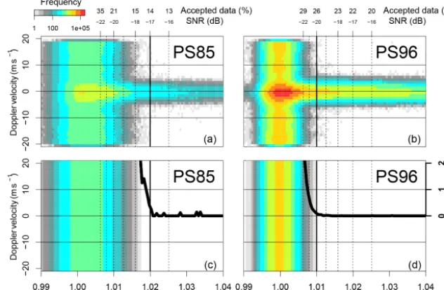
Figure 5. (a, b)Frequency of Doppler velocities of VAD scans with 75◦elevation depending on the intensity/SNR and for PS85(a, c)and PS96(b, d). Bottom row: empirical noise computed as the mean for points above 10 m s−1or below−10 m s−1. The solid black line shows the ratio of empirical noise and all measured data(a, b)at each intensity/SNR. On the top axis it is also noted how much data would be accepted if the respective (minimal) SNR was chosen.
this 100 m bin combined with computing winds every 50 m. It is more dominant for PS96 as the measurement was taken every 3 m, while the measurements for PS85 were taken ev-ery 18 m. The benefit of using additional scans with 25 and 50◦ elevation for PS85 can be seen for the lowest 750 m if a higher SNR threshold is chosen. The choice of the SNR threshold for this paper is explained in the next section. 2.3.3 Choice of signal-to-noise ratio thresholds
SNR-based thresholds for the separation between reliable and unreliable data points are a common technique for lidar data processing (Päschke et al., 2015; Pearson et al., 2009; Frehlich and Yadlowsky, 1994; Barlow et al., 2011). This value can vary depending on the instrument-specific perfor-mance (detector noise) and the variability of atmospheric conditions within the measured volume. The recommenda-tion of the manufacturer for the lidar is −18.2 dB. How-ever, Päschke et al. (2015) showed that this value is rather conservative and reduces the amount of data by up to 40 % (between −20 and−18.2 dB). Hirsikko et al. (2014) use a threshold of −21 dB and state that−25 dB could still suit-able for horizontal wind measurements. Pearson et al. (2009) experimentally find an SNR threshold for reliable data of
−23 dB. The potential SNR threshold was already consid-ered during our measurements by adjusting the telescope fo-cal length of the lidar and the integration time (following the recommendations Hirsikko et al., 2014). This is necessary during the measurements, since raw data on single pulses were not stored and thus no post-processing is possible. Fig-ure 4 shows the sensitivity of available data for PS85 and
0
0 60
0
500
1000
1500
Height (m)
(a) PS85 N SNR threshold
(dB) −23 −20 −17 SNR threshold
(dB) −23 −20 −17
0
0 1 2
Wind speed (m s−1) RMSD
0
−1 1 bias
0
0 20
Wind direction (°) RMSD
0
−10 10 bias
0
0 60
(b) PS96 N
0
0 1 2
Wind speed (m s−1) RMSD
0
−1 1 bias
0
0 20
Wind direction (°) RMSD
0
−10 10 bias
Figure 6.RMSD, bias and number of used radio soundings (N) by height of wind speed and direction for PS85(a)and PS96(b). Different colours show different SNR thresholds (−23 blue,−20 dB green,−17 dB orange). Only scans with an elevation of 75◦were used.
Table 2.Statistics for all available lidar data compared to radio soundings.Mindicates the number of used radio soundings.Nindicates the number of compared measurements (Nis lower for the wind direction because up to six cases with wind speed<0.5 m s−1are removed). PS85 computed for a−17 dB SNR threshold with only 75◦elevation scans (first column, as shown in Fig. 6) and with all 25, 50 and 75◦ (second column). PS96 was computed for−20 dB SNR threshold with the default case (standard deviation of yaw angle below 2◦for each ray; third column, as shown in Fig. 6) and a stricter case (standard deviation of yaw angle below 0.5◦for each ray; fourth column).aRis the correlation coefficient for angular variables.
Wind speed in m s−1 Wind direction in degrees
M N RMSD Bias R2 RMSD Bias aR2
PS85 (VAD with 75◦) 28 216 0.7 0.1 0.95 6 2 0.99
PS85 (25, 50, 75◦) 28 226 0.7 −0.1 0.95 6 −3 0.99
PS96 (2◦yaw-sd) 58 574 0.8 0.1 0.95 11 0 0.96
PS96 (0.5◦yaw-sd) 49 502 0.8 0.0 0.96 12 0 0.95
signal (relatively homogenous along the signal intensity or SNR; left to right). Signal intensity is defined as SNR+1. All points above 10 m s−1or below−10 m s−1are taken to construct an empirical noise distribution as a function of in-tensity using the mean value (Fig. 5, bottom). In the second step, we take the ratio of the empirical noise and the mean of the measured Doppler velocities for each intensity, which results in an empirical noise fraction (plotted as solid line in Fig. 5, bottom). The empirical noise fraction is close to zero for high intensities and starts to increase rapidly at different SNR values for both data sets. We choose an SNR thresh-old (step three) of −17 dB for PS85 and −20 dB for PS96. This empirical SNR threshold results in about 14 %/26 % of usable raw data for PS85/96. Comparing this to the result-ing VAD percentages 14 %/21 % (Fig. 4), it should be noted that the decrease for PS96 comes mostly from the restriction sd(yaw) <2◦ and sd(roll/pitch)<0.5◦. Without this condi-tion, the computed VAD percentage is 25 %.
3 Results
dif-Table 3. Statistics as in Table 2 but showing the range of the statistic variables for different computations. These include all possible combinations of the following two (default marked with∗): (1) the thickness of layers and thus the interpolation in height of lidar data [10, 20, 30, 40, 50∗m] and (2) the time range of used lidar measurements around the radio sounding measurement (100 s after start) [±5, 10∗, 15, 30 min].
Wind speed in m s−1 Wind direction in degrees
M N RMSD Bias R2 RMSD Bias aR2
PS85 (VAD with 75◦) 27–28 192–489 0.7 0.1–0.1 0.95–0.96 5–6 1–2 0.99
PS85 (25, 50, 75◦) 28 207–508 0.6–0.7 −0.1–0.0 0.95–0.96 6 −3 0.99
PS96 (2◦yaw-sd) 39–60 369–1391 0.7–0.8 0.0–0.1 0.95–0.96 11–14 0–1 0.96–0.97 PS96 (0.5◦yaw-sd) 32–51 316–1226 0.7–0.8 0.0–0.1 0.96–0.97 12–15 0–1 0.95–0.97
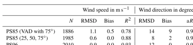
Table 4.Statistics for lidar data (at approx. 50–75 m) compared to the ship anemometer (at 39 m).Nindicates the number of comparisons (for the wind direction, one case with wind speed<0.5 m s−1was removed).aRis the correlation coefficient for angular variables.
Wind speed in m s−1 Wind direction in degrees
N RMSD Bias R2 RMSD Bias aR2
PS85 (VAD with 75◦) 1886 1.1 0.5 0.78 14 9 0.96
PS85 (25, 50, 75◦) 1985 0.6 0.0 0.88 8 2 0.98
PS96 2010 0.9 0.0 0.93 12 0 0.95
ferences, particularly for PS85, our empirical thresholds of
−20 and−17 dB are found to be reasonable. Furthermore, a systematic dependence on height is not present. We also check for a height dependence of the correlation (not shown), but there was none present. At heights above 1000 m the sam-ple size is relatively small and differences between different SNR thresholds are not robust.
The overall statistics of the radiosonde comparisons are shown in Table 2. Although our data set is smaller than that of Achtert et al. (2015), we find similar results (RMSD for wind speed around 1 m s−1and wind direction around 10◦). The biases for the wind speed and direction are very small. When applying a stricter condition for the allowed standard deviation of yaw angle during the measuring and averaging time (last row in Table 2), a clear improvement in the data quality is not seen.
In order to quantify the impact of changes in our stan-dard data processing, the effects of changing the layer thick-ness and changing the averaging time around the radiosonde launch were investigated. Table 3 summarizes the ranges of the effects RMSD, bias andR2. None of these changes had any relevant influence. We also computed the 95 % confi-dence interval bounds for the biases and found them to be 0.1 m s−1and 1◦higher or lower than the biases given in Ta-bles 2 and 3.
As mentioned above, our results are similar to Achert et al. (2015), who used a motion-stabilized platform and found mean bias for wind speed and direction of 0.3 m s−1and 2◦, and a mean standard deviation of 1.1 m s−1and 12◦for wind speed and direction respectively. Since the lidar was aligned with the ship’s axis only by eye (see Sect. 2), this might
cause a yaw offset. We tried to estimate this yaw offset by checking the correlation of the roll and pitch 1 Hz data from the AHRS (or lidar) and the ship’s navigation system. By assuming a yaw offset and correcting the roll and pitch an-gles, we determined the peak of the correlation. As a result, we found lidar yaw offsets of around−0.5◦ for PS85 and
+1◦for PS96 which are in the range of the observed bias. It should be mentioned that the first evaluations yielded a bias of 5 to 7◦in wind direction compared to the radio soundings. During maintenance of the lidar after the cruises a misalign-ment of the lidar scanning direction by the manufacturer was discovered (offset of 5.32◦in azimuth). This correction was applied to the present evaluations.
In a second analysis we compared the winds measured on the crow’s nest of the ship (König-Langlo, 2014b, 2016b). There are two anemometers (2-D-sonic anemometers, one at each side, König-Langlo et al., 2006) mounted at a height of around 39 m above sea level. The first usable data points of the lidar measurements are at approximately 50 m height. Comparing the wind direction measured by the lidar in 50 m with wind direction in 60 to 200 m, we found an overall lin-ear increase (decrease) of wind direction with height during PS85 (PS96). Assuming this change in wind direction is also present between the 39 m anemometer and the lidar data (ap-prox. 50–75 m), this could lead to a slight positive (negative) bias during PS85 (PS96) of about 1◦. An overview is shown in Figs. 7 and 8 and the statistics computed for this compari-son are shown in Table 4.