Natural
Resources
Biometrics
Dr. Diane Kiernan
SUNY
College of Environmental
Natural Resources Biometrics
Dr. Diane Kiernan
Open SUNY Textbooks
2014 Diane Kiernan
This work is licensed under a
Creative Commons Attribution-NonCommercial-ShareAlike 3.0 Unported License.
Published by Open SUNY Textbooks, Milne Library (IITG PI)
State University of New York at Geneseo,
About this Textbook
Natural Resources Biometrics begins with a review of descriptive statistics, estimation, and hypothesis testing. The following chapters cover one- and two-way analysis of variance (ANOVA), including multiple comparison methods and interaction assessment, with a strong emphasis on application and interpretation. Simple and multiple linear regressions in a natural resource setting are covered in the next chapters, focusing on correlation, model fitting, residual analysis, and confidence and prediction intervals. The final chapters cover growth and yield models, volume and biomass equations, site index curves, competition indices, importance values, and measures of species diversity, association, and community similarity.
About the Author
Diane Kiernan, Ph.D., Instructor at the SUNY College of Environmental
Science and Forestry
Reviewer’s Notes
Dr. Diane H. Kiernan is an expert on forest biometrics and growth and yield modeling, and is an experienced writer for textbooks of applied statistics. She has been teaching the course Introductory Statistics to sophomore students at SUNY-ESF over the last five years, and has been recently assigned to teach the biometrics / applied statistics course at a junior / senior level to a wide range of majors in the college.
The purposes of this textbook are (1) to review basic concepts and methods that the students have learned in the Introductory Statistics course such as descriptive statistics, confidence intervals, and one-sample and two-samples hypothesis testing, (2) to teach the funda-mental concepts, principles, and methods of Analysis of Variance (ANOVA) and simple and multiple linear regression analysis, (3) to introduce students to statistical software such as Minitab and Microsoft Excel for data analysis and statistical computing with real world examples, and (4) to cover some topics related to forest and natural resources management, such as site index curves, stand density management diagrams, stocking charts, volume tables, forest growth and yield models, species diversity, etc.
Given her extensive teaching experience, Dr. Kiernan presents the fundamental concepts, principles, and methods of statistics in “layman” English, without mathematical proofs on the theories. Instead she provides clear and logical explanation and demonstration on how to apply these statistical theories and methods to solve the problems and answer the ques-tions that the students may encounter in their studies and practices. The examples used in the textbook are closely related to forestry, biology, water, wildlife, environment, as well as social sciences. The textbook is most suitable to a one-semester course for the curriculums of forest and natural resources management, forest biology, forest ecosystem sciences.
Dr. Lianjun Zhang, Ph.D.
About Open SUNY Textbooks
Open SUNY Textbooks is an open access textbook publishing initiative established by State University of New York libraries and supported by SUNY Innovative Instruction Technology Grants. This initiative publishes high-quality, cost-effective course resources by engaging faculty as authors and peer-reviewers, and libraries as publishing infrastructure.
The pilot launched in 2012, providing an editorial framework and service to authors, stu-dents and faculty, and establishing a community of practice among libraries. The first pilot is publishing 15 titles in 2013-2014, with a second pilot to follow that will add more textbooks and participating libraries.
Participating libraries in the 2012-2013 pilot include SUNY Geneseo, College at Brock-port, College of Environmental Science and Forestry, SUNY Fredonia, Upstate Medical University, and University at Buffalo, with support from other SUNY libraries and SUNY Press.
Contents
Chapter 1
Descriptive Statistics and the Normal Distribution
1
Chapter 2
Sampling Distributions and Confidence Intervals
28
Chapter 3
Hypothesis Testing
43
Chapter 4
Inferences about the Differences of Two Populations
81
Chapter 5
One-Way Analysis of Variance
117
Chapter 6
Two-way Analysis of Variance
131
Chapter 7
Correlation and Simple Linear Regression
150
Chapter 8
Multiple Linear Regression
182
Chapter 9
Modeling Growth, Yield, and Site Index
199
Chapter 10
Quantitative Measures of Diversity, Site Similarity, and Habitat
Suitability
216
Appendix
Biometrics Lab #1
228
Biometrics Lab #2
233
Biometrics Lab #3
238
Chapter 1
Descriptive Statistics and the
Normal Distribution
Statistics has become the universal language of the sciences, and data analysis can lead to powerful results. As scientists, researchers, and managers working in the natural resources sector, we all rely on statistical analysis to help us answer the questions that arise in the populations we manage. For example:
• Has there been a significant change in the mean sawtimber volume in the red pine stands?
• Has there been an increase in the number of invasive species found in the Great Lakes?
• What proportion of white tail deer in New Hampshire have weights below the limit considered healthy?
• Did fertilizer A, B, or C have an effect on the corn yield?
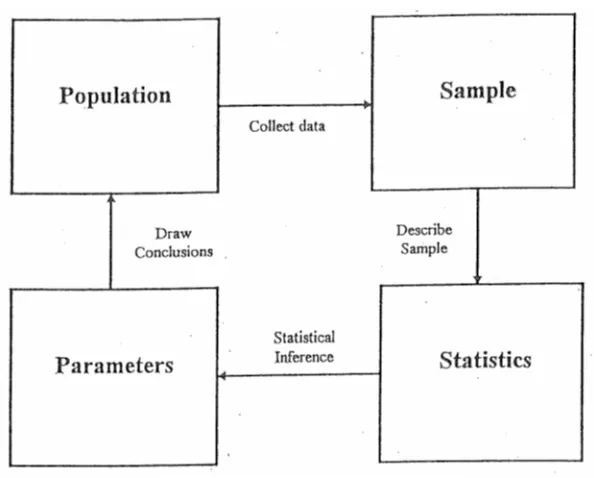
These are typical questions that require statistical analysis for the answers. In order to answer these questions, a good random sample must be collected from the population of interests. We then use descriptive statistics to organize and summarize our sample data. The next step is inferential statistics, which allows us to use our sample statistics and extend the results to the population, while measuring the reliability of the result. But before we begin exploring different types of statistical methods, a brief review of descriptive statistics is needed.
Statistics is the science of collecting, organizing, summarizing, analyzing, and interpreting information.
Figure 1. Using sample statistics to estimate population parameters.
Section 1
Descriptive Statistics
A population is the group to be studied, and population data is a collection of all elements in the population. For example:
• All the fish in Long Lake.
• All the lakes in the Adirondack Park.
• All the grizzly bears in Yellowstone National Park.
A sample is a subset of data drawn from the population of interest. For example:
• 100 fish randomly sampled from Long Lake.
• 25 lakes randomly selected from the Adirondack Park.
• 60 grizzly bears with a home range in Yellowstone National Park.
esti-3
Natural Resources Biometrics Chapter 1
mated by the sample mean (x). The population variance (σ2) is estimated by the sample
variance (s2).
Variables are the characteristics we are interested in. For example:
• The length of fish in Long Lake.
• The pH of lakes in the Adirondack Park.
• The weight of grizzly bears in Yellowstone National Park.
Variables are divided into two major groups: qualitative and quantitative. Qualitative variables have values that are attributes or categories. Mathematical operations cannot be applied to qualitative variables. Examples of qualitative variables are gender, race, and petal color. Quantitative variables have values that are typically numeric, such as measurements. Mathematical operations can be applied to these data. Examples of quantitative variables are age, height, and length.
Quantitative variables can be broken down further into two more categories: discrete and continuous variables. Discrete variables have a finite or countable number of possible values. Think of discrete variables as “hens”. Hens can lay 1 egg, or 2 eggs, or 13 eggs… There are a limited, definable number of values that the variable could take on.
Continuous variables have an infinite number of possible values. Think of continuous variables as “cows”. Cows can give 4.6713245 gallons of milk, or 7.0918754 gallons of milk, or 13.272698 gallons of milk … There are an almost infinite number of values that a continuous variable could take on.
Ex. 1
Is the variable qualitative or quantitative?
Species Weight Diameter Zip Code
Descriptive Measures
Descriptive measures of populations are called parameters and are typically written using Greek letters. The population mean is μ (mu). The population variance is σ2 (sigma squared)
and population standard deviation is σ (sigma).
Descriptive measures of samples are called statistics and are typically written using Roman letters. The sample mean is x(x-bar). The sample variance is s2 and the sample standard
deviation is s. Sample statistics are used to estimate unknown population parameters.
In this section, we will examine descriptive statistics in terms of measures of center and measures of dispersion. These descriptive statistics help us to identify the center and spread of the data.
Measures of Center
Mean
The arithmetic mean of a variable, often called the average, is computed by adding up all the values and dividing by the total number of values.
The population mean is represented by the Greek letter μ (mu). The sample mean is represented by
x
(x-bar). The sample mean is usually the best, unbiased estimate of the population mean. However, the mean is influenced by extreme values (outliers) and may not be the best measure of center with strongly skewed data. The following equations com-pute the population mean and sample mean.µ
=
∑
x
N
i
x
x
n
i
=
∑
where xi is an element in the data set, N is the number of elements in the population, and
n is the number of elements in the sample data set.
Ex. 2
Find the mean for the following sample data set: 6.4, 5.2, 7.9, 3.4
x
=
6 4
+
5 2
+
7 9
+
3 4
=
4
5 725
.
.
.
.
5
Natural Resources Biometrics Chapter 1
Median
The median of a variable is the middle value of the data set when the data are sorted in order from least to greatest. It splits the data into two equal halves with 50% of the data below the median and 50% above the median. The median is resistant to the influence of outliers, and may be a better measure of center with strongly skewed data.
The calculation of the median depends on the number of observations in the data set.
To calculate the median with an odd number of values (n is odd), first sort the data from smallest to largest.
Ex. 3
23, 27, 29, 31, 35, 39, 40, 42, 44, 47, 51
The median is 39. It is the middle value that separates the lower 50% of the data from the upper 50% of the data.
To calculate the median with an even number of values (n is even), first sort the data from smallest to largest and take the average of the two middle values.
Ex. 4
23, 27, 29, 31, 35, 39, 40, 42, 44, 47
M
=
35
+
39
=
2
37
Mode
Understanding the relationship between the mean and median is important. It gives us insight into the distribution of the variable. For example, if the distribution is skewed right (positively skewed), the mean will increase to account for the few larger observations that pull the distribution to the right. The median will be less affected by these extreme large values, so in this situation, the mean will be larger than the median. In a symmetric distri-bution, the mean, median, and mode will all be similar in value. If the distribution is skewed left (negatively skewed), the mean will decrease to account for the few smaller observations that pull the distribution to the left. Again, the median will be less affected by these extreme small observations, and in this situation, the mean will be less than the median.
Figure 2. Illustration of skewed and symmetric distributions.
Measures of Dispersion
Measures of center look at the average or middle values of a data set. Measures of disper-sion look at the spread or variation of the data. Variation refers to the amount that the values vary among themselves. Values in a data set that are relatively close to each other have lower measures of variation. Values that are spread farther apart have higher measures of variation.
Examine the two histograms below. Both groups have the same mean weight, but the values of Group A are more spread out compared to the values in Group B. Both groups have an average weight of 267 lb. but the weights of Group A are more variable.
520 420 320 220 120 20 35 30 25 20 15 10 5 0 Weight A Fr eq ue nc y
Histogram of Group A
350 325 300 275 250 225 200 30 25 20 15 10 5 0 Weight B Fr eq ue nc y
Histogram of Group B
7
Natural Resources Biometrics Chapter 1
This section will examine five measures of dispersion: range, variance, standard deviation, standard error, and coefficient of variation.
Range
The range of a variable is the largest value minus the smallest value. It is the simplest measure and uses only these two values in a quantitative data set.
Ex. 5
Find the range for the given data set. 12, 29, 32, 34, 38, 49, 57
Range = 57 – 12 = 45
Variance
The variance uses the difference between each value and its arithmetic mean. The differ-ences are squared to deal with positive and negative differdiffer-ences. The sample variance (s2) is
an unbiased estimator of the population variance (σ2), with n-1 degrees of freedom.
Degrees of freedom: In general, the degrees of freedom for an estimate is equal
to the number of values minus the number of parameters estimated en route to the estimate in question.
The sample variance is unbiased due to the difference in the denominator. If we used “n” in the denominator instead of “n-1”, we would consistently underestimate the true population variance. To correct this bias, the denominator is modified to “n-1”.
Population variance Sample variance
σ2 =
∑
(
x
−
)
N
i
µ
2
s2 =
∑
∑
∑
− − = −(
)
−(x x)
n x x n n i i i 2 2 2 1 1
Ex. 6
Compute the variance of the sample data: 3, 5, 7. The sample mean is 5.
s
22 2 2
3
5
5
5
7
5
3
1
4
=
−
+ −
+ −
−
=
Standard Deviation
The standard deviation is the square root of the variance (both population and sample). While the sample variance is the positive, unbiased estimator for the population variance, the units for the variance are squared. The standard deviation is a common method for numerically describing the distribution of a variable. The population standard deviation is σ (sigma) and sample standard deviation is s.
Population standard deviation Sample standard deviation
σ
=
σ
2s
=
s
2Ex. 7
Compute the standard deviation of the sample data: 3, 5, 7 with a sample mean of 5.
s
=
−
+ −
+ −
−
=
=
(
3
5
)
(
5
5
)
(
7
5
)
3
1
4
2
2 2 2
Standard Error of the Means
Commonly, we use the sample mean
x
to estimate the population mean μ. For example, if we want to estimate the heights of eighty-year-old cherry trees, we can proceed as follows:• Randomly select 100 trees
• Compute the sample mean of the 100 heights
• Use that as our estimate
We want to use this sample mean to estimate the true but unknown population mean. But our sample of 100 trees is just one of many possible samples (of the same size) that could have been randomly selected. Imagine if we take a series of different random samples from the same population and all the same size:
• Sample 1—we compute sample mean
x
1.• Sample 2—we compute sample mean
x
2.• Sample 3—we compute sample mean
x
3.• Etc.
9
Natural Resources Biometrics Chapter 1
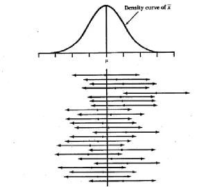
The sample mean (
x
) is a random variable with its own probability distribution called the sampling distribution of the sample mean. The distribution of the sample mean will have a mean equal to µ and a standard deviation equal to s n.The standard error s n is the standard deviation of all possible sample means.
In reality, we would only take one sample, but we need to understand and quantify the sample to sample variability that occurs in the sampling process.
The standard error is the standard deviation of the sample means and can be expressed in different ways.
Note: s2 is the sample variance and s is the sample standard deviation
Ex. 8
Describe the distribution of the sample mean.
A population of fish has weights that are normally distributed with µ = 8 lb. and s = 2.6 lb. If you take a sample of size n=6, the sample mean will have a normal distribu-tion with a mean of 8 and a standard deviadistribu-tion (standard error) of 2 6
6 .
= 1.061 lb. If you increase the sample size to 10, the sample mean will be normally distributed with a mean of 8 lb. and a standard deviation (standard error) of 2 6
10 .
= 0.822 lb. Notice how the standard error decreases as the sample size increases.
The Central Limit Theorem (CLT) states that the sampling distribution of the sample means will approach a normal distribution as the sample size increases. If we do not have a normal distribution, or know nothing about our distribution of our random variable, the CLT tells us that the distribution of the
x
’s will become normal as n increases. How large does n have to be? A general rule of thumb tells us that n ≥ 30.The Central Limit Theorem tells us that regardless of the shape of our population, the sampling distribution of the sample mean will be normal as the sample size
Coefficient of Variation
To compare standard deviations between different populations or samples is difficult because the standard deviation depends on units of measure. The coefficient of variation expresses the standard deviation as a percentage of the sample or population mean. It is a unitless measure.
Population data Sample data
CV =
σ
µ
*100
CV =s
x
*100
Ex. 9
Fisheries biologists were studying the length and weight of Pacific salmon. They took a random sample and computed the mean and standard deviation for length and weight (given below). While the standard deviations are similar, the differences in units between lengths and weights make it difficult to compare the variability. Com-puting the coefficient of variation for each variable allows the biologists to determine which variable has the greater standard deviation.
Sample mean Sample standard deviation
Length 63 cm 19.97 cm
Weight 37.6 kg 19.39 kg
CV
L=
=
19 97
63 0
100
31 7
.
.
*
. %
.
CV
W=
=
19 39
37 6
100
51 6
.
.
*
. %
There is greater variability in Pacific salmon weight compared to length.
Variability
Variability is described in many different ways. Standard deviation measures point to point variability within a sample, i.e., variation among individual sampling units. Coefficient of variation also measures point to point variability but on a relative basis (relative to the mean), and is not influenced by measurement units. Standard error measures the sample to sample variability, i.e. variation among repeated samples in the sampling process. Typi-cally, we only have one sample and standard error allows us to quantify the uncertainty in our sampling process.
Basic Statistics Example using Excel and Minitab
Software
11
Natural Resources Biometrics Chapter 1
ID
X
iX
i2(
X
i−
X
)
(
X
i−
X
)
2 Order1 25 625 -7.27 52.8529 4
2 35 1225 2.73 7.4529 6
3 55 3025 22.73 516.6529 10
4 15 225 -17.25 298.2529 2
5 40 1600 7.73 59.7529 8
6 25 625 -7.27 52.8529 5
7 55 3025 22.73 516.6529 11
8 35 1225 2.73 7.4529 7
9 45 2025 12.73 162.0529 9
10 5 25 -27.27 743.6529 1
11 20 400 -12.27 150.1819 3
Sum 355 14025 0.0 2568.1519
∑
= n1 i i
X
∑
= n
1 i
2 i
X
∑
(
)
=
−
n1 i i
X
X
∑
(
)
=
−
n1 i
2 i
X
X
(1) Sample mean:
X
X
n
i i n=
∑
=1=
355
11
32 27
.
(2) Median = 35
(3) Variance:
S
X
X
n
X
X
i i n i i n i i n 2 2 1 2 1 11
2568 1519
11 1
256 82
=
−
(
)
−
=
−
=
=
−
= = =∑
∑
∑
.
.
−
=
−
( )
−
=
2 21
14025
355
11
11 1
256 82
n
n
.
(4) Standard deviation:
S
=
S
2=
=
256 82
.
16 0256
.
(5) Range: 55 – 5 = 50
(6) Coefficient of variation:
CV
S
X
=
⋅
100
=
16 0256
⋅
=
32 27
100
49 66
.
.
.
%
(7) Standard error of the mean:
S
S
n
S
n
X
=
=
=
13
Natural Resources Biometrics Chapter 1
Software Solutions
Minitab
Open Minitab and enter data in the spreadsheet. Select STAT>Descriptive stats and check all statistics required.
Descriptive Statistics: Data
Variable N N* Mean SE Mean StDev Variance CoefVar Minimum Q1
Data 11 0 32.27 4.83 16.03 256.82 49.66 5.00 20.00
Variable Median Q3 Maximum IQR
Excel
15
Natural Resources Biometrics Chapter 1
Data
Mean
32.27273
Standard Error
4.831884
Median
35
Mode
25
Standard
Deviation
16.02555
Sample Variance 256.8182
Kurtosis
-0.73643
Skewness
-0.05982
Range
50
Minimum
5
Maximum
55
Sum
355
Count
11
Graphical Representation
Data organization and summarization can be done graphically, as well as numerically. Tables and graphs allow for a quick overview of the information collected and support the presentation of the data used in the project. While there are a multitude of available graphics, this chapter will focus on a specific few commonly used tools.
Pie Charts
bass carp catfish perch trout Category
Pie Chart of Fish
Michele Ozz Patty Paul Pete Ralph Smokey Tozia Vanessa Berta Bill Christopher Clyde Fannie Fran Francis Gary Ichabod Category
Pie Chart of Names
Figure 4. Comparison of pie charts.
Bar Charts and Histograms
Bar charts graphically describe the distribution of a qualitative variable (fish type) while histograms describe the distribution of a quantitative variable discrete or continuous vari-ables (bear weight).
trout perch catfish carp bass 20 15 10 5 0 fish Co un t 480 360 240 120 0 14 12 10 8 6 4 2 0 bear weight Fr eq ue nc y
Figure 5. Comparison of a bar chart for qualitative data and a histogram for quantitative data.
17
Natural Resources Biometrics Chapter 1
Boxplots
Boxplots use the 5-number summary (minimum and maximum values with the three quartiles) to illustrate the center, spread, and distribution of your data. When paired with histograms, they give an excellent description, both numerically and graphically, of the data.
With symmetric data, the distribution is bell-shaped and somewhat symmetric. In the boxplot, we see that Q1 and Q3 are approximately equidistant from the median, as are the minimum and maximum values. Also, both whiskers (lines extending from the boxes) are approximately equal in length.
Figure 6. A histogram and boxplot of a normal distribution.
With skewed left distributions, we see that the histogram looks “pulled” to the left. In the boxplot, Q1 is farther away from the median as are the minimum values, and the left whisker is longer than the right whisker.
Figure 7. A histogram and boxplot of a skewed left distribution.
Figure 8. A histogram and boxplot of a skewed right distribution.
Section 2
Probability Distribution
Once we have organized and summarized your sample data, the next step is to identify the underlying distribution of our random variable. Computing probabilities for continuous random variables are complicated by the fact that there are an infinite number of possible values that our random variable can take on, so the probability of observing a particular value for a random variable is zero. Therefore, to find the probabilities associated with a continuous random variable, we use a probability density function (PDF).
A PDF is an equation used to find probabilities for continuous random variables. The PDF must satisfy the following two rules:
1) The area under the curve must equal one (over all possible values of the random variable).
2) The probabilities must be equal to or greater than zero for all possible values of the random variable.
The area under the curve of the probability density function over some interval represents the probability of observing those values of the random variable
19
Natural Resources Biometrics Chapter 1
The Normal Distribution
Many continuous random variables have a bell-shaped or somewhat symmetric distribu-tion. This is a normal distribudistribu-tion. In other words, the probability distribution of its relative frequency histogram follows a normal curve. The curve is bell-shaped, symmetric about the mean, and defined by μ and σ (the mean and standard deviation).
Figure 9. A normal distribution.
There are normal curves for every combination of μ and σ. The mean (μ) shifts the curve to the left or right. The standard deviation (σ) alters the spread of the curve. The first pair of curves have different means but the same standard deviation. The second pair of curves share the same mean (μ) but have different standard deviations. The pink curve has a smaller standard deviation. It is narrower and taller, and the probability is spread over a smaller range of values. The blue curve has a larger standard deviation. The curve is flatter and the tails are thicker. The probability is spread over a larger range of values.
Figure 10. A comparison of normal curves.
Properties of the normal curve:
• The mean is the center of this distribution and the highest point.
• The curve is symmetric about the mean. (The area to the left of the mean equals the area to the right of the mean.)
• The total area under the curve is equal to one.
• As x increases and decreases, the curve goes to zero but never touches.
• The PDF of a normal curve is y e
x
=
− −
1
2
2 2
2 π σ
µ σ ( )
.
• A normal curve can be used to estimate probabilities.
• A normal curve can be used to estimate proportions of a population that have certain x-values.
The Standard Normal Distribution
21
Natural Resources Biometrics Chapter 1
Standard Normal Table
• The standard normal table gives probabilities associated with specific Z-scores.
• The table we use is cumulative from the left.
• The negative side is for all Z-scores less than zero (all values less than the mean).
• The positive side is for all Z-scores greater than zero (all values greater than the mean).
• Not all standard normal tables work the same way.
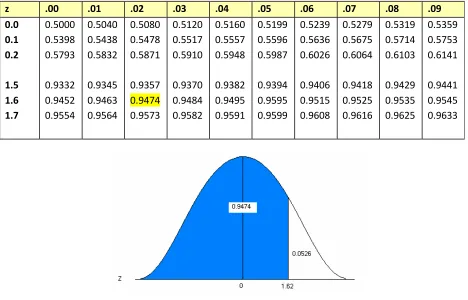
Ex. 10
What is the area associated with the Z-score 1.62?
z .00 .01 .02 .03 .04 .05 .06 .07 .08 .09
0.0 0.5000 0.5040 0.5080 0.5120 0.5160 0.5199 0.5239 0.5279 0.5319 0.5359
0.1 0.5398 0.5438 0.5478 0.5517 0.5557 0.5596 0.5636 0.5675 0.5714 0.5753
0.2 0.5793 0.5832 0.5871 0.5910 0.5948 0.5987 0.6026 0.6064 0.6103 0.6141
1.5 0.9332 0.9345 0.9357 0.9370 0.9382 0.9394 0.9406 0.9418 0.9429 0.9441
1.6 0.9452 0.9463 0.9474 0.9484 0.9495 0.9595 0.9515 0.9525 0.9535 0.9545
1.7 0.9554 0.9564 0.9573 0.9582 0.9591 0.9599 0.9608 0.9616 0.9625 0.9633
Figure 11. The standard normal table and associated area for z = 1.62.
Reading the Standard Normal Table
• Read down the Z-column to get the first part of the Z-score (1.6).
• The intersection of this row and column gives the area under the curve to the left of the Z-score.
Finding Z-scores for a Given Area
• What if we have an area and we want to find the Z-score associated with that area?
• Instead of Z-score → area, we want area → Z-score.
• We can use the standard normal table to find the area in the body of values and read backwards to find the associated Z-score.
• Using the table, search the probabilities to find an area that is closest to the probability you are interested in.
Ex. 11
To find a Z-score for which the area to the right is 5%:
Since the table is cumulative from the left, you must use the complement of 5%. 1.000 – 0.05 = 0.9500
Figure 12. The upper 5% of the area under a normal curve.
• Find the Z-score for the area of 0.9500.
23
Natural Resources Biometrics Chapter 1
Figure 13. The standard normal table.
The Z-score for the 95th percentile is 1.64
Area in between Two Z-scores
Ex. 12
To find Z-scores that limit the middle 95%:
• The middle 95% has 2.5% on the right and 2.5% on the left.
• Use the symmetry of the curve.
Figure 14. The middle 95% of the area under a normal curve.
• Look at your standard normal table. Since the table is cumulative from the left, it is easier to find the area to the left first.
• Find the area of 0.025 on the negative side of the table.
• The Z-score for the area to the left is -1.96.
Common Z-scores
There are many commonly used Z-scores:
• Z.05 = 1.645 and the area between -1.645 and 1.645 is 90%
• Z.025 = 1.96 and the area between -1.96 and 1.96 is 95%
• Z.005 = 2.575 and the area between -2.575 and 2.575 is 99%
Applications of the Normal Distribution
Typically, our normally distributed data do not have μ = 0 and σ = 1, but we can relate any normal distribution to the standard normal distributions using the Z-score. We can transform values of x to values of z.
z x
=
−
µ
σ
For example, if a normally distributed random variable has a μ = 6 and σ = 2, then a value of x = 7 corresponds to a Z-score of 0.5.
Z
=
7
−
6
=
2
0 5
.
This tells you that 7 is one-half a standard deviation above its mean. We can use this rela-tionship to find probabilities for any normal random variable.
Figure 15. A normal and standard normal curve.
25
Natural Resources Biometrics Chapter 1
z x
=
−
µ
σ
Ex. 13
Adult deer population weights are normally distributed with µ = 110 lb. and σ = 29.7 lb. As a biologist you determine that a weight less than 82 lb. is unhealthy and you want to know what proportion of your population is unhealthy.
P(x<82)
Figure 16. The area under a normal curve for P( x<82).
Convert 82 to a Z-score z=82−110= −
29 7
0 94 .
.
The x value of 82 is 0.94 standard deviations below the mean.
Figure 17. Area under a standard normal curve for P(z<-0.94).
Go to the standard normal table (negative side) and find the area associated with a Z-score of -0.94.
This is an “area to the left” problem so you can read directly from the table to get the probability.
P(x<82) = 0.1736
Ex. 14
Statistics from the Midwest Regional Climate Center indicate that Jones City, which has a large wildlife refuge, gets an average of 36.7 in. of rain each year with a standard deviation of 5.1 in. The amount of rain is normally distributed. During what percent of the years does Jones City get more than 40 in. of rain?
P(x > 40)
Figure 18. Area under a normal curve for P( x>40).
z= 40−36 7 =
5 1
0 65 .
.
. P(x>40) = (1-0.7422) = 0.2578
For approximately 25.78% of the years, Jones City will get more than 40 in. of rain.
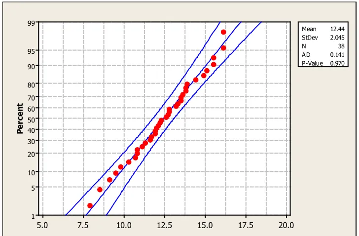
Assessing Normality
If the distribution is unknown and the sample size is not greater than 30 (Central Limit Theorem), we have to assess the assumption of normality. Our primary method is the normal probability plot. This plot graphs the observed data, ranked in ascending order, against the “expected” Z-score of that rank. If the sample data were taken from a normally distributed random variable, then the plot would be approximately linear.
27
Natural Resources Biometrics Chapter 1
20.0 17.5 15.0 12.5 10.0 7.5 5.0 99 95 90 80 70 60 50 40 30 20 10 5 1 Pe rc en t Mean 12.44 StDev 2.045 N 38 AD 0.141 P-Value 0.970
Figure 19. A normal probability plot generated using Minitab 16.
Compare the histogram and the normal probability plot in this next example. The histo-gram indicates a skewed right distribution.
80 70 60 50 40 30 20 10 14 12 10 8 6 4 2 0 Fr eq ue nc y 80 60 40 20 0 -20 99 95 90 80 70 60 50 40 30 20 10 5 1 Pe rc en t Mean 30.17 StDev 16.44 N 31 AD 1.292 P-Value <0.005
Figure 20. Histogram and normal probability plot for skewed right data.
The observed data do not follow a linear pattern and the p-value for the A-D test is less than 0.005 indicating a non-normal population distribution.
Normality cannot be assumed. You must always verify this assumption. Remember, the probabilities we are finding come from the standard NORMAL table. If our data are NOT normally distributed, then these probabilities DO NOT APPLY.
• Do you know if the population is normally distributed?
• Do you have a large enough sample size (n≥30)? Remember the Central Limit Theorem?
Chapter 2
Sampling Distributions and
Confidence Intervals
Sampling Distribution of the Sample Mean
Inferential testing uses the sample mean (
x
) to estimate the population mean (μ). Typically, we use the data from a single sample, but there are many possible samples of the same size that could be drawn from that population. As we saw in the previous chapter, the sample mean (x
) is a random variable with its own distribution.• The distribution of the sample mean will have a mean equal to µ.
• It will have a standard deviation (standard error) equal to σ n.
Because our inferences about the population mean rely on the sample mean, we focus on the distribution of the sample mean. Is it normal? What if our population is not normally distributed or we don’t know anything about the distribution of our population?
The Central Limit Theorem states that the sampling distribution of the sample means will approach a normal distribution as the sample size increases.
• So if we do not have a normal distribution, or know nothing about our distribution, the CLT tells us that the distribution of the sample means (
x
) will become normal distributed as n (sample size) increases.• How large does n have to be?
• A general rule of thumb tells us that n ≥ 30.
29
Natural Resources Biometrics Chapter 2
Sampling Distribution of the Sample Proportion
The population proportion (p) is a parameter that is as commonly estimated as the mean. It is just as important to understand the distribution of the sample proportion, as the mean. With proportions, the element either has the characteristic you are interested in or the element does not have the characteristic. The sample proportion (pˆ) is calculated byp x
n
=
ˆ
where x is the number of elements in your population with the characteristic and n is the sample size.
Ex. 1
You are studying the number of cavity trees in the Monongahela National Forest for wildlife habitat. You have a sample size of n = 950 trees and, of those trees, x = 238 trees with cavities. The sample proportion is:
p
ˆ
=
950
238
=
0 25
.
The distribution of the sample proportion has a mean of
µ
pˆ=
p
and has a standard deviation of
σ
pp
(
p
)
n
=
1
−
ˆ .
The sample proportion is normally distributed if n is very large and
p
ˆ
isn’t close to 0 or 1. We can also use the following relationship to assess normality when the parameter being estimated is p, the population proportion:npˆ
(
1−pˆ)
≥10Confidence Intervals
In the preceding chapter we learned that populations are characterized by descriptive mea-sures called parameters. Inferences about parameters are based on sample statistics. We now want to estimate population parameters and assess the reliability of our estimates based on our knowledge of the sampling distributions of these statistics.
Point Estimates
We start with a point estimate. This is a single value computed from the sample data that is used to estimate the population parameter of interest.
• The sample proportion (
p
ˆ
) is the point estimate of the population proportion (p).We use point estimates to construct confidence intervals for unknown parameters.
• A confidence interval is an interval of values instead of a single point estimate.
• The level of confidence corresponds to the expected proportion of intervals that will contain the parameter if many confidence intervals are constructed of the same sample size from the same population.
• Our uncertainty is about whether our particular confidence interval is one of those that truly contains the true value of the parameter.
Ex. 2
We are 95% confident that our interval contains the population mean bear weight. If we created 100 confidence intervals of the same size from the same population, we would expect 95 of them to contain the true parameter (the population mean weight). We also expect five of the intervals would not contain the parameter.
Figure 1. Confidence intervals from twenty-five different samples.
31
Natural Resources Biometrics Chapter 2
Level of confidence is expressed as a percent.
• The compliment to the level of confidence is α (alpha), the level of significance.
• The level of confidence is described as (1- α) * 100%. What does this really mean?
• We use a point estimate (e.g., sample mean) to estimate the population mean.
• We attach a level of confidence to this interval to describe how certain we are that this interval actually contains the unknown population parameter.
• We want to estimate the population parameter, such as the mean (µ) or proportion (p).
x E
−
< µ <x E
+
orp E
ˆ
−
< p <p E
ˆ
+
where E is the margin of error.
The confidence is based on area under a normal curve. So the assumption of normality must be met (see Chapter 1).
Confidence Intervals about the Mean (
μ
) when the
Population Standard Deviation (
σ
) is Known
A confidence interval takes the form of: point estimate ± margin of error.The point estimate
• The point estimate comes from the sample data.
• To estimate the population mean (μ), use the sample mean (
x
) as the point estimate.The margin of error
• Depends on the level of confidence, the sample size and the population standard deviation.
• It is computed as
E Z
n
=
α∗
σ
2
where
Z
α2is the critical value from the standard normal table associated
with α (the level of significance).
The critical value
Z
α2
• Confidence intervals are ALWAYS two-sided and the Z-scores are the limits of the area associated with the level of confidence.
–
-2
α
Z 2
α
Z
Figure 2. The middle 95% area under a standard normal curve.
• The level of significance (α) is divided into halves because we are looking at the middle 95% of the area under the curve.
• Go to your standard normal table and find the area of 0.025 in the body of values.
• What is the Z-score for that area?
• The Z-scores of ± 1.96 are the critical Z-scores for a 95% confidence interval.
Confidence Level
α (level of significance)
2
α
Z
99%
1%
2.575
95%
5%
1.96
90%
10%
1.645
Table 1. Common critical values (Z-scores).
Construction of a confidence interval about μ when σ is known:
1)
Z
α2 (critical value)
2)
E Z
n
=
α∗
σ
2 (margin of error)
3)
x E
±
(point estimate ± margin of error)Ex. 3
33
Natural Resources Biometrics Chapter 2
Researchers have been studying p-loading in Jones Lake for many years. It is known that mean water clarity (using a Secchi disk) is normally distributed with a popula-tion standard deviapopula-tion of σ = 15.4 in. A random sample of 22 measurements was taken at various points on the lake with a sample mean of
x
= 57.8 in. The researchers want you to construct a 95% confidence interval for μ, the mean water clarity. 1)Z
α2 = 1.96
2)
E Z
n
=
α∗
σ
2 =
1 96
15 4
22
6 435
.
∗
.
=
.
3)
x E
±
= 57.8 ± 6.43595% confidence interval for the mean water clarity is (51.36, 64.24). We can be 95% confident that this interval contains the population mean water
clarity for Jones Lake.
Now construct a 99% confidence interval for μ, the mean water clarity, and interpret. 1)
Z
α2= 2.575
2)
E Z
n
=
α∗
σ
2 =
2 575
15 4
22
8 454
.
∗
.
=
.
3)
x E
±
= 57.8± 8.45499% confidence interval for the mean water clarity is (49.35, 66.25).
We can be 99% confident that this interval contains the population mean water clarity for Jones Lake.
As the level of confidence increased from 95% to 99%, the width of the interval in-creased. As the probability (area under the normal curve) increased, the critical value increased resulting in a wider interval.
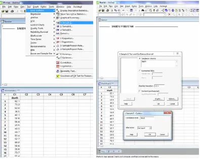
Software Solutions
Minitab
Figure 3. Minitab screen shots for constructing a confidence interval.
One-Sample Z: depth
The assumed standard deviation = 15.4
Variable N
Mean
StDev SE Mean
95% CI
depth
22
57.80
11.60
3.28
(51.36, 64.24)
Confidence Intervals about the Mean (
μ
) when the
Population Standard Deviation (
σ
) is Unknown
Typically, in real life we often don’t know the population standard deviation (σ). We can use the sample standard deviation (s) in place of σ. However, because of this change, we can’t use the standard normal distribution to find the critical values necessary for constructing a confidence interval.
35
Natural Resources Biometrics Chapter 2
Area in Right Tail
df 0.10 0.05 0.025 0.02 0.01 0.005
1 3.078 6.314 12.706 15.894 31.821 63.657 2 1.886 2.920 4.303 4.849 6.965 9.925 3 1.638 2.353 3.182 3.482 4.541 5.841 4 1.533 2.132 2.776 2.999 3.747 4.604 5 1.476 2.015 2.571 2.757 3.365 4.032
Table 2. Portion of the student’s t-table.
Ex. 4
Find the critical value
t
α2 for a 95% confidence interval with a sample size of n=13.
• Degrees of freedom (down the left-hand column) is equal to n-1 = 12
• α = 0.05 and α/2 = 0.025
• Go down the 0.025 column to 12 df
•
t
α2 = 2.179
The critical values from the students’ t-distribution approach the critical values from the standard normal distribution as the sample size (n) increases.
n Degrees of
freedom t .025
11 10 2.228
51 50 2.009
101 100 1.984
1001 1000 1.962
Table 3. Critical values from the student’s t-table.
Using the standard normal curve, the critical value for a 95% confidence interval is 1.96. You can see how different samples sizes will change the critical value and thus the confi-dence interval, especially when the sample size is small.
Construction of a Confidence Interval about
μ
when
σ
is Unknown
1)t
α2 critical value with n-1 df
2)
E t
s
n
=
α∗
2
Ex. 5
Researchers studying the effects of acid rain in the Adirondack Mountains collected water samples from 22 lakes. They measured the pH (acidity) of the water and want to construct a 99% confidence interval about the mean lake pH for this region. The sample mean is 6.4438 with a sample standard deviation of 0.7120. They do not know anything about the distribution of the pH of this population, and the sample is small (n<30), so they look at a normal probability plot.
9 8 7 6 5 4 99 95 90 80 70 60 50 40 30 20 10 5 1 pH Pe rc en t Mean 6.443 StDev 0.7120 N 22 AD 0.565 P-Value 0.127
Probability Plot of pH
Normal - 95% CI
Figure 4. Normal probability plot.
The data is normally distributed. Now construct the 99% confidence interval about the mean pH.
1)
t
α2 = 2.831
2)
E t
s
n
=
α∗
2 =
2 831
0 7120
22
.
*
.
= 0.42973)
x E
±
= 6.443 ± 0.4297The 99% confidence interval about the mean pH is (6.013, 6.863).
We are 99% confident that this interval contains the mean lake pH for this lake population.
Now construct a 90% confidence interval about the mean pH for these lakes. 1)
t
α2 = 1.721
2)
E t
s
n
=
α∗
2 =
1 721
0 7120
22
37
Natural Resources Biometrics Chapter 2
3)
x E
±
= 6.443 ± 0.2612The 90% confidence interval about the mean pH is (6.182, 6.704).
We are 90% confident that this interval contains the mean lake pH for this lake population.
Notice how the width of the interval decreased as the level of confidence decreased from 99 to 90%.
Construct a 90% confidence interval about the mean lake pH using Excel and Minitab.
Software Solutions
Minitab
One-Sample T: pH
Variable N Mean StDev SE Mean 90% CI
pH 22 6.443 0.712 0.152 (6.182, 6.704)
Additional example: www.youtube.com/watch?v=gIyPlEJE6Jc
Excel
For Excel, enter the data in the spreadsheet and select descriptive statistics. Check Summary Statistics and select the level and confidence.
Mean 6.442909
Standard Error 0.151801
Median 6.4925
Mode #N/A
Standard Deviation 0.712008 Sample Variance 0.506956
Kurtosis -0.5007
Skewness -0.60591
Range 2.338
Minimum 5.113
Maximum 7.451
Sum 141.744
Count 22
Confidence
39
Natural Resources Biometrics Chapter 2
Excel gives you the sample mean in the first line (6.442909) and the margin of error in the last line (0.26121). You must complete the computation yourself to obtain the interval (6.442909±0.26121).
Confidence Intervals about the Population
Proportion (
p
)
Frequently, we are interested in estimating the population proportion (p), instead of the population mean (μ). For example, you may need to estimate the proportion of trees in-fected with beech bark disease, or the proportion of people who support “green” products. The parameter p can be estimated in the same ways as we estimated μ, the population mean.
The Sample Proportion
• The sample proportion is the best point estimate for the true popula-tion proporpopula-tion.
• Sample proportion p xˆ=n where x is the number of elements in the sample with the characteristic you are interested in, and n is the sample size.
The Assumption of Normality when Estimating Proportions
• The assumption of a normally distributed population is still important, even though the parameter has changed.
• Normality can be verified if:
(
)
ˆ
1
ˆ
10
n p
∗ ∗ −
p
≥
Constructing a Confidence Interval about the Population Proportion
Constructing a confidence interval about the proportion follows the same three steps we have used in previous examples.
1)
Z
α2 (critical value from the standard normal table)
2)
(
)
2
ˆ 1 ˆ
p p E Z
n
α
−
= ∗ (margin of error)
3) p Eˆ± (point estimate ± margin of error)
Ex. 6
First, compute the point estimate
ˆ
.
p x
n
= =
421
=
500
0 842
Check normality: n p∗ ∗ −ˆ
(
1 pˆ)
≥10 = 500 0 842 1 0 842 66 5∗ . ∗ −(
.)
= . You can assume a normal distribution.Now construct the confidence interval: 1)
Z
α2 = 1.96
2) E Z p p
n
= α ∗
(
−)
21
ˆ ˆ =
1 96
842 1 842
500
0 032
. *
. .
.
−
(
)
=3) p Eˆ± =0 842 0 032. ±.
The 95% confidence interval for the germination rate is (81.0%, 87.4%).
We can be 95% confident that this interval contains the true germination rate for this population.
Software Solutions
Minitab
41
Natural Resources Biometrics Chapter 2
Test and CI for One Proportion
Sample X N Sample p 95% CI
1 421 500 0.842000 (0.810030, 0.873970)
Using the normal approximation.
Excel
Excel does not compute confidence intervals for estimating the population proportion.
Confidence Interval Summary
Which method do I use?
The first question to ask yourself is: Which parameter are you trying to estimate? If it is the mean (µ), then ask yourself: Is the population standard deviation (σ) known? If yes, then follow the next 3 steps:
Confidence Interval about the Population Mean (µ) when σ
is Known
1)
Z
α2)
E Z
n
=
α∗
σ
2
3)
x E
±
If no, follow these 3 steps:
Confidence Interval about the Population Mean (µ) when σ
is Unknown
1)
t
α2 critical value with n-1 df from the student t-distribution2)
E t
s
n
=
α∗
2
3)
x E
±
If you want to construct a confidence interval about the population proportion, follow these 3 steps:
Confidence Interval about the Proportion
1)
Z
α2 critical value from the standard normal table2)
E Z
p
ˆ ˆ
p
n
=
α∗
(
−
)
2
1
3) p Eˆ±
Chapter 3
Hypothesis Testing
Section 1
The previous two chapters introduced methods for organizing and summarizing sample data, and using sample statistics to estimate population parameters. This chapter introduces the next major topic of inferential statistics: hypothesis testing.
A hypothesis is a statement or claim about a property of a population.
The Fundamentals of Hypothesis Testing
When conducting scientific research, typically there is some known information, perhaps from some past work or from a long accepted idea. We want to test whether this claim is believable. This is the basic idea behind a hypothesis test:
• State what we think is true.
• Quantify how confident we are about our claim.
• Use sample statistics to make inferences about population parameters.
Hypothesis testing is a procedure, based on sample evidence and probability, used to test claims regarding a characteristic of a population.
A hypothesis is a claim or statement about a characteristic of a population of interest to us. A hypothesis test is a way for us to use our sample statistics to test a specific claim.
Ex. 1
The population mean weight is known to be 157 lb. We want to test the claim that the mean weight has increased.
Ex. 2
Two years ago, the proportion of infected plants was 37%. We believe that a treat-ment has helped, and we want to test the claim that there has been a reduction in the proportion of infected plants.
Components of a Formal Hypothesis Test
The null hypothesis is a statement about the value of a population parameter, such as the population mean (µ) or the population proportion (p). It contains the condition of equality and is denoted as H0 (H-naught).
H0 : µ = 157 or H0 : p = 0.37
The alternative hypothesis is the claim to be tested, the opposite of the null hypothesis. It contains the value of the parameter that we consider plausible and is denoted as H1 .
H1 : µ > 157 or H1 : p ≠ 0.37
The test statistic is a value computed from the sample data that is used in making a decision about the rejection of the null hypothesis. The test statistic converts the sample mean (
x
) or sample proportion (p
ˆ
) to a Z- or t-score under the assumption that the null hypothesis is true. It is used to decide whether the difference between the sample statistic and the hypothesized claim is significant.The p-value is the area under the curve to the left or right of the test statistic. It is com-pared to the level of significance (α).
The critical value is the value that defines the rejection zone (the test statistic values that would lead to rejection of the null hypothesis). It is defined by the level of significance.
The level of significance (α) is the probability that the test statistic will fall into the critical region when the null hypothesis is true. This level is set by the researcher.
45
Natural Resources Biometrics Chapter 3
important to realize that we never prove or accept the null hypothesis. We are merely saying that the sample evidence is not strong enough to warrant the rejection of the null hypothesis. The conclusion is made up of two parts:
1) Reject or fail to reject the null hypothesis, and 2) there is or is not enough evidence to support the alternative claim.
Option 1) Reject the null hypothesis (H0). This means that you have enough statistical
evidence to support the alternative claim (H1).
Option 2) Fail to reject the null hypothesis (H0). This means that you do NOT have enough evidence to support the alternative claim (H1).
Another way to think about hypothesis testing is to compare it to the US justice system. A defendant is innocent until proven guilty (Null hypothesis—innocent). The prosecuting at-torney tries to prove that the defendant is guilty (Alternative hypothesis—guilty). There are two possible conclusions that the jury can reach. First, the defendant is guilty (Reject the null hypothesis). Second, the defendant is not guilty (Fail to reject the null hypothesis). This is NOT the same thing as saying the defendant is innocent! In the first case, the prosecutor had enough evidence to reject the null hypothesis (innocent) and support the alternative claim (guilty). In the second case, the prosecutor did NOT have enough evidence to reject the null hypothesis (innocent) and support the alternative claim of guilty.
The Null and Alternative Hypotheses
There are three different pairs of null and alternative hypotheses:
Two - sided Left - sided Right-sided
H O: μ = c H O: μ = c HO: μ = c
H1: μ≠ c H1: μ < c H1: μ > c
where c is some known value.
A Two-sided Test
This tests whether the population parameter is equal to, versus not equal to, some specific value.
Ho: μ = 12 vs. H1: μ ≠ 12
Figure 1. The rejection zone for a two-sided hypothesis test.
Ex. 1
A forester studying diameter growth of red pine believes that the mean diameter growth will be different if a fertilization treatment is applied to the stand.
• Ho: μ = 1.2 in./ year
• H1: μ ≠ 1.2 in./ year
This is a two-sided question, as the forester doesn’t state whether population mean diameter growth will increase or decrease.
A Right-sided Test
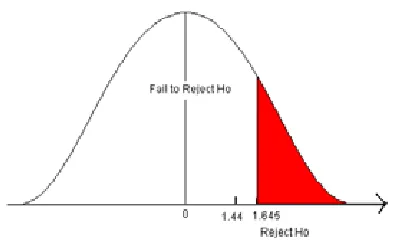
This tests whether the population parameter is equal to, versus greater than, some specific value.
Ho: μ = 12 vs. H1: μ > 12
The critical region is in the right tail and the critical value is a positive value that defines the rejection zone.
47
Natural Resources Biometrics Chapter 3
Ex. 2
A biologist believes that there has been an increase in the mean number of lakes in-fected with milfoil, an invasive species, since the last study five years ago.
• Ho: μ = 15 lakes
• H1: μ >15 lakes
This is a right-sided question, as the biologist believes that there has been an increase in population mean number of infected lakes.
A Left-sided Test
This tests whether the population parameter is equal to, versus less than, some specific value.
Ho: μ = 12 vs. H1: μ < 12
The critical region is in the left tail and the critical value is a negative value that defines the rejection zone.
Figure 3. The rejection zone for a left-sided hypothesis test.
Ex. 3
A scientist’s research indicates that there has been a change in the proportion of people who support certain environmental policies. He wants to test the claim that there has been a reduction in the proportion of people who support these policies.
• Ho: p = 0.57
• H1: p < 0.57