https://doi.org/10.5194/amt-12-3805-2019 © Author(s) 2019. This work is distributed under the Creative Commons Attribution 4.0 License.
On the information content in linear horizontal delay gradients
estimated from space geodesy observations
Gunnar Elgered1, Tong Ning2, Peter Forkman1, and Rüdiger Haas1
1Department of Space, Earth and Environment, Chalmers University of Technology, Onsala Space Observatory,
439 92 Onsala, Sweden
2Lantmäteriet (The Swedish Mapping, Cadastral and Land Registration Authority), 801 82, Gävle, Sweden
Correspondence:Gunnar Elgered ([email protected]) Received: 19 September 2018 – Discussion started: 2 October 2018 Revised: 4 June 2019 – Accepted: 21 June 2019 – Published: 12 July 2019
Abstract.We have studied linear horizontal gradients in the atmospheric propagation delay above ground-based stations receiving signals from the Global Positioning System (GPS). Gradients were estimated from 11 years of observations from five sites in Sweden. Comparing these gradients with the corresponding ones from the European Centre for Medium-Range Weather Forecasts (ECMWF) analyses shows that GPS gradients detect effects over different timescales caused by the hydrostatic and the wet components. The two stations equipped with microwave-absorbing material below the an-tenna, in general, show higher correlation coefficients with the ECMWF gradients compared to the other three stations. We also estimated gradients using 4 years of GPS data from two co-located antenna installations at the Onsala Space Ob-servatory. Correlation coefficients for the east and the north wet gradients, estimated with a temporal resolution of 15 min from GPS data, can reach up to 0.8 for specific months when compared to simultaneously estimated wet gradients from microwave radiometry. The best agreement is obtained when an elevation cut-off angle of 3◦is applied in the GPS data processing, in spite of the fact that the radiometer does not observe below 20◦. We also note a strong seasonal depen-dence in the correlation coefficients, from 0.3 during months with smaller gradients to 0.8 during months with larger gradi-ents, typically during the warmer and more humid part of the year. Finally, a case study using a 15 d long continuous very-long-baseline interferometry (VLBI) campaign was carried out. The comparison of the gradients estimated from VLBI and GPS data indicates that a homogeneous and frequent sampling of the sky is a critical parameter.
1 Introduction
Space geodetic techniques, where the fundamental observ-able is a radio signal’s time of arrival at a station on the sur-face of the Earth, are affected by variations in the propaga-tion velocity in the atmosphere. Because time measurements avoid problems related to accurate calibration, which are common for systems measuring different types of emissions, it is a common view that Global Navigation Satellite Sys-tems (GNSSs) have a long-term stability and are well suited for climate monitoring, e.g. in terms of the atmospheric wa-ter vapour content. Estimates of the total propagation delay above a GNSS station can be used to determine the inte-grated amount of water vapour. It is also common practice to estimate two-dimensional horizontal linear gradients for each station in the GNSS data processing because they im-prove the reproducibility of estimated geodetic parameters; see, e.g. Bar-Sever et al. (1998).
5.6 mm √
h−1, the weighted root-mean-square (RMS) differ-ence compared to the WVR gradients varied between 0.8 and 1.0 mm for both the GPS and the VLBI gradients. Using multi-GNSS observations, Li et al. (2015) found a signifi-cant increase in the correlation coefficient to about 0.6 when compared to ECMWF gradients, while the one for the GPS alone was typically below 0.5. In addition, they found that the RMS difference of the gradient was reduced to about 25 %– 35 % by multi-GNSS processing.
There are some interesting questions actualized by previ-ous work, which we tried to take further. Of specific inter-est in our study was to invinter-estigate if there is any systematic seasonal behaviour in the estimated gradients in Sweden and if they can be explained by the influence of regional-scale weather systems. The question about the seasonal changes of gradients was previously studied by Koulali et al. (2012). An-other issue is that comparisons of estimated GPS gradients with a high temporal resolution are rather sparse and have, to our knowledge, so far not covered periods of many years. Here we report on comparisons between GPS and WVR gra-dients, with a temporal resolution of 15 min, over a more or less continuous 4-year period. With such a resolution it is, for example, possible to study convective systems (Brenot et al., 2013) and the relation between the temporal variability of the gradients and the zenith wet delay (ZWD) during the passage of weather fronts.
In Sect. 2 we give a short background on the cause of gra-dients that are sensed by the space geodetic techniques and the model used to estimate them. In Sect. 3 instruments, tech-niques, and their data are described. The results are presented in two sections. First, in Sect. 4, we compare 11 years of to-tal gradients from five Swedish GNSS stations to gradients originating from the European Centre for Medium-Range Weather Forecasts (ECMWF) analyses. Here we study sea-sonal dependence. In Sect. 5, we use data from two co-located GNSS stations (with different antenna installations) and one WVR to assess the station performances and dif-ferences between different GPS processing variants. We also study the seasonal dependence of the estimated wet gradients over a 4-year period. Finally, within this 4-year period a 15 d long VLBI campaign occurred, which we use as a case study. In Sect. 6 we present our conclusions and suggest possible future studies of gradients.
2 Cause of horizontal gradients and models
The delay of space geodetic signals propagating through the atmosphere depends on the refractive index. For space geodetic applications it is meaningful to define one hydro-static and one wet component (Davis et al., 1985). For a hor-izontally stratified atmosphere it is then common practice to use equivalent zenith values for these components. Addition-ally we may define a horizontal linear gradient that can be in-ferred from ground-based observations (Davis et al., 1993),
consisting of one east and one north component, which in turn also can be separated into one hydrostatic and one wet component.
Hydrostatic gradients are determined by pressure and tem-perature gradients and exist mainly over regional scales (e.g. persistent high- and low-pressure systems) and syn-optic scales (e.g. weather systems). Using a European and a global GPS network, including three of the GPS stations used in this study, Meindl et al. (2004) showed that the north gradient has a clear dependence on latitude when averaged over long timescales. For the area of interest in this study, we specifically mention the Icelandic low-pressure system that typically evolves in the winter and disappears in the summer (Hewson and Longley, 1944). This is a component in the North Atlantic Oscillation and the Arctic Oscillation (Thompson and Wallace, 1998; Sanchez-Franks et al., 2016). Temperature and especially water vapour can show strong horizontal gradients over small (kilometre) scales and tem-poral variability is typically also much higher than that of the hydrostatic gradients; see, e.g. Li et al. (2015). Hence, the large local gradients over a station are mainly caused by the variability in water vapour and the wet refractivity. Gradients can be significant during a passage of a weather front; e.g. Kaˇcmaˇrík et al. (2019) report gradient amplitudes of up to 3–4 mm during the passage of an occlusion front over Germany. Nahmani et al. (2019) studied gradients during the passage of mesoscale convective systems in West Africa and Koulali et al. (2012) showed correlations between gradients and precipitation and moisture fluxes in Morocco. Other spe-cific weather phenomena that can cause horizontal variability in the partial pressure of water vapour, and hence also the wet refractivity, are sea breeze (Craig et al., 1945; Miller et al., 2003), cloud rolls (Brown, 1970), and convection processes in general.
We note that none of the known processes is expected to be strictly horizontally linear, but the strength in the geom-etry, the distribution of the observations in the sky, and the GNSS data quality makes it difficult to determine additional atmospheric parameters of a higher order.
The atmospheric parameters that are normally estimated when processing space geodesy data are an equivalent zenith wet delay and linear horizontal delay gradients in the east and the north directions. The uncertainties of the estimates depend on the geometry of the observations and the accuracy of the so-called mapping functions, used to describe the es-timated parameters dependence on the elevation angle, given the specific weather conditions at the site, at the time; see, e.g. Boehm et al. (2006) and Kaˇcmaˇrík et al. (2019). The common model used to relate the observed delay along the line-of-sight,1L(α, ε), and the estimated parameters (IERS Conventions, 2010) are also used in this study, i.e.
1L(α, ε)=mh(ε)1Lhz+mw(ε)1Lwz
wheremh,mw, andmg are the mapping functions,
depend-ing on the elevation angleε, for the hydrostatic and wet de-lays and the gradients, respectively;1Lhzand1Lwzare the
equivalent hydrostatic and wet delays in the zenith direction; αis the azimuth angle, measured clockwise from the north, implying that 4e and4n are the gradients in the east and
in the north directions. While total gradients are estimated, they can be interpreted as the sum of hydrostatic and wet components as well. In the following we will subtract the hy-drostatic component computed from ECMWF from the total GPS gradient to get the GPS wet gradient.
In addition to the east and the north gradient components, we also studied the gradient amplitude, defined as follows:
|4| =
q
42
e+42n. (2)
The gradient amplitude is defined for the hydrostatic, wet, and total gradients.
3 Instrumentation and data
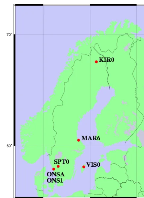
We compared gradients estimated from GPS observations acquired at five sites and six antenna and receiver instal-lations: Kiruna (KIR0), Mårtsbo (MAR6), Borås (SPT0), Visby (VIS0), and Onsala (ONSA and ONS1) with respect to VLBI, WVR, and ECMWF estimates. These stations are also part of the EUREF network (Bruyninx et al., 2012). Their geographic locations are shown in Fig. 1. In this section, we first describe the different datasets. Thereafter, we summa-rize their use and charactesumma-rize them in terms of formal errors, advantages, and disadvantages.
3.1 GPS
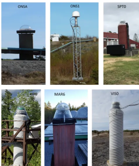
We used 11 years of GPS data (2006–2016) from the five Swedish GNSS sites mentioned above. Gradients in the east and the north directions were estimated with a temporal res-olution of 5 min. Two GNSS stations are operating continu-ously at the Onsala Space Observatory on the western coast of Sweden. The primary station, ONSA, was established in 1987 and the other station, ONS1, was taken into operation in 2011. The six antenna installations are shown in Fig. 2. The antennas of ONSA and ONS1 are located within 100 m of each other and should observe almost identical atmospheric gradients. For the time period 2013–2016, we compared gra-dients from these two stations with simultaneously estimated gradients using data from a WVR located 10 m from the ONSA antenna.
The analysis of the GPS data followed the same lines as described by Ning et al. (2013) and is summarized in Ta-ble 1. Specifically we mention that each day was analysed independently after adding 3 h of data from the previous day and 3 h from the following day, i.e. in total 30 h. The reason was to avoid discontinuities at midnight in the estimated time series.
Figure 1.The five sites used in the study. Two antenna installations, ONSA and ONS1, are co-located together with the VLBI telescope and the WVR at the Onsala site. An antenna installation is referred to as a station.
In order to investigate the impact of different constraints on the estimated gradients we also reprocessed two days of GPS data for ONSA, where large changes (2–3 mm) in both the east and the north gradient components were observed over a couple of hours by both the GPS and the WVR data. In addition to the constraint value of 0.3 mm
√
h−1suggested by Bar-Sever et al. (1998), the values 0.6, 0.9, and 1.2 mm
Figure 2.The six antenna installations used to acquire the GPS data. See Fig. 1 for their geographical location.
Recent work by Kaˇcmaˇrík et al. (2019) compared esti-mated gradients with those from a numerical weather model using different gradient mapping functions and elevation cut-off angles. They found the best agreement for an elevation cut-off angle equal to 3◦. They also showed that the Bar-Sever et al. (1998) gradient mapping function resulted in 17 % smaller gradient amplitudes compared to the Chen and Herring (1997) mapping function. For the 11-year study pre-sented in the next section, we used a 10◦ elevation cut-off angle only, whereas we used several different elevation cut-off angles in the comparison with the WVR data from the Onsala site for a 4-year period.
Based on the 5 min gradients, we calculated mean values over 15 min, 6 h, 1 d, and 1 month in order to match the tem-poral resolution of the comparison data and to study the vari-ability of the wet and the hydrostatic gradients over different timescales.
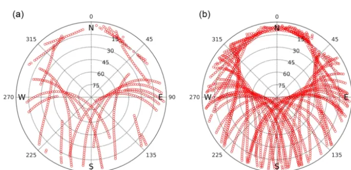
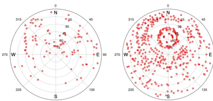
Examples of the sky coverage of the GPS observations are shown in Fig. 3 for the Onsala site. At this latitude there is a significant part of the sky that is never sampled, just north of the zenith direction. It is reasonable to assume that this will have a negative impact on the estimated gradients, especially in the north direction.
3.2 Microwave radiometer
The microwave radiometer, shown in Fig. 4, was designed in order to provide independent estimates of the wet propaga-tion delays for space geodetic applicapropaga-tions. It measures the emission from the sky, on and off the water vapour line at 22.2 GHz. Its specifications are summarized in Table 2 and the data processing was carried out as was described for an-other WVR by Elgered and Jarlemark (1998).
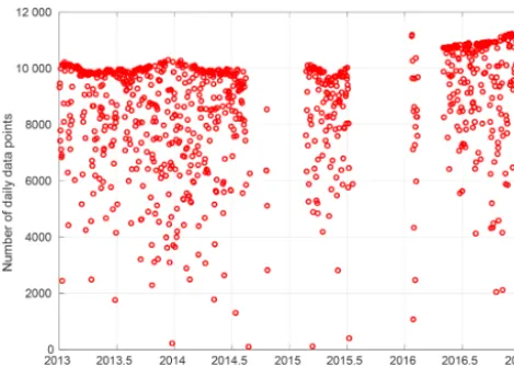
During the time period 2013–2016 the WVR was observ-ing in a sky mappobserv-ing mode, as is illustrated in Fig. 5. A dis-advantage of a WVR is that the algorithm for calculation of the wet propagation delay fails for data acquired during rain or when large liquid drops are present in the sensed atmo-sphere. Typically such conditions imply large positive errors in the wet delay and the water vapour content (Westwater and Guiraud, 1980). Therefore, data taken during rain, or when the estimated equivalent amount of liquid water in the zenith direction was>0.7 mm, were discarded from the gra-dient analysis. In addition there were also time periods when the WVR hardware failed. The amount of analysed data are shown in Fig. 6 as the number of individual observations per day. The first long data gap, in 2014–2015, was caused by a broken mechanical waveguide switch and the second long gap, in 2015–2016, was due to broken cables in the so-called cable wrap. As a consequence the cable wrap was redesigned to avoid similar failures in the future.
In order to avoid ground-noise pickup the WVR provided observations of the wet delay in the different directions above 20◦. Therefore, a simple sin(ε)mapping function was used to relate these slant wet delays to the equivalent ZWD. The WVR gradients were estimated based on all observations car-ried out during a period of 15 min using the method of least squares and the Bar-Sever gradient mapping function. We used a four-parameter model, fitting a ZWD, a ZWD rate, and an east and north gradient to the data (Davis et al., 1993). This means that the estimated gradients are independent of the successive estimates, which is different from the gradi-ents estimated from the space geodetic techniques, where temporal constraints are applied.
3.3 Very-long-baseline interferometry
Table 1.Processing of GPS data.
Parameter Description and value
Processing software GIPSY v6.2 (Webb and Zumberge, 1993)
Strategy Precise point positioning (Zumberge et al., 1997) final orbit and clock products were provided by JPL obtained from the legacy GIPSY-OASIS softwarea
Reference frame IGS08
Mapping functions for1Lz Vienna 1 2006 (VMF1) (Boehm et al., 2006)b Mapping function for4 Bar-Sever et al. (1998)
Elevation cut-off angle 10◦c
Zenith delay Estimated every 5 min, constraint 10 mm √
h−1(Jarlemark et al., 1998)
Linear horizontal gradient Estimated every 5 min, constraint 0.3 mm √
h−1(Bar-Sever et al., 1998) Ocean tide model FES2004 (Lyard et al., 2006)
Antenna phase centre igs08_1740.atx (Schmid et al., 2007)d Ambiguity resolution Yes (Bertiger et al., 2010)
Ionosphere model Second order (IGRF)e(Matteo and Morton, 2011)
aFor the 11-year dataset. For the 4-year dataset, the products were obtained from a new GipsyX software. We noted that the difference in the
products due to the change of software is small (Sibois et al., 2017).bFor the 11-year dataset. For the 4-year dataset the weighted (sin(ε)) VMF1 and the NMF (Niell, 1996) were also used.cFor the 11-year dataset. For the 4-year dataset 3 and 20◦were also used.dFor the 11-year dataset. For the 4-year dataset igs08_1869.atx was used.eInternational Geomagnetic Reference Field.
Figure 3.Sky plots of GPS observations at Onsala from 06:00 to 12:00 UT(a)and from 00:00 to 24:00 UT(b)on 12 May 2014. This particular day was chosen because it is included in the CONT14 campaign presented in Sect. 5.3. The sky distribution of observations is very similar, although not identical, for all days.
The CONT14 campaign was observed during 6– 20 May 2014. The VLBI data were analysed with the Calc/Solve analysis software (Ma et al., 1990). Station po-sitions, ZWD, atmospheric gradients, relative clock parame-ters with respect to a reference station, as well as earth rota-tion parameters were estimated. The relative clock parame-ters were estimated as piecewise linear functions every hour, with a constraint of 5×10⁻¹⁴s s−1between clock rate seg-ments. The ZWD and atmospheric gradients were estimated as piecewise linear functions (i.e. not stochastic processes) with a temporal resolution of 30 min and 6 h, respectively. Constraints for the variability of 15 mm h−1 for the ZWD rate segments and 2 mm d−1for gradient rates were applied. The NMF (Niell, 1996) mapping functions for ZWD and
the Chen and Herring (1997) mapping function for gradients were used in the analysis, together with meteorological in-formation recorded at the VLBI stations. An elevation cut-off angle of 5◦was used with no elevation-dependent weighting. Figure 7 depicts the sampling of the sky for a 6 h period, which is the highest temporal resolution of the gradient esti-mates from VLBI, as well as all observations scheduled for a 24 h experiment. This schedule was repeated every day with only minor modifications.
3.4 ECMWF
geode-Table 2.Specifications for the Konrad WVR.
Parameter Value
Frequencies 20.6 and 31.6 GHz
Antenna type (one for each channel) Conical horn with lens Antenna beam FWHM∗, E plane, ch.1 (ch.2) 2.9◦(2.0◦)
Antenna beam FWHM∗, H plane, ch.1 (ch.2) 3.4◦(2.3◦) Reference temperatures (both channels) 313 and 373 K System noise temperatures, ch.1 (ch.2) 450 K (550 K)
RF bandwidth (double sideband) 320 MHz (both channels) Absolute accuracy (weather-dependent due to the quality of tip curves) 1–3 K
Repeatability 0.1 K
∗Full width at half maximum.
Figure 4.The water vapour radiometer (WVR) Konrad at the On-sala Space Observatory.
tic sites globally. The product used here is usually referred to as LHGs (linear horizontal gradients) and is described by Boehm and Schuh (2007). It is available during certain time periods from the middle of 2005 and is more continuous from 2006. It is computed from profiles of hydrostatic and wet re-fractivity with a temporal resolution of 6 h and a spatial res-olution of 0.25◦(∼30 km). The profile closest to the site is used together with one profile to the east and one profile to the north to calculate the refractivity gradient profiles. These are thereafter integrated to give the delay gradients. Because it was observed that, on average, the gradients computed in this way overestimate the more accurate gradients estimated from slant profiles, they are scaled by empirically derived factors, 0.53 for the hydrostatic gradients and 0.71 for the wet gradients (Boehm and Schuh, 2007). This computation method and rescaling provide gradient estimates of limited accuracy but they still represent a valuable and independent
Figure 6.Number of data points per day observed by the WVR. During days without data loss, e.g. due to rain, each estimated gra-dient was based on≈100 observations in the directions illustrated in Fig. 5. Observations close to the sun were removed from the raw data before the data analysis was carried out, which causes the sea-sonal variation in the maximum number of observations per day. During the last year the measurement cycle was optimized by re-ducing some of the time delays inserted between samples, but the observational sequence shown in Fig. 5 was used during the whole period.
source of information that is used here for comparisons with estimated GPS gradients.
There are alternative methods of deriving gradients from Numerical Weather Model data using ray tracing methods; see, e.g. Zus et al. (2015), and references therein. More re-cently the Technical University of Vienna also introduced a new gradient product based on a least-squares adjustment of the ERA-Interim analyses (Landskron and Böhm, 2018).
In this study we used the LHG data from 2006 to 2016, resulting in a time series of 11 years. As an introduction, examples of the ECMWF hydrostatic and wet gradients are illustrated in Fig. 8. Worth noting is that the wet gradients dominate for the temporal resolution of 6 h and vary with the season, whereas the wet and the hydrostatic gradients show similar standard deviations (SDs) for the monthly averages.
3.5 Summary of datasets
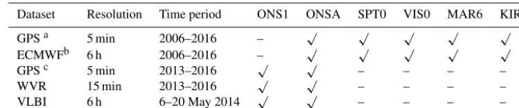
The results of comparisons between the gradients from these datasets are presented in the next two sections. The usage is defined in Table 3. In Sect. 4, GPS gradients estimated using the 10◦ elevation cut-off angle are compared to the ECMWF gradients. The temporal resolution is limited to 6 h in the ECMWF data. On the other hand, the time series are 11 years long. The results in Sect. 5 focus on comparisons of the wet gradients at the Onsala site. These have a temporal resolution of 15 min when comparing to WVR data and the ECMWF data are only used to subtract the hydrostatic gra-dients from the total gragra-dients estimated by the GPS and the
VLBI techniques. In Table 4 we summarize the typical for-mal errors of the remote-sensing techniques. Worth noting is the larger formal error for the north GPS gradient, compared to the east gradient, using the elevation cut-off angle of 20◦. The reason is that we lose many observations of satellites located in the north; see Fig. 3. Other important comments are that WVR gradients are not estimated during rain events and are not based on observations below 20◦ elevation an-gles but have a more homogeneous sky coverage compared to the GPS and the VLBI observations. Gradients from GPS and WVR have a superior temporal resolution, 5 and 15 min, respectively, compared to the 6 h resolution of the VLBI and the ECMWF gradients.
4 Comparison of gradients from GPS and ECMWF data for the time period 2006–2016
4.1 Seasonal variations in horizontal gradients
We start by investigating the characteristics of the gradients over the year. In Fig. 9 we present the monthly mean gradi-ents for the time period 2006–2016 estimated from ECMWF data and GPS data from the Onsala (ONSA) station. In the top graphs, comparing ECMWF and GPS gradients, we note that the GPS gradients show a larger variability. There are also differences between the east and the north gradients both in the mean over the year and in the seasonal variations.
We can clearly see negative north gradients in the win-ter, with a mean value around−0.2 mm, both in the GPS and the ECMWF results. When the ECMWF gradients are separated into the hydrostatic and the wet components this variation appears in the hydrostatic component. We interpret this effect as the influence of the Icelandic low-pressure sys-tem mentioned in Sect. 2. The winter feature is clearly seen in the analyses of the mean sea level pressure in the ERA-40 Atlas (https://software.ecmwf.int/static/ERA-40_Atlas/docs/ section_B/parameter_mslp.html, last access: 5 July 2019).
Figure 7.The directions of the VLBI observations for the time period from 06:00 to 12:00 UT(a)and from 00:00 to 24:00 UT(b), both on 12 May 2014.
Table 3.Summary of used datasets.
Dataset Resolution Time period ONS1 ONSA SPT0 VIS0 MAR6 KIR0
GPSa 5 min 2006–2016 – √ √ √ √ √
ECMWFb 6 h 2006–2016 – √ √ √ √ √
GPSc 5 min 2013–2016 √ √ – – – –
WVR 15 min 2013–2016 √ √ – – – –
VLBI 6 h 6–20 May 2014 √ √ – – – –
aThe GPS data were processed with elevation cut-off angles equal to 10◦.bBoehm and Schuh (2007).cThe GPS data were
processed with elevation cut-off angles equal to 3, 10, and 20◦; different mapping functions; and elevation-angle-dependent weighting.
Table 4.Formal errors of the remote-sensing techniques.
Dataset Elev. cut-off Formal error angle (◦)
Gradient ZWD
East North (mm) (mm) (mm)
GPS 3 0.14 0.13 1.7
GPS 10 0.19 0.20 2.3
GPS 20 0.35 0.43 4.0
WVR 20 0.04 0.04 0.2
VLBI 5 0.14 0.13 1.7
temporal resolution and comparisons with the WVR data in Sect. 5.
4.2 Comparing GPS and ECMWF gradients over different timescales at the five stations
We study the agreement, in terms of correlation coefficients, between the total GPS and ECMWF gradients from five GPS stations using data from 2006 to 2016. These are shown in Table 5.
The correlations seen in all cases confirm that a consistent atmospheric signal in terms of gradients is detected by the GPS observations and ECMWF analyses. We note that the correlation coefficients increase for longer-averaging time periods. Our interpretation is that by long-term averaging we compare a larger fraction of the gradient that is caused by large-scale temperature and pressure gradients. Unfortu-nately, the temporal resolution of 6 h in the ECMWF data is not sufficient to resolve either rapid changes in the pres-sure related to moving weather systems or many of the short-lived small-scale gradients associated with the variability in the water vapour.
Another result worth noting is that the two stations with the highest correlation coefficients, especially for the monthly averages, are ONSA and SPT0. The 95 % confi-dence interval is+0.03/−0.04 for the correlation coefficient of 0.90 obtained at station ONSA, based on 131 data points
(12 months over 11 years). These two stations are the only ones that are equipped with microwave-absorbing material below the antenna and above the metal plate used for the antenna mounting. This could reduce the impact from un-wanted multipath effects. The phenomenon calls for further study.
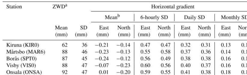
The mean values and the SD of the gradients, for the three different temporal resolutions, are presented in Tables 6 and 7 from GPS and ECMWF data, respectively. For the 6 h tempo-ral resolution, the GPS gradients estimated at the same time epoch as the ECMWF gradients are included in the calcula-tions. The daily and monthly values are averages using this 6 h data. When comparing the two tables it is clear that there are differences in the mean values of up 0.2 mm. These dif-ferences are mainly in the east component whereas there are consistent negative values for the north component. The SD of the GPS gradients is larger than the ECMWF gradients by a factor of 2. The differences may be explained using at least two reasons. First, the ECMWF gradient data used here have some intrinsic shortcomings (see Sect. 3.4). Second, not all variations in the water vapour content observed by the GPS receivers are actually represented in the ECMWF model, due to its rather coarse spatial and temporal resolutions (Bock and Parracho, 2019).
Figure 9.Monthly means of estimated gradients at the ONSA station for the period 2006–2016. The top graphs show the total gradients from ECMWF(a)and GPS(b). The graphs at the bottom show the ECMWF gradients when separated into the hydrostatic(c)and the wet gradient(d).
Table 5.Correlation coefficients for the total east and north gradients estimated from GPS data and compared to ECMWF data.
Station Six hourly Daily Monthly
East North East North East North
Kiruna (KIR0) 0.55 0.53 0.76 0.75 0.77 0.82 Mårtsbo (MAR6) 0.58 0.51 0.75 0.72 0.83 0.80 Borås (SPT0) 0.58 0.58 0.74 0.74 0.88 0.85 Visby (VIS0) 0.55 0.56 0.71 0.75 0.84 0.81 Onsala (ONSA) 0.60 0.60 0.75 0.78 0.90 0.90
5 Wet gradients at the Onsala site
For the Onsala site we study total gradients from the two GPS stations and one VLBI station and wet gradients from the WVR for the time period 2013–2016. We use the hy-drostatic gradients from ECMWF to calculate wet gradients from GPS and VLBI total gradients. The designs of the two GPS stations are different (see Fig. 2), which motivates the inclusion of both of them in the comparisons. Three differ-ent studies are made using the following data: (1) assessmdiffer-ent of the impact of using different processing of the GPS data, primarily varying the elevation cut-off angle, by compari-son to the WVR gradients; (2) using the GPS gradients from the processing variant showing the best agreement with the WVR gradients, the seasonal variations in the wet gradient are characterized; and (3) a 15 d long period with VLBI data
is used as a case study for comparisons with GPS and WVR wet gradients and the ZWD.
5.1 Test of GPS processing variants relative to WVR data
Gradients in the east and the north directions are estimated from the GPS data for five different solutions. We use three different elevation cut-off angles for the VMF1 zenith de-lay mapping functions. One additional solution is carried out with elevation-dependent weighting (sin(ε)), and in the fifth solution the VMF1 mapping functions are replaced by the NMF. As stated earlier, the gradient mapping function pre-sented by Bar-Sever et al. (1998) is used in all cases.
Table 6.Mean values and standard deviations (SDs) over the 11 years of estimated total gradients from GPS data for different temporal resolutions.
Station ZWDa Horizontal gradient
Meanb 6-hourly SD Daily SD Monthly SD
Mean SD East North East North East North East North (mm) (mm) (mm) (mm) (mm) (mm) (mm) (mm) (mm) (mm)
Kiruna (KIR0) 62 36 −0.21 −0.14 0.47 0.47 0.32 0.31 0.13 0.13 Mårtsbo (MAR6) 88 46 −0.23 −0.13 0.55 0.58 0.37 0.36 0.14 0.15 Borås (SPT0) 87 45 −0.24 −0.12 0.56 0.49 0.38 0.38 0.16 0.17 Visby (VIS0) 88 47 −0.07 −0.23 0.60 0.56 0.40 0.37 0.16 0.13 Onsala (ONSA) 92 47 0.01 −0.20 0.59 0.55 0.41 0.38 0.18 0.15
aThe zenith wet delay (ZWD) is included to illustrate the amount of water vapour in the atmosphere above the station and its SD is based on the
6 h gradients.bThe mean gradient values are based on the 6 h gradients.
Table 7.Mean values and standard deviations (SDs) over the 11 years of estimated total gradients from ECMWF data for different temporal resolutions.
Station Horizontal gradient
Mean∗ Six hourly SD Daily SD Monthly SD
East North East North East North East North (mm) (mm) (mm) (mm) (mm) (mm) (mm) (mm)
Kiruna (KIR0) 0.00 −0.14 0.28 0.26 0.20 0.19 0.07 0.07 Mårtsbo (MAR6) −0.22 −0.13 0.38 0.34 0.25 0.23 0.08 0.09 Borås (SPT0) −0.00 −0.13 0.39 0.35 0.25 0.24 0.09 0.09 Visby (VIS0) −0.01 −0.14 0.42 0.37 0.26 0.25 0.08 0.08 Onsala (ONSA) 0.03 −0.14 0.43 0.37 0.27 0.25 0.10 0.09
∗The mean gradient values are based on the 6 h gradients.
(see Fig. 8), linearly interpolated to match the time epochs of the GPS gradients, from the total GPS gradients. There-after, we form 15 min averages for the east and the north wet gradients from GPS and compare them to the corresponding WVR results.
The results for the different GPS solutions are summarized in Tables 8 and 9. Because of the different gradient ampli-tudes from the WVR and GPS, we present mean values and SD of the differences as well as correlation coefficients. Ta-ble 8 shows the results when the total gradients from the stations ONSA and ONS1 are compared to each other. Ta-ble 9 shows the results when the wet gradients from ONSA and ONS1 are compared to the WVR gradients. We note that in both tables the best agreement between the gradients es-timated is obtained for an elevation cut-off angle equal to 3◦. The 95 % confidence interval for correlation coefficients around 0.65 and approximately 80 000 data pairs is±0.004. This result was not expected by us, given that the WVR has an elevation cut-off angle of 20◦(in order to avoid ground-noise pickup) the GPS solution using the same cut-off angle would show a better agreement. Our interpretation is that for the temporal resolutions of 5–15 min, the low-elevation ob-servations are important in order to distinguish the gradient
parameters relative to other estimated parameters in the GPS analysis. A higher elevation cut-off angle will remove many observations towards the north, especially for a cut-off angle of 20◦; see Fig. 3 and Table 4 with the formal errors.
Table 8.Assessment of the different GPS solutions comparing total gradients from the two GPS stations ONSA and ONS1.
GPS Mean Standard Correlation solution differencea deviation coefficient
East North East North East North (mm) (mm) (mm) (mm)
VMF 3◦ −0.01 0.03 0.22 0.25 0.91 0.87 VMF 3◦b 0.03 0.02 0.15 0.16 0.95 0.92 NMF 3◦ −0.01 0.05 0.23 0.26 0.91 0.86 VMF 10◦ 0.02 0.04 0.25 0.27 0.91 0.88 VMF 20◦ 0.33 0.36 0.39 0.47 0.82 0.70
aThe mean difference is ONS1−ONSA.bElevation-dependent weighting, sin(ε).
Table 9.Assessment of the different GPS solutions for the wet gra-dients from the two GPS stations ONSA and ONS1 relative to the WVR data.
GPS Mean Standard Correlation solution differencea deviation coefficient
East North East North East North (mm) (mm) (mm) (mm)
ONSA
VMF 3◦ 0.23 −0.07 0.64 0.57 0.68 0.64 VMF 3◦b 0.21 −0.06 0.71 0.62 0.58 0.55 NMF 3◦ 0.22 −0.07 0.64 0.57 0.68 0.64 VMF 10◦ 0.20 −0.10 0.65 0.59 0.66 0.62 VMF 20◦ −0.02 −0.28 0.75 0.73 0.54 0.42
ONS1
VMF 3◦ 0.22 −0.04 0.64 0.58 0.68 0.64 VMF 3◦b 0.24 −0.02 0.71 0.63 0.58 0.55 NMF 3◦ 0.21 −0.02 0.64 0.58 0.68 0.63 VMF 10◦ 0.22 −0.04 0.66 0.59 0.66 0.62 VMF 20◦ 0.36 0.15 0.79 0.73 0.49 0.42
aThe mean difference is the offset referenced to the corresponding WVR time series. bElevation-dependent weighting, sin(ε).
coefficients are reduced here to 0.68 and 0.64 for the east and the north component, respectively. Since the WVR provides independent gradients, we will in the following focus on the VMF 3◦solution without elevation-dependent weighting.
5.2 Wet gradients from GPS and WVR
An overview of the data in terms of monthly means of the wet gradient amplitude and the ZWD is presented in Fig. 10. The GPS solution with a 3◦ elevation cut-off an-gle, no weighting, and the VMF1 mapping functions is used. When forming monthly means the correlations are obvious, both between GPS and WVR estimates and between the vari-ability, in terms of the SD, and the gradient amplitudes and the ZWD. Here we also note that the WVR gives much larger
Figure 10.Time series of(a)monthly means of wet gradient
ampli-tudes (
q
42e,wet+42n,wet),(b)their SD,(c)monthly means of the ZWD, and(d)the ZWD SD from GPS and WVR. The GPS results are from the 3◦solution without weighting and the temporal reso-lution in the time series used to calculate the monthly mean and the SD is 15 min. The green stars denote WVR data. The ONSA and ONS1 data are denoted by red circles and black squares, respec-tively.
gradients. Factors that can cause a difference in gradient am-plitude are listed as follows.
Table 10.The impact of the elevation cut-off angle on the estimated 15 min GPS gradient amplitude∗.
Elev. Mean gradient amplitude SD of gradient amplitude
cut-off ONSA ONS1 ONSA ONS1
angle (mm) (mm) (mm) (mm)
3◦ 0.51 0.50 0.41 0.41
10◦ 0.58 0.59 0.45 0.45
20◦ 0.75 0.70 0.45 0.46
∗The corresponding WVR values are only available for the 20◦elevation cut-off
angle: the mean is 0.87 mm and the SD is 0.78 mm.
(2) The WVR gradients for one 15 min period do not de-pend on earlier or later estimates, whereas the GPS gradi-ents are estimated using constraints on the variability. A con-straint has a similar impact as a low-pass filter (peaks with a short duration will be reduced).
(3) The fact that the WVR and the GPS gradients are com-puted for different elevation cut-off angles has two possible impacts: (i) the larger volume sensed by GPS (with a 3◦ cut-off angle) includes different air masses and introduces an av-eraging effect that reduces the mean amplitude and the vari-ability of the gradients, similar to averaging over longer time periods as shown in Table 6 and (ii) the higher cut-off angle (20◦) results in larger formal errors and thus larger variability and larger gradient amplitudes. Table 10 shows the impact of changing the elevation cut-off angle for the GPS observations for ONSA and ONS1 over the 4-year period 2013–2016. We also note from Table 4 that the formal errors of the WVR gra-dients are significantly smaller than those for the GPS gradi-ents.
We conclude that the constraints and the sampling of dif-ferent air masses are the likely explanations for the differ-ences in gradient amplitudes estimated from GPS and WVR data but cannot, based on these results, determine their rela-tive importance.
A correlation plot for the total gradients from ONSA and ONS1 for the VMF1 solution with a 3◦elevation cut-off an-gle is shown in Fig. 11. As in the previous section, we see a slightly higher correlation for the east gradients, possibly because of the poorer sampling of the sky north of the zenith direction due to the geometry of the GPS satellite constella-tion at this latitude (see Fig. 3). The two GPS staconstella-tions share several error sources, such as clock and orbit errors of the ob-served satellites, and the use of the same mapping functions, meaning that the rather high correlation is overoptimistic due to a common mode suppression of errors.
Correlation plots for the wet gradients from ONSA, ONS1, and the WVR are presented in Fig. 12. As seen previously from total gradients, the correlations between the estimated gradients from the two GPS stations are significantly higher compared to when the GPS gradients are correlated with the gradients from the WVR. It is also not surprising that the
Figure 11.Correlations between estimated total gradients from the GPS stations ONSA and ONS1 using all data with a 5 min resolu-tion from the period 2013–2016.
correlation between the wet gradients from ONSA and ONS1 are slightly lower compared to the correlation between the to-tal gradients (Fig. 11). When subtracting the hydrostatic gra-dients, a common signal is removed and the dynamic range is reduced, which affects the correlation coefficients.
The reasons for the lower correlation coefficients between the WVR and the GPS gradients are almost identical to the reasons listed above of why the WVR gradient amplitudes are higher: (1) they do not have common sources of errors; (2) the WVR data suffer both from white noise and algorithm errors, especially when liquid water is present; (3) the WVR data for each 15 min period are independent of the successive periods, whereas there are temporal constraints on the gradi-ents estimated from the GPS data; (4) the sampling of the sky also agrees much better between the two GPS stations, assuming that, in general, the directions of the observations are towards the same satellites, whereas the WVR observa-tions are evenly spread over the sky and above an elevation angle of 20◦.
Concerning the sampling of the atmosphere, the use of a multi-GNSS constellation has been shown to improve the agreement between GNSS gradients with those estimated from a WVR (Li et al., 2015). In this context it should be noted that with many more GNSS observations the optimum elevation cut-off angle may not be as low as 3◦because of an improved sampling of the atmosphere.
We investigated if an average of the wet gradients from both GPS stations, ONSA and ONS1, estimated at the same time epoch, will improve the agreement with the WVR. We see an overall small improvement. For the east gradient the individual correlation coefficients were improved from 0.678 (ONSA) and 0.682 (ONS1) to 0.698. The corresponding val-ues for the north gradient were increased from 0.639 (ONSA) and 0.635 (ONS1) to 0.666. Our interpretation is that by aver-aging the GPS gradients from ONSA and ONS1 the stochas-tic noise is reduced.
Figure 12.Correlations between estimated wet gradients from the WVR, ONSA, and ONS1 using all data from the period 2013–2016. The data in the graphs with ONSA and ONS1(a, d)have the original 5 min resolution, whereas the GPS data are averaged over 15 min when compared to the WVR data (b,eandc,f). The correlation coefficients obtained when the east gradients from the WVR were correlated with the original total gradients from GPS were 0.633 for ONSA and 0.637 for ONS1. The corresponding values for the north gradients were 0.575 for WVR-ONSA and 0.571 for WVR-ONS1. This supports our assumption that the ECMWF hydrostatic gradients are reasonably accurate when carrying out a linear interpolation between the 6 h samples.
Figure 13.Correlations between estimated wet gradients from the WVR data and the GPS data from ONSA (solid lines) and ONS1 (dotted lines), averaged over 15 min when the hydrostatic gradients are removed from the total GPS gradients for each month of the 4 years. The east gradients are presented with red lines and the north gradients with blue lines.
time periods, resulting in larger gradients and a larger dy-namic range. We note that during October 2014 there were problems with the WVR (see Fig. 6). During most of the days there is a significant data loss, likely due to rain, which could be the reason for the low correlation during this month. The
other months with low correlations are March 2015 for both the east and the north component and January and Febru-ary 2016 for the north component. In all these cases there were no large gradients detected and this has an impact on the correlations. In Fig. 8 of Lu et al. (2016), a correlation coeffi-cient of 0.52 was reported for the months March–May 2014, between GPS and WVR gradients. Here we show that the variability from month to month is large, and therefore the choice of the time period for gradient comparison studies is a critical issue.
Comparing the results obtained for ONSA with those from ONS1 they are almost identical (in both Figs. 12 and 13) meaning that in this case there is no obvious improvement from the absorbing material below the antenna on ONSA. This is different to the previous finding where ONSA and SPT0, with microwave-absorbing material, showed a better agreement with ECMWF gradients compared to the KIR0, MAR6, and VIS0 stations. Our assumption is that the lack of a concrete pillar with a metal mounting plate just below the antenna on ONS1, or any other objects affecting the electro-magnetic environment at the antenna, eliminates the need for an absorber (see Fig. 2).
5.3 GPS, VLBI, and WVR wet gradients during CONT14
Figure 14.Time series of ECMWF hydrostatic and wet gradients during the CONT14 campaign.
during the CONT14 campaign. Observations from several earlier CONT campaigns have been analysed in terms of gra-dients, with different results depending on the station and the time of the campaign (Teke et al., 2013). We use this cam-paign as an example study of the short-term variability of the wet gradients. The GPS gradients are those obtained from the VMF1 solution, unweighted, with a 3◦elevation cut-off an-gle. The ECMWF data (see Fig. 14) is only used to subtract the hydrostatic gradients from the total gradients estimated by VLBI and GPS. The time series of estimated gradients and ZWD are shown in Fig. 15.
Again we note that the size of the WVR gradients is larger compared to all other instruments. The VLBI gradients cor-relate with the gradients from the other instruments but their amplitudes are smaller. Given that the sampling of the atmo-sphere is much more sparse with the VLBI telescope, a short-lived gradient in combination with the assumption of linear functions in 6 h segments will probably reduce the variability in the estimated amplitude.
Table 11 summarizes the correlation coefficients for the east and the north VLBI wet gradients compared to those from the two GPS stations, ONSA and ONS1, and the WVR. Here we have correlated averages using data±3 h around the VLBI gradient value every 6 h. In order to be consistent the interpolated data from continuous VLBI segments are also averaged in this way.
We note that the correlation coefficients are lower for the north component for all three comparisons, whereas the SDs are similar. The reason is that the size of the east gradients are larger compared to the north gradients during this 15 d period. Scatter plots (not shown) confirm what is indicated
Table 11.Comparison of estimated wet gradients from VLBI rela-tive to GPS and WVR data.
Reference Mean Standard Correlation instrument difference∗ deviation coefficient
East North East North East North (mm) (mm) (mm) (mm)
ONSA 0.01 −0.03 0.22 0.20 0.71 0.57 ONS1 0.03 −0.08 0.22 0.20 0.71 0.56 WVR 0.30 −0.17 0.27 0.27 0.65 0.58
∗The mean difference is VLBI−reference instrument.
by the SDs: that the quality of the east and north components is similar.
Figure 15. The wet gradients and the ZWD during the VLBI CONT14 campaign 6–20 May (days 126–140). The temporal res-olution for the VLBI (blue circles) gradients is 6 h and the ZWD 30 min, 5 min for the GPS gradients for ONSA (red dots) and ONS1 (black dots), and 15 min for the WVR (green pluses).
Finally, we like to use this 15 d long time series for a dis-cussion on gradient variability. At the end of day 135 (see the ZWD plot in Fig. 15) more humid air starts to enter over the site. We note a sudden decrease, followed by a rapid in-crease. In Fig. 16 we zoom in on the gradients and the ZWD during this period. Here we have an example with wet gradi-ents from GPS and WVR gradigradi-ents when a warm front pas-sage occurs in the evening of day 135. During this paspas-sage there is also a smaller drier air mass present, causing a de-crease followed by an inde-crease in the ZWD. During this dip in ZWD the wind at the ground was from the west increasing from 7 m s−1 at 18:00 UT to 11 m s−1 at 24:00 UT. During the decrease in ZWD we see a clear positive east gradient and during the following increase in ZWD the east gradient has a negative peak. Also, during the first few hours of day 136 a decrease in the ZWD corresponds to positive values for the east gradient and the wind continued to come from the west. This is as expected, but there are also variations in the north gradient during this period, consistently detected by the WVR and the GPS data, showing that the wind at the ground was not fully representative for all altitudes.
6 Conclusions and suggestions for future work
We have estimated linear horizontal gradients from GPS data acquired at five sites in Sweden. Averaging gradients in the east and the north direction over 1 month gives cor-relation coefficients of up to 0.9 when compared to gradi-ents calculated from meteorological analyses of the ECMWF (Boehm and Schuh, 2007). The hydrostatic component gives the largest contribution to the monthly averages of the gradi-ents.
We studied wet gradients estimated with a temporal res-olution of 15 min from GPS and WVR data. We found that an elevation cut-off angle of 3◦implies a better agreement when comparing GPS gradients with those from the WVR, in spite of the fact that the WVR does not observe the atmo-sphere below elevation angles of 20◦. This confirms the re-sult from Kaˇcmaˇrík et al. (2019) showing that low-elevation observations are important for the accuracy of the estimated GPS gradients, although none of us have shown that 3◦is an optimum cut-off angle.
We also note that when using a 3◦elevation cut-off angle in the GPS processing, the amplitude of the GPS gradients decreases by approximately 20 % compared to using a 20◦ cut-off angle. We interpret this decrease as the result of two combined effects: (1) the decrease in mean amplitude and variability at the lower cut-off angle results from the aver-aging of a larger air mass (similar to averaver-aging over longer periods); (2) the increase in mean amplitude and variability at the higher cut-off angle results from the increase in un-certainty and thus larger scatter in the estimates. The relative importance of these two effects are recommended topics to be studied further, e.g. by using simulations based on high-resolution numerical weather models.
Correlation coefficients between wet gradients estimated from GPS and the WVR data can reach up to 0.8 for specific months. We note a strong seasonal dependence, from 0.3 dur-ing months with smaller gradients to 0.8 durdur-ing months with larger gradients, typically during the warmer and more humid part of the year. Related to this we suggest further studies of large wet gradients estimated from GPS, again in combina-tion with meteorological high-resolucombina-tion models for verifica-tion of the quality of the gradients.
In general, we also note slightly higher correlation coeffi-cients for the GPS-derived gradients in the east compared to the north direction. We interpret this difference to be caused by an inhomogeneous spatial sampling of the sky, which is important when we assume that the linear model describing horizontal gradients has deficiencies. The different sampling of the sky is an important issue for any comparison between different techniques. This question remains unresolved and is also recommended for further study.
Figure 16.Zoom in on the time series in Fig. 15. The symbols are as before: VLBI gradients (blue circles), GPS gradients for ONSA (red dots) and ONS1 (black dots), and WVR (green pluses).
higher orbit inclination will reduce the part of the sky not sampled by GPS.
For VLBI the use of VGOS (twin) telescopes will also dra-matically improve the sampling of the atmosphere. When WVR data are used to evaluate gradients from the space geodetic techniques one may consider also applying differ-ent constraints on the temporal variability of these estimates. We suggest that future work on gradients should focus on the interplay between the elevation cut-off angle, the tempo-ral resolution, and the constraint value using both single and multi-GNSS. Furthermore, we believe that the outcome of such studies will be weather- and site-dependent, which will make it difficult to arrive at just one optimal recommendation that is globally valid.
Data availability. The input GNSS data, in RINEX format, are available from EUREF: https://igs.bkg.bund.de/dataandproducts/ browse (last access: 8 July 2019). The input VLBI data are avail-able from the IVS: ftp://ivs.bkg.bund.de/pub/vlbi/ivsdata/db/2014/ (last access: 8 July 2019). The ECMWF gradients are accessible from the Technical University of Vienna: http://vmf.geo.tuwien.ac. at/trop_products/GNSS/LHG/ (last access: 8 July 2019). The esti-mated gradients from GPS, VLBI, and WVR data have been reg-istered and archived by the Swedish National Data Service (SND): https://doi.org/10.5878/nswt-yr39 (Elgered et al., 2019).
Author contributions. GE coordinated and wrote the major part of the manuscript and together with TN planned the different GNSS data analyses during the COST Action ES1206. TN performed the GNSS data analyses, resulting in the estimated gradients. PF and
RH carried out the same task for WVR and VLBI data, respectively. All authors contributed in the writing process, to the sections pre-senting the results produced by each author in particular, and ap-proved the entire paper before submission.
Competing interests. The authors declare that they have no conflict of interest.
Special issue statement. This article is part of the special issue “Ad-vanced Global Navigation Satellite Systems tropospheric products for monitoring severe weather events and climate (GNSS4SWEC) (AMT/ACP/ANGEO inter-journal SI)”. It is not associated with a conference.
Acknowledgements. We appreciate the constructive comments and suggestions from the editor and the three referees. They resulted in a significantly improved paper, offering additional possible expla-nations for the obtained results as well as additional studies. For example, the use of a 3◦elevation cut-off angle in the GPS data processing was not included in our original manuscript. The map in Fig. 1 was produced using Generic Mapping Tools (Wessel and Smith, 1998).
References
Bar-Sever, Y.-E., Kroger, P. M., and Börjesson, J. A.: Esti-mating horizontal gradients of tropospheric path delay with a single GPS receiver, J. Geophys. Res., 103, 5019–5035, https://doi.org/10.1029/97jb03534, 1998.
Bertiger, W., Desai, S. D., Haines, B., Harvey, N., Moore, A. W., Owen, S., and Weiss, J. P.: Single receiver phase am-biguity resolution with GPS data, J. Geod., 84, 327–337, https://doi.org/10.1007/s00190-010-0371-9, 2010.
Bock, O. and Parracho, A. C.: Consistency and representativeness of integrated water vapour from ground-based GPS observa-tions and ERA-Interim reanalysis, Atmos. Chem. Phys. Discuss., https://doi.org/10.5194/acp-2019-28, in review, 2019.
Boehm, J., Werl, B., and Schuh, H.: Troposphere mapping functions for GPS and very long baseline interferometry from European Centre for Medium-Range Weather Forecasts operational analysis data, J. Geophys. Res., 111, B02406, https://doi.org/10.1029/2005JB003629, 2006.
Boehm, J. and Schuh, H.: Troposphere gradients from the ECMWF in VLBI analysis, J. Geod., 81, 403–408, https://doi.org/10.1007/s00190-007-0144-2, 2007.
Brenot, H., Neméghaire, J., Delobbe, L., Clerbaux, N., De Meut-ter, P., Deckmyn, A., Delcloo, A., Frappez, L., and Van Roozendael, M.: Preliminary signs of the initiation of deep convection by GNSS, Atmos. Chem. Phys., 13, 5425–5449, https://doi.org/10.5194/acp-13-5425-2013, 2013.
Brown, R. A.: A secondary flow model for the planetary boundary layer, J. Atmos. Sci., 27, 742–757, 1970.
Bruyninx, C., Habrich, H., Söhne, W., Kenyeres, A., Stangl, G., and Völksen, C.: Enhancement of the EUREF Permanent Network Services and Products, Geodesy for Planet Earth, IAG Symposia Series, 136, 27–35, https://doi.org/10.1007/978-3-642-20338-1_4, 2012.
Chen, G. and Herring, T. A.: Effects of atmospheric azimuthal asymmetry on the analysis of space geodetic data, J. Geophys. Res., 102, 20489–20502, https://doi.org/10.1029/97JB01739, 1997.
Craig, R. A., Katz, I., and Harney, P. J.: Sea breeze cross sections from pyschrometric measurements, B. Am. Meteorol. Soc., 26, 405–410, 1945.
Davis, J. L., Herring, T. A., Shapiro, I. I., Rogers, A. E. E., and Elgered, G.: Geodesy by radio interferometry: Effects of atmo-spheric modeling errors on estimates of baseline length, Radio Sci., 20, 1593–1607, https://doi.org/10.1029/RS020i006p01593, 1985.
Davis, J. L., Elgered, G., Niell, A. E., and Kuehn, C. E.: Ground-based measurement of gradients in the “wet” radio refractivity of air, Radio Sci., 28, 1003–1018, https://doi.org/10.1029/93RS01917, 1993.
Elgered, G. and Jarlemark, P. O. J.: Ground-Based Mi-crowave Radiometry and Long-Term Observations of Atmospheric Water Vapor, Radio Sci., 33, 707–717, https://doi.org/10.1029/98RS00488, 1998.
Elgered, G., Forkman, P., Haas, R., and Ning, T.: Chalmers Uni-versity of Technology, Department of Space, Earth and Envi-ronment, On the information content in linear horizontal delay gradients estimated from space geodesy observations, Swedish National Data Service, Version 1.0, https://doi.org/10.5878/nswt-yr39, 2019.
Gradinarsky, L. P., Haas, R., Elgered, G., and Johansson, J. M.: Wet path delay and delay gradients inferred from microwave ra-diometer, GPS and VLBI observations, Earth Planets Space, 52, 695–698, https://doi.org/10.1186/BF03352266, 2000.
Haas, R., Hobiger, T., Kurihara S., and Hara, T.: Ultra-rapid earth rotation determination with VLBI dur-ing CONT11 and CONT14, J. Geod., 91, 831–837, https://doi.org/10.1007/s00190-016-0974-x, 2017.
Hewson, E. W. and Longley, R. W.: Meteorology: Theoretical and Applied, John Wiley & Sons, New York, 1944.
IERS Conventions: IERS Technical Note, edited by: Petit, G. and Luzum, B.; 36, Verlag des Bundesamts für Kartographie und Geodäsie, Frankfurt am Main, 179 pp., 2010.
Jarlemark, P. O. J., Emardson, T. R., and Johansson, J. M.: Wet De-lay Variability Calculated from Radiometric Measurements and Its Role in Space Geodetic Parameter Estimation, Radio Sci., 33, 719–730, https://doi.org/10.1029/98RS00551, 1998.
Kaˇcmaˇrík, M., Douša, J., Zus, F., Václavovic, P., Balidakis, K., Dick, G., and Wickert, J.: Sensitivity of GNSS tropospheric gradients to processing options, Ann. Geophys., 37, 429–446, https://doi.org/10.5194/angeo-37-429-2019, 2019.
Koulali, A., Ouazar, D., Bock, O., and Fadil, A.: Study of seasonal-scale atmospheric water cycle with ground-based GPS receivers, radiosondes and NWP models over Morocco, Atmos. Res., 104– 105, 273–291, https://doi.org/10.1016/j.atmosres.2011.11.002, 2012.
Landskron, D. and Böhm, J.: Refined discrete and empirical hor-izontal gradients in VLBI analysis, J. Geod., 92, 1387–1399, https://doi.org/10.1007/s00190-018-1127-1, 2018.
Li, X., Zus, F., Lu, C., Ning, T., Dick, G., Ge, M., Wickert, J., and Schuh, H.: Retrieving high-resolution tropospheric gradi-ents from multiconstellation GNSS observations, Geophys. Res. Lett., 42, 4173–4181, https://doi.org/10.1002/2015GL063856, 2015.
Lu, C., Li, X., Li, Z., Heinkelmann, R., Nilsson, T., Dick, G., Ge, M., and Schuh, H.: GNSS tropospheric gradi-ents with high temporal resolution and their effect on pre-cise positioning, J. Geophys. Res.-Atmos., 121, 912–930, https://doi.org/10.1002/2015JD024255, 2016.
Lyard, F., Lefevre, F., Letellier, T., and Francis, O.: Modelling the global ocean tides: Modern insights from FES2004, Ocean Dy-nam., 56, 394–415, https://doi.org/10.1007/s10236-006-0086-x, 2006.
Ma, C., Sauber, J. M., Bell, L. J., Clark, T. A., Gor-don, D., Himwich, W. E., and Ryan, J. W.: Measure-ment of horizontal motions in Alaska using very long baseline interferometry, J. Geophys. Res., 95, 21991–2011, https://doi.org/10.1029/JB095iB13p21991, 1990.
MacMillan, D. S.: EOP and scale from continuous VLBI observing: CONT campaigns to future VGOS networks, J. Geod., 91, 819– 829, https://doi.org/10.1007/s00190-017-1003-4, 2017. Matteo, N. A. and Morton, Y. T.: Ionosphere geomagnetic
field: Comparison of IGRF model prediction and satel-lite measurements 1991–2010, Radio Sci., 46, RS4003, https://doi.org/10.1029/2010RS004529, 2011.
Miller, S. T. K., Keim, B. D., Talbot, R. W., and Mao, H.: Sea breeze: Structure, forecasting, and impacts, Rev. Geophys., 41, 1011, https://doi.org/10.1029/2003RG000124, 2003.
Nahmani, S., Bock, O., and Guichard, F.: Sensitivity of GPS tropospheric estimates to mesoscale convective systems in West Africa, Atmos. Chem. Phys. Discuss., https://doi.org/10.5194/acp-2018-1242, in review, 2019. Niell, A. E.: Global mapping functions for the atmosphere
de-lay at radio wavelengths, J. Geophys. Res., 101, 3227–3246, https://doi.org/10.1029/95JB03048, 1996.
Niell, A., Barrett, J., Burns, A., Cappallo, R., Corey, B., Derome, M., C. Eckert, C., Elosegui, P., McWhirter, R., Poirier, M., Ra-jagopalan, G., Rogers, A., Ruszczyk, C., SooHoo, J., Titus, M., Whitney, A., Behrend, D., Bolotin, S., Gipson, J., Gordon, D., Himwich, E., and Petrachenko, B.: Demonstration of a broad-band very long baseline interferometer system: A new instrument for high-precision space geodesy, Radio Sci., 53, 1269–1291, https://doi.org/10.1029/2018RS006617, 2018.
Ning, T., Elgered, G., Willén, U., and Johansson, J. M.: Evalua-tion of the atmospheric water vapor content in a regional climate model using ground-based GPS measurements, J. Geophys. Res., 118, 1–11, https://doi.org/10.1029/2012JD018053, 2013. Nothnagel, A., Artz, T., Behrend, D., and Malkin, Z.: International
VLBI Service for Geodesy and Astrometry Delivering high-quality products and embarking on observations of the next gen-eration, J. Geod., 91, 711–721, https://doi.org/10.1007/s00190-016-0950-5, 2017.
Sanchez-Franks, A., Hameed, S., and Wilson, R. E.: The Icelandic Low as a Predictor of the Gulf Stream North Wall Position, J. Phys. Oceanogr., 46, 817–826, https://doi.org/10.1175/JPO-D-14-0244.1, 2016.
Schmid, R., Steigenberger, P., Gendt, G., Ge, M., and Rothacher, M.: Generation of a consistent absolute phase center correction model for GPS receiver and satellite antennas, J. Geod., 81, 781– 798, https://doi.org/10.1007/s00190-007-0148-y, 2007.
Sibois, A., Amiri, N., Bertiger, W., Miller, M., Murphy, D., Ries, P., Sakamura, C., and Sibthorpe, A.: Ensuring a smooth operational transition from GIPSY-OASIS to GipsyX: product verification and validation overview, poster presented at the IGS Work-shop, Paris, France, available at: http://www.igs.org/presents/ workshop2017 (last access: 5 July 2019), 2017.
Teke, K., Nilsson, T., Böhm, J., Hobiger, T., Steigenberger, P., Garcia-Espada, S., Haas, R., and Willis, P.: Tropo-sphere delays from space geodetic techniques, water va-por radiometers, and numerical weather models over a se-ries of continuous VLBI campaigns, J. Geod., 87, 981–1001, https://doi.org/10.1007/s00190-013-0662-z, 2013.
Thompson, D. W. J. and Wallace, J. M.: The Arctic oscil-lation signature in the wintertime geopotential height and temperature fields, Geophys. Res. Lett., 25, 1297–1300, https://doi.org/10.1029/98GL00950, 1998.
Webb, F. H. and Zumberge, J. F.: An Introduction to the GIPSY/OASIS-II, JPL Publ., D-11088, Jet Propulsion Labora-tory, Pasadena, California, 1993.
Wessel, P. and Smith, W. H. F.: New, improved version of generic mapping tools released, EOS T. Am. Geophys. U., 79, 579, https://doi.org/10.1029/98EO00426, 1998.
Westwater, E. R. and Guiraud, F. O.: Ground-based microwave radiometric retrieval of precipitable water vapor in presence of clouds with high liquid content, Radio Sci., 15, 947–957, https://doi.org/10.1029/RS015i005p00947, 1980.
Zumberge, J. F., Heflin, M. B., Jefferson, D. C., Watkins, M. M., and Webb, F. H.: Precise point positioning for the efficient and robust analysis of GPS data from large networks, J. Geophys. Res., 102, 5005–5017, https://doi.org/10.1029/96JB03860, 1997.