https://doi.org/10.5194/cp-15-2031-2019 © Author(s) 2019. This work is distributed under the Creative Commons Attribution 4.0 License.
A 120 000-year record of sea ice in the North Atlantic?
Niccolò Maffezzoli1,2, Paul Vallelonga2, Ross Edwards3,4, Alfonso Saiz-Lopez5, Clara Turetta1,6, Helle Astrid Kjær2, Carlo Barbante1,6, Bo Vinther2, and Andrea Spolaor1,6
1Institute of Polar Sciences, ISP-CNR, Via Torino 155, 30172 Venice, Italy
2Physics of Ice, Climate and Earth (PICE), Niels Bohr Institute, University of Copenhagen, Tagensvej 16,
2200 Copenhagen, Denmark
3Physics and Astronomy, Curtin University of Technology, Kent St, Bentley, WA 6102, Perth, Australia 4Department of Civil and Environmental Engineering, UW-Madison, Madison, WI 53706, USA
5Department of Atmospheric Chemistry and Climate, Institute of Physical Chemistry Rocasolano, CSIC, Madrid, Spain 6Department of Environmental Sciences, Informatics and Statistics,
Ca’ Foscari University of Venice, Via Torino 155, 30170 Venice, Italy
Correspondence:Niccolò Maffezzoli (niccolo.maffezzoli@unive.it)
Received: 2 July 2018 – Discussion started: 17 July 2018
Revised: 2 November 2019 – Accepted: 15 November 2019 – Published: 19 December 2019
Abstract.Although it has been demonstrated that the speed and magnitude of the recent Arctic sea ice decline is un-precedented for the past 1450 years, few records are avail-able to provide a paleoclimate context for Arctic sea ice ex-tent. Bromine enrichment in ice cores has been suggested to indicate the extent of newly formed sea ice areas. De-spite the similarities among sea ice indicators and ice core bromine enrichment records, uncertainties still exist regard-ing the quantitative linkages between bromine reactive chem-istry and the first-year sea ice surfaces. Here we present a 120 000-year record of bromine enrichment from the RE-CAP (REnland ice RE-CAP) ice core, coastal east Greenland, and interpret it as a record of first-year sea ice. We compare it to existing sea ice records from marine cores and tenta-tively reconstruct past sea ice conditions in the North At-lantic as far north as the Fram Strait (50–85◦N). Our inter-pretation implies that during the last deglaciation, the transi-tion from multi-year to first-year sea ice started at∼17.5 ka, synchronously with sea ice reductions observed in the east-ern Nordic Seas and with the increase in North Atlantic ocean temperature. First-year sea ice reached its maximum at 12.4–11.8 ka during the Younger Dryas, after which open-water conditions started to dominate, consistent with sea ice records from the eastern Nordic Seas and the North Icelandic shelf. Our results show that over the last 120 000 years, multi-year sea ice extent was greatest during Marine Isotope Stage (MIS) 2 and possibly during MIS 4, with more extended
first-year sea ice during MIS 3 and MIS 5. Sea ice extent during the Holocene (MIS 1) has been less than at any time in the last 120 000 years.
1 Introduction:Brenras a potential indicator of past
sea ice conditions
The connection between Arctic sea ice and bromine was first identified through an anticorrelation between spring-time ground level ozone (O3) and filterable bromine air
date, both model studies (Yang et al., 2008, 2010) and ex-perimental evidence (Pratt et al., 2013; Zhao et al., 2016; Frey et al., 2019) consider the deposited snow layer on FYSI (known as salty blowing snow) to be the most efficient sub-strate for SSA release and bromine activation.
Atmospheric bromine and sodium thus originate from both oceanic and FYSI sea-salt aerosols, where their concentra-tion ratio is that of seawater mass: (Br/Na)m =0.0062 (the
subscript indicates “marine”, Millero et al., 2008). Brenr
val-ues in ice core records, i.e. the bromine-to-sodium mass ra-tios beyond the seawater value (Eq. 1), were introduced by Spolaor et al. (2013b) as a potential proxy for past FYSI con-ditions within the ocean region influencing the ice core loca-tion. The basic assumption behind this idea is that bromine recycling on FYSI surfaces would increase the bromine-to-sodium mass ratio beyond the seawater value in the atmo-sphere and at the ice core location, thus isolating the effect of FYSI-induced bromine recycling from the sea-salt aerosol contribution, the latter being interfered with by oceanic emis-sions. Further studies have provided some evidence on the validity of Brenras an FYSI indicator (Spolaor et al., 2013a,
2014, 2016a). At present, however, this interpretation is still challenged by several uncertainties related to the different variables which play a role in the chemical and physical pro-cesses involved (Abbatt, 2013). These can be grouped into three categorizes: bromine activation, transport, and deposi-tion or postdeposideposi-tion. They are briefly discussed here and in Appendix A.
Pratt et al. (2013) showed that saline snow collected on Arctic tundra or first-year sea ice surfaces can serve as an ef-ficient reservoir for bromine activation. They point out, how-ever, that the acidity of snow is a prerequisite for bromine ac-tivation, as well as internal snowpack air chemistry (e.g. the concentration of·OH, NO−3/NO−2). A modification in these factors would alter the bromine production efficiency at con-stant FYSI extent. Aged sea ice (second-year sea ice or older) possibly contributes to bromine activation due to a non-zero salt content, but the amount of this second-order source effect is unknown.
Bromine travels from the source region to the ice core location both in the aerosol and gas phases, while sodium is only found in the aerosol phase. To date, the partition-ing of bromine species between the two phases is not clear. Additionally, some studies have reported that bromine recy-cling takes place within the plume even during the transport (Zhao et al., 2016), leading to possible bromine depletion from the aerosol in favour to the gas phase. Overall, the fi-nal observed Brenrvalues in ice samples depend on the
rela-tive importance of aerosol and gas-phase bromine partition-ing. It appears that fine aerosols are enriched in bromine, while coarse particles are depleted (Legrand et al., 2016, Theodore Koenig, personal communication, 2018). Addi-tionally, the two phases likely have a different atmospheric residence time; thus, the final bromine-to-sodium ratio found in the snow might be a function of the transport duration.
In general, bromine-reactive surfaces would increase the at-mospheric residence time of bromine species, enhancing the bromine-to-sodium ratios away from the sea ice or ocean sources. On this topic, from springtime Arctic snow sam-ples collected from a transect directed inland, Simpson et al. (2005) showed that sodium is deposited faster than bromine, suggesting a role of longer-lasting gas-phase bromine (Fig. 3 in their study). From samples collected during a coast-to-inland Antarctic transect (Zhongshan Station–Dome A), Li et al. (2014) showed much reduced spatial gradients between sodium and bromine snow concentrations when compared to Simpson and co-workers (Fig. 2 in Li et al., 2014). In a sim-ilar inland-directed Antarctic transect (Talos Dome–Dome C), Spolaor et al. (2013b) presented simultaneous bromine and sodium deposition fluxes from three sites and a model run aimed at explaining the experimental results (Fig. 6 in their study). The authors note that for their results to be ex-plained by the model, the deposition velocity of HBr needs to be set at least 3 times larger than the average sea-salt aerosol deposition velocity. To conclude, the interference of transport processes with the sea ice source effects in either the Arctic or Antarctica is not clear and should be further investigated.
The last set of uncertainties relates to the variables asso-ciated with the deposition of bromine and sodium, such as the variability in accumulation rates over long timescales, which would impact the relative importance of the wet and dry contributions of the two species. Finally, photolytic re-emission of bromine from the snowpack could be responsi-ble for bromine loss and decreased Brenrvalues. A dedicated
discussion of this last topic can be found in Appendix A. We acknowledge the above-mentioned open questions on the validity of Brenras an FYSI proxy and clearly point out
that further studies are needed to shed light on these uncer-tainties. We thus proceed with the interpretation of Brenras
an FYSI proxy bearing in mind that other variables could, at present, explain a Brenrrecord.
Here, we consider the available evidence regarding past sea ice conditions in the North Atlantic and present a bromine enrichment record from the RECAP (REnland ice CAP) ice core, located in coastal east Greenland. Because of its lo-cation, RECAP should record the fingerprint of sea ice in the North Atlantic. We compare our RECAP Brenr record
with sea ice reconstructions from five marine sediment cores drilled within the Renland source area: the Fram Strait, the Norwegian Sea and the North Icelandic shelf (Fig. 1).
2 Methods
2.1 The 2015 RECAP ice core
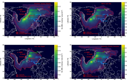
Figure 1.Modern (2000–2016) source region of atmospheric sodium and bromine deposited at the Renland site estimated from 3 d back trajectory calculations. On thezaxis is represented the number of marine boundary layer (MBL) crossings per unit area, derived by selecting only those trajectories which crossed the 900 hPa isosurface for at least 10 h (see Sect. 2.3). The red line contours 75 % of the distribution integral, and it is considered to be the bromine and sodium source region. It covers the North Atlantic Ocean from∼50 to 85◦N. A minor contribution is expected from west Greenland waters. Note that areas outside the 75 % line with counts<0.02 crossings km−2 are not coloured. The analysis is performed on a seasonal basis. The Renland ice cap is marked with a star; the NEEM and NGRIP core sites are marked with a circle. The diamonds indicate the marine cores discussed in the text: Svalbard margin (MSM5/5-712-2, Müller and Stein, 2014), North Icelandic shelf (MD99-2272, Xiao et al., 2017) and the Norwegian Sea (JM11-FI-19PC, Hoff et al., 2016; MD99-2272, Muschitiello et al., 2019; JM99-1200, Cabedo-Sanz et al., 2013).
was recovered to 584 m (bedrock). The drilling occurred in a dry borehole to 130 m depth, and estisol 140 drilling fluid was used for the remaining depth. The record covers the last 120 800 years. The core age model is described in full details in the Supplement of Simonsen et al. (2019).
The ice core samples dedicated to mass spectroscopy mea-surements (n=1205) were collected and automatically de-contaminated by a continuous ice core melting system as part of the RECAP Continuous Flow Analysis (CFA) campaign conducted at the University of Copenhagen in Autumn 2015. The ice core was melted at a speed of approx. 3 cm min−1 on a gold-coated plate copper melter head (Bigler et al., 2011; Kaufmann et al., 2008). Meltwater was collected con-tinuously from the melter head into polyethylene vials pre-cleaned with ultrapure water (>18.2 Mcm−1) at two dif-ferent depth resolutions. From the ice cap surface to a depth of 535.15 m, samples incorporated ice meltwater spanning depths of 55 cm. From a depth of 535.15 m to the ice cap
bedrock, the samples integrated 18.3 cm. The time resolu-tion is annual to multicentennial in the Holocene and centen-nial to millencenten-nial in the glacial section. After collection, the samples were immediately refrozen at−30◦C and kept in the dark until mass spectroscopy analyses to reduce bromine photolysis reactions.
2.2 Ice core measurements: determination of Br, Na, Cl, Ca and Mg
The depth and age ranges associated with the Italian samples are surface–150 m (2015 CE–328 years b2k), 165– 219 m (383–636 years BP), 234–413 m (727–2857 years b2k) and 441–495 m (3522–5749 years b2k). The depth and age ranges associated with the Australian samples are 150– 165 m (328–383 years b2k), 219–234 m (636–727 years b2k), 413–441 m (2857–3522 years b2k) and 495–562 m (5749– 120 788 years b2k).
University Ca’ Foscari of Venice, Italy. Bromine and sodium (79Br and 23Na) were determined by collision re-action cell inductively coupled plasma mass spectroscopy (CRC-ICP-MS, Agilent 7500cx, Agilent, California, USA). The introduction system consisted of an ASX-520 autosam-pler (CETAC Technologies, Omaha, USA) and Scott spray chamber fitted with a MicroFlow PFA (perfluoroalkoxy) nebulizer. The sample flow was kept at 100 µL min−1. All reagents and standard solutions were prepared with ultra-pure water (UPW; 18.2 Mcm−1). Nitric acid (65 %v/v,
trace metal grade, Romil, Cambridge, UK) and UPW washes (2 min each) were used for background recovery after every sample analysis. The nitric acid washing concentration was lowered to 2 %. The experimental routine (standards and cal-ibrations) as well as the overall instrument performance (de-tection limits and reproducibility) are the same as in Spolaor et al. (2016b).
Curtin University of Technology, Perth, Australia. The analyses were performed by inductively coupled plasma sec-tor field mass spectroscopy in reverse Nier–Johnson geom-etry (ICP-SFMS, Element XR, Thermo Fisher, Germany) inside a Class 100 clean room environment at the Curtin University TRACE facility (Trace Research Advanced Clean Environment Facility). The ICP-SFMS introduction system consisted of an Elemental Scientific Inc. (ESI, Omaha, USA) syringe-pumped autosampler (Seafast II) with a 1 mL PFA capillary injection loop and using an ultrapure water car-rier. A 1 ppb indium internal standard in 5 % v/v nitric acid (HNO3, double-PFA distilled) was mixed inline at a
flow rate of 25 µL min−1 using a T-split (final flow rate of 400 µL min−1, take-up time 1.5 min). Nebulization occurred in a peltier cooled (2◦C) quartz cyclonic spray chamber (PC3, ESI), fitted with a PFA micro-concentric nebulizer (PFA-ST, ESI). Bromine, sodium, magnesium, chlorine and calcium isotopes (79Br,23Na, 24Mg, 35Cl, 44Ca) were de-tected in medium resolution (10 % valley resolution of 4000 amu) and normalized to 115In. Memory effects were re-duced by rinsing the system between samples with high-purity HNO3(3 %) and UPW. One procedural blank and one
quality-controlled standard (QC) were analysed every five samples to monitor the system stability. The detection limits, calculated as 3σ of the blank values (n=80) were 0.18 ppb (Br), 1.1 ppb (Na), 0.2 ppb (Mg), 1.6 ppb (Ca) and 4.6 ppb (Cl). The majority of the sample concentrations were above the detection limits for all elements (>97 %). The relative standard deviations of the control standard sample (n=82) concentrations were monitored over >100 h and were 9 %
(Br), 4 % (Na), 3 % (Mg), 4 % (Ca) and 13 % (Cl). Calibra-tion standards were prepared by sequential diluCalibra-tion (seven standards) of NIST traceable commercial standards (High-Purity Standards, Charleston, USA). All materials used for the analytical preparations were systematically cleaned with UPW (18.2>Mcm−1) and double-PFA distilled ultrapure HNO3(3 %, prepared from IQ grade HNO3, Choice
Analyt-ical Pty Ltd, Australia) throughout.
A laboratory intercomparison between sodium and bromine measurements was performed on a common set of samples (n=140) to investigate differences between the an-alytical techniques and laboratories, as described in Valle-longa et al. (2017). The correlations and the gradients be-tween the measured concentrations in the two set-ups are ρ(NaIT-NaAUS)=0.99 (n=140;p <0.01),mNa=1.08±
0.01 (1σ) for sodium andρ(BrIT-BrAUS)=0.93 (n=140;
p <0.01),mBr=1.08±0.02 (1σ) for bromine.
Figure 2.Map of modern Arctic sea ice age shown in representative extreme conditions: winter maximum (February 1987,a) and summer minimum (September 2012,b). The marine cores discussed in the text are indicated by coloured diamonds. See Fig. 1 for the marine core names and references. The sea ice age data are from NSIDC/NASA (v.3) (Tschudi et al., 2016).
overall interpretation of the RECAP record, the source area is therefore assumed to be the 75 % contour region of the residence time analysis end point distribution (Fig. 1). Such a region is nowadays mostly dominated by open-water (OW) conditions, with only minor contributions of FYSI grown in situ and multi-year sea ice (MYSI) transported south of the Arctic Ocean alongside the east Greenland coastline via the Transpolar Drift (Fig. 2).
3 Calculation of bromine enrichment (Brenr) and
Brenrtime series
The bromine enrichment values in the ice samples are cal-culated from the departure from the seawater abundance, the latter inferred from sodium (hereafter sea-salt sodium, ssNa), Eqs. (1), (2):
Brenr=
Br/ssNa (Br/Na)m
, (1)
Na=ssNa+nssNa, (2)
where Br, ssNa and nssNa are the bromine, sea-salt and non-sea-salt sodium concentrations in the ice samples re-spectively, and (Br/Na)m=0.0062 is the bromine-to-sodium
mass ratio in seawater (Millero et al., 2008), assumed to be constant in time and space. Since sodium concentrations in ice cores can be interfered with by terrestrial inputs (nssNa, from sodium oxide Na2O), which can generally contribute
up to ≈10 %–50 % during glacial arid periods (i.e. stadi-als), nssNa and ssNa have to be evaluated to calculate Brenr
(Eqs. 1–2). We estimate the ssNa concentrations by using three methods. They make use of chlorine, magnesium and calcium concentrations.
The decrease in the Cl/Na mass ratio from the seawater reference (1.8 from Millero et al., 2008) can be related to ex-tra sodium inputs of terrestrial origin. Thus, the ssNa can be
calculated from chlorine if the measured chlorine-to-sodium ratio becomes less than 1.8, while zero nssNa is assumed oth-erwise (Eqs. 3–4):
ssNa= Cl 1.8 ←→
Cl
Na <1.8, (3)
ssNa=Na←→ Cl
Na ≥1.8. (4)
Unfortunately, sea-salt aerosols are affected by acid-scavenged (HNO3 and H2SO4) dechlorination processes
(e.g. 2NaCl+H2SO4→2HCl+Na2SO4), in which chlorine
A better alternative to calculate ssNa and nssNa would be to use an element of terrestrial origin. Magnesium contains both a marine and a terrestrial signature. By using reference mass ratios of Na/Mg in seawater and in the Earth upper continental crust, we are able to calculate the marine sodium contribution (Eq. 7). Often in ice core studies, the sea-salt and non-sea-salt contributions are calculated using global-mean reference values of the chemical composition of ter-restrial elements (see for example Rudnick and Gao, 2003, Table 1). However, the spatial variability of the dust mineral-ogy can heavily impact the results. In our case, the terrestrial value (Na/Mg)tto be used in the calculation (the subscript
“t” refers to “terrestrial”) would require knowledge of the geochemical composition of the dust deposited at Renland. In remote Greenlandic ice cores, the provenance of aeolian mineral dust is believed to be the deserts in north-east Asia, as inferred from Sr, Nd and Pb isotopic ratios (Biscaye et al., 1997). We therefore carried out a compilation of present-day Na/Mg mass ratios of dust sourced from north-east Asian deserts, assuming that such an Asian dust source remained the dominant one over the last 120 kyr. For such analysis, the reader is referred to Appendix B, which considersn=6 studies of dust composition (Na, Mg and Ca) from the Gobi and desert regions of Mongolian and from northern China deserts. This analysis (Appendix B) shows that, on average, dust from these regions exhibits the following ratios:
(Na/Mg)t=1.23, (5)
(Na/Ca)t=0.38. (6)
It is worth noting that these values differ substantially from global average values (Rudnick and Gao, 2003), es-pecially for Na/Ca. By using the sodium-to-magnesium ra-tios in Asian dust (Na/Mg)t=1.23 (Eq. 5) and in seawater
(Mg/Na)m=0.12 (Millero et al., 2008) (the subscript “m”
refers to “marine”), we are able to calculate ssNa and ssMg (Eqs. 7–8):
ssNa= Na−(Na/Mg)t·Mg 1−(Mg/Na)m·(Na/Mg)t
, (7)
ssMg=(Mg/Na)m·Na−(Mg/Na)m·(Na/Mg)t·Mg 1−(Mg/Na)m·(Na/Mg)t
. (8)
In the Holocene, on average ssNa≈0.99 Na, while ssMg≈ 0.50–0.90 Mg. During MIS 2, ssNa ≈0.6–0.7 Na and ssMg ≈0.20–0.30 Mg, while during MIS 4 ssNa ≈0.50– 0.60 Na and ssMg≈0.10–0.20 Mg. In those Holocene sam-ples where magnesium was not measured, we assume Na= ssNa, making on average a 1 % error.
The same procedure using calcium instead of magne-sium has been applied to calculate ssNa concentrations from Antarctic ice cores (Röthlisberger et al., 2002), by solv-ing the equations similar to Eqs. (7) and (8) with Mg re-placed by Ca. In the RECAP record, such a correction us-ing Asian dust (Na/Ca)t=0.38 and marine (Ca/Na)m=
Figure 3.Calcium and magnesium concentrations in the RECAP core. Samples with high (>100 ppb) calcium concentrations are drawn in blue. The red samples of the bottom 22 m (562–584 m depth) are not dated but may consist of Eemian ice (see main text). All others samples are drawn in green. The Ca/Mg ratio varies be-tween 3±1 (Asian dust) and 23±1 (gypsum and/or excess of car-bonate). The seawater ratio (Ca/Na)m=0.32 cannot be identified.
0.038 (Millero et al., 2008) unrealistically predicts ssNa ≈0 throughout the glacial period. Small changes in the (Na/Ca)tvalue do not significantly change this result. It
ap-pears that higher than expected calcium is deposited at Ren-land, and therefore a lower (Na/Ca)tis to be used. The
ex-cess of calcium during the glacial period has been reported in Greenlandic ice cores, in the form of calcite (CaCO3),
dolomite (CaMg(CO3)2) and gypsum (CaSO4·2H2O)
min-erals (Mayewski et al., 1994; Maggi, 1997; De Angelis et al., 1997). In their investigation of the GRIP ice core Legrand and Mayewski (1997) find a larger increase in sulfate (SO24−) in Greenland compared to Antarctica during glacial times. Such large enhancements of the sulfate level are well corre-lated with calcium increases but not with MSA, suggesting that sulfate levels are related to non-biogenic sulfur sources (gypsum emissions from deserts, for instance) (Legrand and Mayewski, 1997). Different calcium sources were likely ac-tive during the glacial period as compared to warmer periods, but it is unclear whether these were new active continental sources or continental shelves which became exposed due to a lowered sea level. Similarly to what has been observed in other Greenland ice cores, extra calcium is also found in the RECAP core during the glacial, as illustrated from the scatter plot with magnesium (Fig. 3). From this calcium–magnesium relation, we estimate that during the coldest and most arid glacial times (Ca/Mg)t=23±1 (blue fit in Fig. 3), while in
other periods we assume that the composition remained the same as the modern Asian dust composition (Appendix B):
Ca Mg
t,modern
This hypothesis is substantiated by the value found for the lower envelope for the Holocene, interstadial late MIS 5 sam-ples (green points in Fig. 3) as well as for composition of the bottom 22 m of the core (562–584 m, red points in Fig. 3): (Ca/Mg)t=3±1 (red fit). We note that these bottom
mea-surements do not appear in any time series since the core chronology ends at 120 ka (562 m). We therefore here sug-gest that the RECAP bottom 22 m date back to the previous interglacial, the Eemian.
Sea-salt sodium concentrations (ssNa) can therefore be calculated using calcium, by replacing Mg→Ca in Eq. (7) and by using (Ca/Na)m=0.038 and (Na/Ca)tcalculated by
Na
Ca
t
= (Na/Mg)t,modern (Ca/Mg)t, glacial fit
=1.23
23 =0.054. (10)
As a comparison, in the GRIP core, where the ssNa calculations were based on a mixed chlorine–calcium method, De Angelis et al. (1997) found empirically that (Na/Ca)t,glacial=0.036 in glacial ice (significant
correla-tion,ρ=0.7) and (Na/Ca)t,modern=0.07 (weak correlation,
ρ=0.2) in Holocene ice.
The calculation of RECAP nssCa reveals that calcium contains almost a purely crustal signature: nssCa &0.95Ca throughout the record.
The ssNa curves calculated with magnesium and calcium (ssNaMg, ssNaCa) differ by less than 1σ, while appreciable
differences between these two curves and the chlorine one (ssNaCl) are only found during MIS 2 and MIS 4 (Fig. 4b).
A weak positive correlation (ρ=0.32,p <104,n=144) is found between Br and ssNaMgconcentrations in glacial ice
(Appendix C, Fig. C1) suggesting that although the two ele-ments share a common marine source, other source or trans-port effects are playing a role in driving changes in their re-spective ice concentrations.
Since ssNaMg'ssNaCa, for the following discussion we
will only consider the two Brenrseries based on the chlorine
and magnesium calculation: Brenr,Cland Brenr,Mg(Fig. 4g).
Standard error propagation is carried out to yield the final Brenruncertainties.
This analysis along with past studies demonstrate that the sea-salt and non-sea-salt calculations of elemental concen-trations depend on the chemical composition of the dust that is deposited at the ice core site. The dust composition has a spatial variability which should be considered, while the use of tabulated reference values should be discouraged.
From the two calculated RECAP Brenr curves (Brenr,Cl,
Brenr,Mg), we now investigate past sea ice conditions in the
50–85◦N North Atlantic Ocean, based on the aforemen-tioned hypotheses on the Brenr use as an indicator of
first-year sea ice conditions. Because of the RECAP location, the record is sensitive to ocean processes and sea ice dynamics (Cuevas et al., 2018; Corella et al., 2019). We compare our sea ice record with PIP25results from five marine sediment
cores drilled within the Renland source area: the Fram Strait, the Norwegian Sea and the North Icelandic shelf. The PIP25
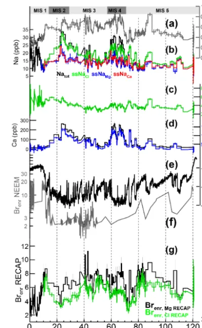
Figure 4.The 120 kyr time series of analyte concentrations in the RECAP ice core. The last 8 kyr are 100-year averages.(a)bromine; (b)total sodium and sea-salt sodium (ssNa) series calculated us-ing chlorine (green), magnesium (blue) and calcium (red);(c) chlo-rine;(d)calcium (black) and magnesium (blue);(e)NGRIPδ18O from North Greenland Ice Core Project members (2004);(f)NEEM Brenrfrom Spolaor et al. (2016b);(g)RECAP Brenrseries (Brenr,Cl, green and Brenr,Mg, black) calculated using chlorine and magne-sium respectively.
index is a semi-quantitative indicator of the local sea ice con-ditions at the marine core location. It is calculated by cou-pling the sediment concentration of IP25, a biomarker
pro-duced by diatoms living in seasonal sea ice, with an open-water phytoplankton biomarker (brassicasterol or dinosterol, hence PBIP25or PDIP25). Briefly, the PIP25index is a
dimen-sionless number varying from 0 to 1: PIP25 ≈ 1 indicates
perennial sea ice cover; PIP25≈0 indicates open-water
con-ditions, while intermediate PIP25values reflect seasonal sea
ice (Müller et al., 2011; Belt and Müller, 2013).
4 Results and discussion
The two Brenr time series (Brenr,Cl and Brenr,Mg), based on
suggesting an FYSI signature throughout the last 120 kyr in the North Atlantic (Fig. 4g). The very low values found in the Holocene (on average Brenr,Hol =3.9, rms (root mean
square)=1.5) suggest minimum FYSI during the current in-terglacial. Although the record does not extend to the Eemian period, it shows that at the inception of the last glacial period, ∼120 000 years ago, Brenr values were higher than in the
Holocene (on average Brenr,120 kyr=5.4, rms=1.1,n=38),
suggesting that more FYSI was present at that time. From 120 kyr ago the Brenrlevels increased until the Greenland
In-terstadial 21 (GI-21),∼85–80 kyr ago (Brenr,85−80 kyr '8).
Hereafter, they decreased throughout late MIS 5. From late MIS 5 to MIS 4, rising Brenrvalues are observed, but a
sta-tistically significant difference between the two Brenrcurves
results from the two ssNa corrections, with the Brenr,Mg
se-ries showing higher values than Brenr,Cl. The two series
con-verge again at the beginning of MIS 3, with values around 7±1. From∼50–40 ka, both series start to decrease. The de-crease is more significant for Brenr,Cl. Minimum Brenrvalues
are reached at the Last Glacial Maximum during MIS 2. The deglaciation reveals a Brenrincrease up to ca. 12 000 years
ago, followed by a steady decrease towards the Holocene. The first Arctic glacial–interglacial investigation of Brenr
was performed on the NEEM ice core, located in northwest Greenland. At NEEM, the main source regions for sea-ice-related processes are believed to the Canadian archipelago, the Baffin Bay and the Hudson Bay (Spolaor et al., 2016b; Schüpbach et al., 2018). The 120 000-year NEEM record (Spolaor et al., 2016b) showed higher Brenr values during
the Holocene and interstadials compared to the glacial stadi-als (Fig. 4f). This was interpreted as greater FYSI conditions existing during such warmer periods, while the lower Brenr
values during colder climate phases would indicate more ex-tended MYSI coverage in those ocean regions. In accordance with their respective source regions, the Brenrrecord from the
NEEM ice core is markedly different from the RECAP one (Fig. 4). In the NEEM core, Brenrwas positively correlated
to δ18O throughout the entire climatic record. In contrast, at Renland, such a consistent correlation is not present, and Brenr is at times lower during warmer climate periods (e.g.
during the Holocene). We suggest that this difference orig-inates from the fact that during warm periods, the relative FYSI-to-OW influence is greater at NEEM than at Renland, the latter being mostly dominated by OW conditions in the North Atlantic. This is supported, at least for present condi-tions, by a model study that investigated the Arctic spatial variability of the ratio of sea ice to open-ocean sodium load-ings (Rhodes et al., 2018), where it was found that such ratio at NEEM is∼5 times higher than Renland.
Since the increase in atmospheric bromine is believed to reflect the strength of bromine recycling from FYSI surfaces, low values of Brenrcould indicate either OW or MYSI
condi-tions. Thus, we suggest that Brenris a signature, at Renland,
of contrasting sea ice states: FYSI/MYSI and FYSI/OW. We also suggest that the former (FYSI/MYSI) occurs
dur-Figure 5.Schematic illustration of marine and (suggested) ice-core-based sea ice indicators as a function of different sea ice con-ditions. Brenr(ice core) and IP25(sediment core) increase as a func-tion of first-year sea ice (FYSI) area. Low values can thus indicate either open-water (OW) or multi-year sea ice (MYSI) conditions, depending on the climate state. The PIP25index is a marine-derived semi-quantitative indicator of local sea ice conditions at the marine core location. PIP25∼0 (PIP25∼1) indicates open-water (peren-nial sea ice, i.e. MYSI) conditions, while intermediate PIP25values reflect seasonal sea ice (i.e. FYSI). Brenrvalues in the RECAP core are believed to indicate an FYSI/OW regime in a “warm” climate state and an FYSI/MYSI in a “cold” climate state.
ing generally colder periods while the latter (FYSI/OW) oc-curs during generally warmer periods. In the framework of this dual regime behaviour, if the ice core time resolution is high enough, an increase in Brenr values followed by a
maximum and a negative trend should be a signature of an ocean facing gradual changes from open ocean to multi-year sea ice conditions, or vice versa, in the case of monotoni-cally warming or cooling ocean temperatures (Fig. 5). One such regime shift is observed in the RECAP Brenrrecord
dur-ing the deglaciation (Fig. 4g). At the Last Glacial Maximum (LGM,∼23 ka), the low enrichment values (Brenr,Mg,LGM
=3.3±0.3; Brenr,Cl,LGM=3.2±0.2) suggest reduced FYSI
recycling and therefore extensive MYSI conditions (blue ar-row in Fig. 5; OW conditions are considered unlikely). Tran-sitioning from the Last Glacial Maximum into the Holocene, Brenr increases until ∼12 ka (Brenr,Mg,12 kyr =8.7±0.9;
Brenr,Cl,12 kyr=7.5±0.5), indicating maximum FYSI at this
time (Figs. 4 and 6). Hereafter, a decrease is observed, as Brenrcontinues to drop during the Early Holocene and the
proxy operates in the FYSI/OW regime (red arrow in Fig. 5).
4.1 The last deglaciation and the dualBrenrregimes We now consider in further detail the last deglaciation, when a number of ocean temperature, salinity, circulation and sea ice changes are observed in the Nordic Seas (Fig. 6). Marine-derived local sea ice records from both the Svalbard mar-gin and the Norwegian Sea indicate (Fig. 6e, f) that near-perennial sea ice (PIP25≈0.5–1) was present during MIS 2
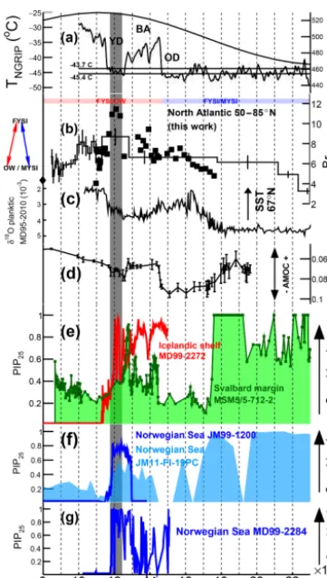
Figure 6.Climate records during the last deglaciation.(a)NGRIP air temperature reconstruction (Kindler et al., 2014) (±1σ= 2.5◦C). The two horizontal lines correspond to a±2σ deviation from the mean temperature (−44.6◦C) found during the 12.4– 11.8 ka period of maximum Brenr,Mg (grey vertical band). The
TNGRIPrecord does not extend before 10 ka but the temperature is not expected to cross the threshold at any time in the Holocene. The black line is the 21 June daily mean insolation at 65◦N (Laskar et al., 2004).(b)RECAP Brenr,Mg(thick black line) and repeat sampling conducted at higher resolution (squares). Since for the highly resolved measurements magnesium was not mea-sured, for the calculation of the sea-salt sodium concentrations and the Brenr,Mg values (Eqs. 1–7) we used the magnesium val-ues of the four low-resolution samples. Over the time period cov-ered by the repeat measurements, nssNa'10 %–20 %. The average Brenr,Mgvalue measured during the Holocene is indicated by a dia-mond.(c)Planktonicδ18O record from sediment core MD95-2010 (66◦41.050N, 04◦33.970E, from Dokken and Jansen, 1999). Lower
δ18O values indicate warmer and fresher ocean waters.(d)Record of231Pa/230Th ratios within a sediment core retrieved in the deep western subtropical Atlantic (33◦420N, 57◦350W). Sedimentary 231Pa/230Th are believed to reflect Atlantic meridional overturn-ing circulation (AMOC) strength (McManus et al., 2004). (e, f, g)PIP25 records from the Svalbard margin (green, core MSM5/5-712-2, Müller and Stein, 2014), the North Icelandic shelf (red, core MD99-2272, Xiao et al., 2017) and the Norwegian Sea (core JM11-FI-19PC from Hoff et al., 2016); core JM99-1200 from Cabedo-Sanz et al. (2013); and core MD99-2284 from Muschitiello et al. (2019). The PIP25 scale varies from perennial sea ice (PIP25≈1) to open-water (PIP25≈0) conditions (see Fig. 5). See Fig. 1 for the PIP25core locations.
Atlantic Ocean are observed (Fig. 6), including seawater surface freshening and warming in the polar and subpolar North Atlantic (the 67◦N Dokken and Jansen, 1999, record is shown as an example in Fig. 6c) and a near total cessation of the Atlantic Meridional Overturning Circulation (AMOC; Fig. 6d). Generally low to intermediate PIP25 values (PIP25
≈0–0.5) are reported in the Svalbard Margin and in the Nor-wegian Sea in the∼17–12 ka period (Fig. 6e, f, g), with a slight increasing trend throughout the Bølling–Allerød (BA) and a broad maximum reached during the Younger Dryas (YD), suggesting that seasonal sea ice conditions were dom-inating this period. Other studies from marine records in the Nordic Seas records also suggest milder sea ice conditions during the BA and increased sea ice during the YD (Belt et al., 2015; Cabedo-Sanz et al., 2016). In contrast, a record from the North Icelandic shelf (Fig. 6e) shows that here the sea ice conditions remained near-perennial from 14.7 to 11.7 ka (PIP25≈0.5–1). The authors (Xiao et al., 2017)
sug-gest that this pattern of more severe sea ice conditions in the north of Iceland is, at least during the BA and the YD, linked to the flow of warmer waters from the North Atlantic Cur-rent, influencing sea ice melting in the eastern Nordic Seas, whereas the Icelandic shelf is influenced by colder polar wa-ters from the East Greenland Current and the East Icelandic Current.
The RECAP ice core was resampled at a sub-centennial resolution to better constrain the timing of sea ice changes through the deglaciation in the 50–85◦N North Atlantic (Fig. 6b, squares). The Brenr,Mgseries (Brenr,Clwould lead to
the same results) would indicate that FYSI started to increase in the North Atlantic, concurrent with a reduction in MYSI, at∼17.5 ka, synchronous with a local PIP25decrease in the
Svalbard margin and eastern Nordic Seas and in response to sea surface temperature warming in the North Atlantic. This finding would also suggest that North Atlantic sea ice changes occurred in concert with temperature and circula-tion changes in the underlying surface waters. We note that this time period also coincides with the initiation of deglacial changes in mean ocean temperature, Antarctic temperatures and atmospheric CO2concentrations toward interglacial
val-ues (Bereiter et al., 2018). North Atlantic FYSI continued to increase throughout the BA (except for one point at 12.7– 12.4 ka at the onset of the YD) until a maximum at 12.4– 11.8 ka during the YD, when a clear Brenr,Mg maximum is
observed (Fig. 6b). From the comparison between the marine and ice core results, we infer that, during the 17–12 ka period, the 50–85◦N-integrated North Atlantic sea ice changed from MYSI to FYSI. Local sea ice was also melting at∼17 ka in the eastern Nordic Seas, likely influenced by the North At-lantic Current, while, at least from 14.7 to 11.7 ka, sea ice was still near-perennial at the North Icelandic shelf, possibly due to the influence of cold waters carried by the East Green-land Current. Following its maximum value at 12.4–11.8 ka, Brenr (i.e. FYSI) started to decrease (Fig. 6b). We suggest
the FYSI/OW regime (Fig. 5), and the North Atlantic basin becomes largely ice free. A retreating FYSI scenario is also recorded in all five marine cores (decreasing PIP25 to≈0–
0.4 during the Early Holocene; Fig. 6e, f, g), suggesting that open-water conditions progressively developed in the whole North Atlantic basin, sustained by increasing heat transport from the North Atlantic Current and a strengthened AMOC since∼11.7 ka (McManus et al., 2004; Ritz et al., 2013).
Since Brenr is assumed to be an increasing function of
FYSI, its decrease would point to either OW or MYSI con-ditions, following either the FYSI/OW or the FYSI/MYSI regimes (Fig. 5). At any point in time, only one regime is considered to be in place, and we suggest a simple model in which a temperature threshold could be the discriminating variable setting the regime type. Since a change in regime is observed during the deglaciation, with maximum Brenr
val-ues (i.e. FYSI) at 11.8–12.4 ka, we set the threshold to be the mean NGRIP ice core temperature reconstructed for that pe-riod: TNGRIP= −44.6±0.9 (2σ)◦C (the two lines in Fig. 6a).
In every ice sample of the 120 000-year record the regime type (FYSI/MYSI or FYSI/OW; Fig. 5) can thus be deter-mined according to its integrated temperature value with re-spect to the temperature threshold: FYSI/MYSI for a lower temperature value and FYSI/OW for a higher temperature value.
According to this simple model the deglaciation is char-acterized by the FYSI/MYSI regime until the onset of the Bølling–Allerød (except few points at which the regime type depends on the chosen threshold value; Sect. 4.2), while the FYSI/OW regime operated from that point forward. We note that there is no similar Brenrmaximum at the onset of the
Bølling–Allerød as seen in the YD at the point when NGRIP temperature is crossing the same temperature as found in the YD. The possible explanation of higher Brenrvalues during
the Younger Dryas compared to the Bølling–Allerød may re-side in the higher seasonal temperature variations (Buizert et al., 2014) and freshwater inputs from melting ice sheets in the former period, both promoting the formation of seasonal sea ice. Conversely, the lower Brenrvalues (hence to greater
MYSI in the FYSI/MYSI regime) during the Older Dryas compared to the Bølling–Allerød and the Younger Dryas may be linked to the overall much lower temperatures during this period (Buizert et al., 2014), higher surface water salinity due to less freshwater inputs from melting ice sheets and a generally weaker AMOC. It appears that the NGRIP tem-perature threshold alone is unable to fully represent the sug-gested two-regime modelization during the deglaciation, pos-sibly due to concomitant changes in other sea-ice-related cli-mate variables during this period. We suggest that at glacial– interglacial timescales such a temperature-based discrimina-tion could be still used to represent the two-regime variabil-ity.
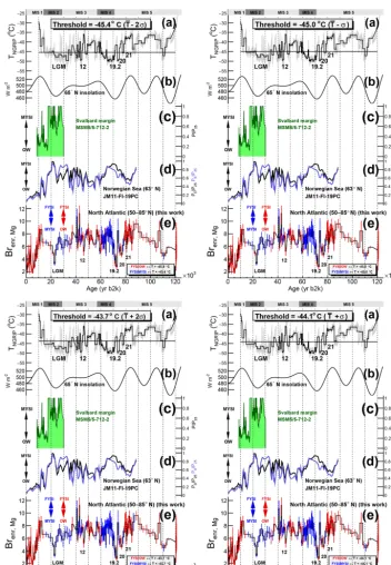
Figure 7.Discrimination between the two Brenr,Mg regimes ac-cording to the−44.6◦C NGRIP temperature threshold and North Atlantic sea ice records from marine cores. (a) Reconstructed NGRIP temperature (grey; Kindler et al., 2014). The temperature threshold value is the mean temperature during the 11.8–12.4 ka pe-riod, when the change in Brenr,Mgregime was observed (see Fig. 6). The black series is the NGRIP temperature profile downscaled to the measured Brenrresolution. The numbers indicate the Greenland Interstadials (GIs) discussed in the text.(b)Daily mean insolation on 21 June at 65◦N (Laskar et al., 2004).(c)PIP25 record from the Svalbard margin (core MSM5/5-712-2 from Müller and Stein, 2014).(d)PDIP25and PBIP2590 kyr records from the Norwegian Sea presented as five-point running mean (from Hoff et al., 2016). (e)Discrimination between the Brenr,Mgregimes computed accord-ing to the integrated temperature value with respect to the threshold. The FYSI/OW and FYSI/MYSI regimes are indicated with red and blue error bars respectively.
4.2 The 120 000-yearBrenrrecord
We now apply the previously mentioned temperature-based discrimination between the two sea ice regimes to the 120 000-year Brenr,Mg record (Fig. 7). The regime type in
-2(1)σ scenario during the deglaciation (Fig. D1), the regime discrimination mentioned in the following discussion is in-variant with respect to the four temperature-based scenarios. The same analysis is also performed on the Brenr,Cl curves
(Fig. D2).
MIS 5 is characterized by increasing Brenr,Mgvalues in the
FYSI/OW regime from 120 to 80 kyr ago (Greenland Inter-stadial, GI-21, Fig. 7). We interpret this trend with increas-ing FYSI extent in the North Atlantic. From the end of GI-21 the Brenrregime changes to FYSI/MYSI as the NGRIP
tem-perature drops during late MIS 5 and MIS 4. As compared to the levels reached during GI-21 (8±1), lower Brenr,Mg
values are found during GS-21, GS-20 and GS-19 (5±2) and on average during MIS 4 (7±1). We interpret the com-bined effect of decreased Brenr,Mgvalues in the FYSI/MYSI
regime with an increase in MYSI extent in the North Atlantic from late MIS 5 to MIS 4. The Brenr,Cl curve shows even
lower values during MIS 4, predicting more extended MYSI than the Brenr,Mg record (Fig. D2). Overall, from 120 kyr
ago to MIS 4, the change in Brenrregime (from FYSI/OW
to FYSI/MYSI) is opposite to what is observed during the deglaciation (from FYSI/MYSI to FYSI/OW): from a rela-tively warm climate 120 kyr ago, the cooling trend is char-acterized by an increasing FYSI extent until the point (GI-21) at which the FYSI starts to be replaced by MYSI. This maximum Brenr,Mg value at the time of the regime change
(GI-21) is similar to the peak Brenr,Mg value reached
dur-ing the deglaciation: Brenr,Mg(12 kyr)'Brenr,Mg(GI-21)'8.
The same result holds if one considers the Brenr,Cl series
(Fig. D2). Unlike the longer lasting GI-21, the Greenland In-terstadials GI-20 and GI-19.2 display very low Brenrvalues
('3–5). A possible explanation for these low values could be found in a fast replacement (at least not captured by the time resolution of the Brenrrecord) of MYSI by OW
condi-tions. Higher time-resolved measurements would be needed to test this hypothesis.
Moving from MIS 4 to MIS 3, the Brenr,Mgvalues remain
within 1σ of each other. This suggests a similar FYSI extent in the two periods, although the FYSI/MYSI regime operat-ing duroperat-ing MIS 4 could suggest an extra MYSI extent duroperat-ing this period, as compared to MIS 3, the latter being gener-ally characterized by a mixture of both Brenr regimes. This
hypothesis is supported by the Brenr,Cl series, which shows
lower values during MIS 4 than MIS 3 (Fig. D2). A sea ice record in the Norwegian Sea (Hoff et al., 2016) also indicates more perennial sea ice conditions during MIS 4 than during MIS 3. The time resolution does not allow a deep investiga-tion of DO events during MIS 3, although a low Brenrvalue
in the FYSI/OW regime during the GI-12 (Brenr,Mg(46.0–
46.6 ka) =5.2±0.7) suggests a shift to open-water condi-tions during this interstadial, similarly to GI-19.2 and GI-20. Possibly, similar sea ice dynamics were in play during these stadial–interstadial transitions. Increased time resolution is, however, needed to better characterize DO events.
MIS 2 is characterized by an FYSI/MYSI regime and pro-gressively decreasing Brenr,Mgvalues (Fig. 7e), with a
min-imum being reached∼23 kyr ago, during the Last Glacial Maximum: Brenr,Mg(LGM) =3.3±0.3. We interpret this
negative Brenr,Mg(and Brenr,Cl, Fig. D2) trend with
progres-sively increasing MYSI conditions in the whole North At-lantic, which reached a maximum during the LGM. Rela-tively high and increasing PIP25values (≈0.5–1) are found
in the Norwegian Sea record (Fig. 7d), with maximum sea ice registered ca. 20–23 kyr ago. The sea ice record from Fram Strait is in broad agreement with the Norwegian record, the former showing high (≈0.5–1) and variable PIP25values
un-til the longer lasting 19 ka maximum (Fig. 7c). Overall, the cold MIS 2 period is characterized by decreasing seasonal sea ice and increasing multi-year sea ice across the North Atlantic, with a maximum reached ca. 20 kyr ago.
The deglaciation is characterized by increasing FYSI con-ditions until the mid-Younger Dryas (12.4–11.8 kyr ago), fol-lowed by a return to the FYSI/OW regime and decreasing Brenr values as open waters progressively replaced sea ice
in the Holocene. A clear sea ice decline is also reported in the Norwegian Sea following the LGM towards the current interglacial (Figs. 6 and 7).
5 Conclusions and outlook
We present a 120 000-year record of bromine enrichment (Brenr) from the RECAP ice core and interpret it in terms of
These analyses and conclusions rely on a number of hy-potheses and assumptions mainly concerning the validity of Brenras a proxy for first-year sea ice. Efforts are still needed
in the direction of validating these assumption and investi-gating the limitations and processes that affect the Brenr
sig-nature in present deposition and in old ice core records.
Appendix A: Bromine loss from the snowpack
The stability of bromine after deposition has been questioned since the first investigation carried out by Dibb et al. (2010) in Summit (Greenland). We summarize here the experimen-tal investigations that have been carried out on this topic ever since both in Antarctica and in the Arctic.
A1 Antarctica
McConnell et al. (2017) investigated simultaneous sodium and bromine fluxes across Antarctica (see their Fig. S4 in the Appendix showing the reconstructed fluxes from an array of 11 cores measured in McConnell et al., 2014). In particular, theJ(Na) andJ(Br)–accumulation rate (A) linear relations (impressiveJ(Br)–Alinear fit from 50 to 400 kg m−2yr−1) suggest that, while sodium loss is negligible, bromine re-emission is quantified to 17±2 µg m−2yr−1 (negative
in-tercept, i.e. snow–air flux). According to the results, the bromine loss from Antarctic snowpack would be 65 % at sites with A=50 kg m−2yr−1, 32 % at sites with A= 100 kg m−2yr−1, 22 % at sites with A=150 kg m−2yr−1, 16 % at sites with A=200 kg m−2yr−1, 13 % at sites with A=250 kg m−2yr−1 and 11 % at sites with A= 300 kg m−2yr−1(note that this exercise works on the hypoth-esis that the bromine air concentration is the same above all sites, but the goodness of their fit would suggest that this is the case). These negative fluxes would be representative of Antarctic conditions for the duration of the records, i.e. few centuries to 2 millennia maximum (see Supplement Table S2 in the 2014 ref). In their Dome C (A=30 kg m−2yr−1) study, Legrand et al. (2016) analysed bromine content in a 110 cm deep, 2 cm resolution snow pit. Their measurements show that the upper 2 cm contain 1.25 times more bromine that the 2–4 cm layer, 2.5 times more than the 4–8 cm layer and ca. 10 times more than the 8–12 cm layer. Based on the higher bromine concentrations towards the surface the au-thors suggest a possible bromine remobilization from the snow. In testing the hypothesis, the authors model whether the measured bromine snow content is high enough to sus-tain the 1.7 pptv air concentration of Brythey measured in the
overlying atmosphere. They find that to explain such a value, the snow bromine storage should be 35 times larger than the actual measurements. They therefore conclude that in Dome C their investigation do not support the importance of snow-pack bromine emissions. This conclusion contrasts with what would be concluded by McConnell and co-workers.
From a surface snow experiments carried out in Dome C in 2014 (Antarctica,A=30 kg m−2yr−1) by Spolaor et al. (2018), the authors observe constant bromine concentrations from mid-December to mid-January (austral summer). In a similar experiment carried out the following year, from late November to late December 2015, higher bromine concen-trations were found in November (late spring) with a de-creasing trend towards the end of the year. The authors relate
such a drop to a change in the source of the air masses, from coastal to inland, as inferred from back trajectory modelling, rather than to bromine loss from the snow.
From another surface snow experiment carried out at GV7 (Antarctica,A=270 kg m−2yr−1), Vallelonga et al. (QSR, 2019) compare bromine fresh surface snow concentrations with snow pit values and suggest, on the basis of similar values between the values in the surface samples and in the surface of the snow pit (that would integrate the values of the surface samples), that at this site bromine is stable af-ter deposition (the McConnell calculation would predict a loss of 12 %). Looking at the 100–300 µg m−2yr−1 annual bromine (2010, 2011, 2012, 2013) fluxes calculated along the Talos Dome–GV7 traverse (Maffezzoli et al., 2017), a nega-tive flux of 17±2 µg m−2yr−1would imply that, if present, the bromine loss can be quantified in this region as 6 %– 17 %. As McConnell and co-workers point out, it is surpris-ing that the snow–air bromine flux they found is not depen-dent on snow accumulation (their fit appears linear until the last point: 400 kg m−2yr−1).
A2 Arctic
In the Arctic, the most robust piece of evidence results from hourly resolved surface snow measurements carried out in coastal Svalbard, showing that bromine photolytic loss can-not be appreciated across night–day cycles (Spolaor et al., 2019; see Fig. 6).
In an experiment described in QSR (2019) that Valle-longa and co-workers carried out in Ny-Ålesund (Svalbard, A=600 kg m−2yr−1), sodium and bromine were measured in surface snow daily from April to June (spring to summer). From April to late May Brenr values decreased by a factor
of 2 (max) (afterwards surface melting and positive temper-atures led to 80 % sodium drainage from the snowpack). It is difficult, however, to determine whether this decrease is due to bromine re-emission or to early spring bromine explosions from sea ice surfaces, located ca. 150 km away from the sam-pling site, enriching the spring deposited snow layers.
A3 Conclusive remarks on bromine loss
re-Table A1.Compilation Na/Mg, Na/Ca and Ca/Mg mass ratios in dust samples originating from north Asia deserts.
Ta et al. (2003) Results of the X-ray fluorescence analysis of soil samples from the desert/Gobi areas in Gansu province, China
Desert areas Gobi areas
– Dunhuang Yumen Anxi Zhangye Linze Wuwei Gulang Yumen Anxi
Na2O (% ox) 1.97 2.05 1.19 1.46 1.76 1.59 1.47 1.36 2.62
MgO (% ox) 1.96 2 3 1.42 1.38 1.05 0.91 1.16 1.3
CaO (% ox) 6.5 6.31 10.59 2.21 2.95 2.23 2.23 8.4 4.88
Na (ppm) 14615 15208 8828 10831 13057 11796 10905 10089 19437
Mg (ppm) 11821 12062 18093 8564 8323 6333 5488 6996 7840
Ca (ppm) 46456 45098 75687 15795 21084 15938 15938 60035 34877
Na/Mg 1.24 1.26 0.49 1.26 1.57 1.86 1.99 1.44 2.48
Na/Ca 0.31 0.34 0.12 0.69 0.62 0.74 0.68 0.17 0.56
Ca/Mg 3.93 3.74 4.18 1.84 2.53 2.52 2.90 8.58 4.45
Wang et al. (2018) Results of total suspended particle elemental concentrations in samples collected at Fudan University (Shanghai, China) during the 19 to 22 March 2010 dust storm estimated to originate from the Gobi Desert.
– 19 Night 20 Day 20 Night 21 Day 21 Night
Na (µg m−3) 1.3 7.9 19.1 2.8 3.9
Mg (µg m−3) 1.4 9.5 14.4 2.2 2.3
Ca (µg m−3) 8.5 37.3 56.9 9.4 8.6
Na/Mg 0.93 0.83 1.33 1.27 1.70
Na/Ca 0.15 0.21 0.34 0.30 0.45
Ca/Mg 6.07 3.93 3.95 4.27 3.74
Sun et al. (2005) Elemental concentrations in aerosols sampled during two springtime 2002 desert storms that hit Beijing, both of which originated from north Asia deserts.
– Desert storm 1 Desert storm 2
Na (µg m−3) 37 39
Mg (µg m−3) 34 29
Ca (µg m−3) 178 58
Na/Mg 1.09 1.34
Na/Ca 0.21 0.67
Ca/Mg 5.24 2.00
Fan et al. (2013) Elemental concentrations measured in Guangzhou (China) during the 23–25 April 2009 dust storm originating in North China.
– Desert storm
Na (µg m−3) 2.98
Mg (µg m−3) 2.83
Ca (µg m−3) 5.78
Na/Mg 1.05
Na/Ca 0.52
Ca/Mg 2.04
Zhang et al. (2002) Composition of air-volume-based concentration of aerosols sampled in Minquin (northwest China desert region) in March–May 1995 and April–June 1996.
– Minquin 1995 Minquin 1996
– Geometric mean Average Geometric mean Average
Na (µg m−3) 1.37 3.22 1.24 1.8
Mg (µg m−3) 2.14 4.4 2.07 2.88
Ca (µg m−3) 5.7 11.4 6.21 8.41
Na/Mg 0.64 0.73 0.60 0.63
Na/Ca 0.24 0.28 0.20 0.21
Ca/Mg 2.66 2.59 3.00 2.92
Wang et al. (2009) Arithmetic mean elemental concentrations measured inn=317 dust fallout samples collected from 33 sites located in the Gobi Desert, sandy desert, loess, and steppes in North China from April 2001 to March 2002.
Na (%) 1.47
Mg (%) 1.01
Ca (%) 3.40
Na/Mg 1.46
Na/Ca 0.43
gardless of snow accumulation, while at GV7 bromine loss was not detected (Vallelonga et al., QSR, 2019). In the Arc-tic, photolytic loss was not detected in Svalbard. Other ex-periments have been shown to be inconclusive due to the presence of surface melting. At sites like Renland (where Holocene melting occurs; see Taranczewski et al., 2019), the extremely high snow accumulation could in general suggest a reduced bromine loss, but again, the 5-fold decrease in snow accumulation during the glacial (preliminaryAglacial,stadials=
100 kg m−2yr−1(Bo M. Vinther, unpublished data)) may in-troduce a possible bromine loss during periods of reduced accumulation, thus increasing Brenrvalues during the coldest
parts of the record. To test these hypotheses and especially the bromine loss during the glacial, a surface study should be carried out at a 100 kg m−2yr−1accumulation site in Green-land. To conclude, at present there are not enough data avail-able to quantify the possible bromine loss from the Renland ice cap, but if present, and depending on accumulation, the effect would be to increase the measured Brenrvalues during
the coldest sections of the glacial period.
Appendix B: ModernNa/MgandNa/Caratios in dust from northern Asian deserts
The aim of this section is to obtain a reference value for the present-day mass ratios of Na/Mg and Na/Ca in Asian dust, since the Gobi and desert regions of Mongolian and northern China (hereafter referred to as Asian dust) are believed to be the main source regions of dust found in Greenlandic ice cores during the glacial period, as inferred from Sr, Nd and Pb isotope composition (Biscaye et al., 1997).
We considern=6 published studies in which the chem-ical composition of dust sampled during “desert events” (DSs) was analysed in China. Often these studies are car-ried out in the framework of pollution-related research. We also include composition data from dust sampled in situ in desert areas. For details on the single studies, we refer the reader to the references in Table A1. We note that our com-pilation only considers dust samples originating (or sampled directly) from deserts. Other geochemical data from such ref-erences that considered trajectories that travelled over other areas (marine or others), are not considered.
By considering all the above-mentioned studies, the mean Na/Mg mass ratio is 1.23 (median=1.26). The mean Na/Ca mass ratio is 0.38 (median=0.33). The mean Ca/Mg mass ratio is 3.66 (median=3.55).
Appendix C: Bromine–sodium correlation in the RECAP ice core
Appendix D: Sensitivity of theBrenr,Mg andBrenr,Cl
regimes to the NGRIP temperature threshold
Author contributions. PV and AS conceived the experiment. NM, RE, PV, AS, HAK and CT collected the samples and ran the experimental analyses. NM analysed and interpreted the results. NM wrote the paper with inputs from all authors.
Competing interests. The authors declare that they have no con-flict of interest.
Acknowledgements. We thank the whole Continuous Flow
Analysis team at the Centre for Ice and Climate (Copenhagen, Denmark) for the sample collection. We thank Trevor Popp, Stef-fen Bo Hansen and the RECAP drilling group and Joel Pedro, Markus Jochum and Trond Dokken for the fruitful discussions. We thank the five reviewers for their constructive comments to im-prove the paper. We thank Zhao Meixun and Francesco Muschi-tiello for sharing the Icelandic and Norwegian core data. We thank Giovanni Baccolo for his useful insights.
Financial support. The RECAP ice coring effort was financed by the Danish Research Council through a Sapere Aude Grant, the NSF through the Division of Polar Programs, the Alfred We-gener Institute, and the European Research Council under the Eu-ropean Community’s Seventh Framework Programme (FP7/2007-2013)/ERC grant agreement 610055 through the Ice2Ice project and the Early Human Impact project (grant agreement 267696). This study has also received funding from the European Research Council Executive Agency under the European Union’s Horizon 2020 Research and Innovation programme (Project ERC-2016-COG 726349 CLIMAHAL).
Review statement. This paper was edited by Amaelle Landais and reviewed by five anonymous referees.
References
Abbatt, J.: Arctic snowpack bromine release, Nat. Geosci., 6, 331– 332, https://doi.org/10.1038/ngeo1805, 2013.
Abbatt, J. P. D., Thomas, J. L., Abrahamsson, K., Boxe, C., Gran-fors, A., Jones, A. E., King, M. D., Saiz-Lopez, A., Shep-son, P. B., Sodeau, J., Toohey, D. W., Toubin, C., von Glasow, R., Wren, S. N., and Yang, X.: Halogen activation via interac-tions with environmental ice and snow in the polar lower tropo-sphere and other regions, Atmos. Chem. Phys., 12, 6237–6271, https://doi.org/10.5194/acp-12-6237-2012, 2012.
Ashbaugh, L. L., Malm, W. C., and Sadeh, W. Z.: A residence time probability analysis of sulfur concentrations at Grand Canyon National Park, Atmos. Environ., 19, 1263–1270, 1985.
Barrie, L., Bottenheim, J., Schnell, R., Crutzen, P., and Rasmussen, R.: Ozone destruction and photochemical reactions at polar sun-rise in the lower Arctic atmosphere, Nature, 334, 138–141, 1988. Belt, S. T. and Müller, J.: The Arctic sea ice biomarker IP 25: a review of current understanding, recommendations for future re-search and applications in palaeo sea ice reconstructions, Quater-nary Sci. Rev., 79, 9–25, 2013.
Belt, S. T., Cabedo-Sanz, P., Smik, L., Navarro-Rodriguez, A., Berben, S. M., Knies, J., and Husum, K.: Identification of pa-leo Arctic winter sea ice limits and the marginal ice zone: opti-mised biomarker-based reconstructions of late Quaternary Arctic sea ice, Earth Planet. Sc. Lett., 431, 127–139, 2015.
Bereiter, B., Shackleton, S., Baggenstos, D., Kawamura, K., and Severinghaus, J.: Mean global ocean tempera-tures during the last glacial transition, Nature, 553, 39–44, https://doi.org/10.1038/nature25152, 2018.
Bigler, M., Svensson, A., Kettner, E., Vallelonga, P., Nielsen, M. E., and Steffensen, J. P.: Optimization of high-resolution continuous flow analysis for transient climate signals in ice cores, Environ. Sci. Technol., 45, 4483–4489, 2011.
Biscaye, P., Grousset, F., Revel, M., Van der Gaast, S., Zielinski, G., Vaars, A., and Kukla, G.: Asian provenance of glacial dust (stage 2) in the Greenland Ice Sheet Project 2 ice core, Summit, Greenland, J. Geophys. Res.-Oceans, 102, 26765–26781, 1997. Buizert, C., Gkinis, V., Severinghaus, J. P., He, F., Lecavalier,
B. S., Kindler, P., Leuenberger, M., Carlson, A. E., Vinther, B., Masson-Delmotte, V., White, J. W., Liu, Z., Otto-Bliesner, B., Brook, E. J.: Greenland temperature response to climate forcing during the last deglaciation, Science, 345, 1177–1180, https://doi.org/10.1126/science.1254961, 2014.
Cabedo-Sanz, P., Belt, S. T., Knies, J., and Husum, K.: Identification of contrasting seasonal sea ice conditions during the Younger Dryas, Quaternary Sci. Rev., 79, 74–86, 2013.
Cabedo-Sanz, P., Belt, S. T., Jennings, A. E., Andrews, J. T., and Geirsdóttir, Á.: Variability in drift ice export from the Arctic Ocean to the North Icelandic Shelf over the last 8000 years: a multi-proxy evaluation, Quaternary Sci. Rev., 146, 99–115, 2016.
Chance, K.: Analysis of BrO measurements from the global ozone monitoring experiment, Geophys. Res. Lett., 25, 3335–3338, 1998.
Corella, J. P., Maffezzoli, N., Cuevas, C. A., Vallelonga, P., Spo-laor, A., Cozzi, G., Müller, J., Vinther, B., Barbante, C., Kjaer, H. A., Edwards, R., and Saiz-Lopez, A.: Holocene atmospheric iodine evolution over the North Atlantic, Clim. Past Discuss., https://doi.org/10.5194/cp-2019-71, in review, 2019.
Cuevas, C. A., Maffezzoli, N., Corella, J. P., Spolaor, A., Vallelonga, P., Kjær, H. A., Simonsen, M., Winstrup, M., Vinther, B., Horvat, C., Fernandez, R. P., Kinnison, D. E., Lamarque, J., Barbante, C., and Saiz-Lopez, A.: Rapid increase in atmospheric iodine levels in the North Atlantic since the mid-20th century, Nat. Commun., 9, 1452, https://doi.org/10.1038/s41467-018-03756-1, 2018. De Angelis, M., Steffensen, J. P., Legrand, M., Clausen, H., and
Hammer, C.: Primary aerosol (sea salt and soil dust) deposited in Greenland ice during the last climatic cycle: Comparison with east Antarctic records, J. Geophys. Res.-Oceans, 102, 26681– 26698, 1997.
Dibb, J. E., Ziemba, L. D., Luxford, J., and Beckman, P.: Bromide and other ions in the snow, firn air, and atmospheric boundary layer at Summit during GSHOX, Atmos. Chem. Phys., 10, 9931– 9942, https://doi.org/10.5194/acp-10-9931-2010, 2010. Dokken, T. M. and Jansen, E.: Rapid changes in the mechanism
Draxler, R. and Hess, G.: Description of the HYSPLIT 4 model-ing system NOAA Tech, NOAA Tech Memo ERL ARL-224, 24, 1997.
Draxler, R. R. and Hess, G.: An overview of the HYSPLIT_4 mod-elling system for trajectories, Aust. Meteorol. Mag., 47, 295– 308, 1998.
Draxler, R. R., Stunder, B., Rolph, G., and Taylor, A.: HYSPLIT4 Users’s Guide, US Department of Commerce, National Oceanic and Atmospheric Administration, Environmental Research Lab-oratories, Air Resources Laboratory, 1999.
Fan, Q., Shen, C., Wang, X., Li, Y., Huang, W., Liang, G., Wang, S., and Huang, Z.: Impact of a dust storm on characteristics of particle matter (PM) in Guangzhou, China, Asia-Pac. J. Atmos. Sci., 49, 121–131, 2013.
Frey, M. M., Norris, S. J., Brooks, I. M., Anderson, P. S., Nishimura, K., Yang, X., Jones, A. E., Nerentorp Mastromonaco, M. G., Jones, D. H., and Wolff, E. W.: First direct observation of sea salt aerosol production from blowing snow above sea ice, Atmos. Chem. Phys. Discuss., https://doi.org/10.5194/acp-2019-259, in review, 2019.
Hansson, M. E.: The Renland ice core. A Northern Hemi-sphere record of aerosol composition over 120,000 years, Tellus B, 46, 390–418, https://doi.org/10.1034/j.1600-0889.1994.t01-4-00005.x, 1994.
Hoff, U., Rasmussen, T. L., Stein, R., Ezat, M. M., and Fahl, K.: Sea ice and millennial-scale climate variability in the Nordic seas 90 [thinsp] kyr ago to present, Nat. Commun., 7, 12247, https://doi.org/10.1038/ncomms12247, 2016.
Kalnay, E., Kanamitsu, M., Kistler, R., Collins, W., Deaven, D., Gandin, L., Iredell, M., Saha, S., White, G., Woollen, J., Zhu, Y., Chelliah, M., Ebisuzaki, W., Higgins, W., Janowiak, J., Mo, K. C., Ropelewski, C., Wang, J., Leetmaa, A., Reynolds, R., Jenne, R., and Joseph, D.: The NCEP/NCAR 40-year reanalysis project, B. Am. Meteorol. Soc., 77, 437–471, 1996.
Kaufmann, P. R., Federer, U., Hutterli, M. A., Bigler, M., Schüp-bach, S., Ruth, U., Schmitt, J., and Stocker, T. F.: An improved continuous flow analysis system for high-resolution field mea-surements on ice cores, Environ. Sci. Technol., 42, 8044–8050, 2008.
Kindler, P., Guillevic, M., Baumgartner, M., Schwander, J., Landais, A., and Leuenberger, M.: Temperature reconstruction from 10 to 120 kyr b2k from the NGRIP ice core, Clim. Past, 10, 887–902, https://doi.org/10.5194/cp-10-887-2014, 2014.
Kreher, K., Johnston, P., Wood, S., Nardi, B., and Platt, U.: Ground-based measurements of tropospheric and stratospheric BrO at Ar-rival Heights, Antarctica, Geophys. Res. Lett., 24, 3021–3024, 1997.
Laskar, J., Robutel, P., Joutel, F., Gastineau, M., Correia, A., and Levrard, B.: A long-term numerical solution for the insolation quantities of the Earth, Astron. Astrophys., 428, 261–285, 2004. Legrand, M. and Mayewski, P.: Glaciochemistry of polar ice cores:
a review, Rev. Geophys., 35, 219–243, 1997.
Legrand, M., Yang, X., Preunkert, S., and Theys, N.: Year-round records of sea salt, gaseous, and particulate inorganic bromine in the atmospheric boundary layer at coastal (Dumont d’Urville) and central (Concordia) East Antarctic sites, J. Geophys. Res.-Atmos., 121, 997–1023, 2016.
Legrand, M. R. and Delmas, R. J.: Formation of HCl in the Antarctic atmosphere, J. Geophys. Res.-Atmos., 93, 7153–7168, 1988.
Lewis, E. R. and Schwartz, S. E.: Sea salt aerosol production: mech-anisms, methods, measurements, and models – A critical review, vol. 152, American Geophysical Union, 2004.
Li, C., Kang, S., Shi, G., Huang, J., Ding, M., Zhang, Q., Zhang, L., Guo, J., Xiao, C., Hou, S., Sun, B., Qin, D., and Ren, R.: Spatial and temporal variations of total mercury in Antarctic snow along the transect from Zhongshan Station to Dome A, Tellus B, 66, 25152, https://doi.org/10.3402/tellusb.v66.25152, 2014. Maffezzoli, N., Spolaor, A., Barbante, C., Bertò, M., Frezzotti,
M., and Vallelonga, P.: Bromine, iodine and sodium in sur-face snow along the 2013 Talos Dome–GV7 traverse (northern Victoria Land, East Antarctica), The Cryosphere, 11, 693–705, https://doi.org/10.5194/tc-11-693-2017, 2017.
Maggi, V.: Mineralogy of atmospheric microparticles deposited along the Greenland Ice Core Project ice core, J. Geophys. Res.-Oceans, 102, 26725–26734, 1997.
Mayewski, P. A., Meeker, L. D., Whitlow, S., Twickler, M. S., Mor-rison, M. C., Bloomfield, P., Bond, G., Alley, R. B., Gow, A. J., Meese, D. A., Ram M., Taylor, K. C., and Wumkes, W.: Changes in atmospheric circulation and ocean ice cover over the North Atlantic during the last 41 000 years, Science, 263, 1747–1751, 1994.
McConnell, J. R., Maselli, O. J., Sigl, M., Vallelonga, P., Neu-mann, T., Anschütz, H., Bales, R. C., Curran, M. A., Das, S. B., Edwards, R., Kipfstuhl, S., Layman, L., and Thomas, E. R.: Antarctic-wide array of high-resolution ice core records reveals pervasive lead pollution began in 1889 and persists today, Sci. Rep., 4, 5848, https://doi.org/0.1038/srep05848, 2014.
McConnell, J. R., Burke, A., Dunbar, N. W., Köhler, P., Thomas, J. L., Arienzo, M. M., Chellman, N. J., Maselli, O. J., Sigl, M., Adkins, J. F., Baggenstos, D., Burkhart, J. F. , Brook, E. J., Buizert, C., Cole-Dai, J., Fudge, T. J., Knorr, G., Graf, H.-F., Grieman, M. M., Iverson, N., McGwire, K. C., Mulvaney, R., Paris, G., Rhodes, R. H., Saltzman, E. S., Severinghaus, J. P., Steffensen, J. P., Taylor, K. C., and Winckler, G.: Synchronous volcanic eruptions and abrupt climate change 17.7 ka plausibly linked by stratospheric ozone depletion, P. Natl. Acad. Sci. USA, 114, 10035–10040, 2017.
McManus, J. F., Francois, R., Gherardi, J.-M., Keigwin, L. D., and Brown-Leger, S.: Collapse and rapid resumption of Atlantic meridional circulation linked to deglacial climate changes, Na-ture, 428, 834–837, https://doi.org/10.1038/nature02494, 2004. Millero, F. J., Feistel, R., Wright, D. G., and McDougall, T. J.:
The composition of Standard Seawater and the definition of the Reference-Composition Salinity Scale, Deep Sea-Res. Pt. I, 55, 50–72, https://doi.org/10.1016/j.dsr.2007.10.001, 2008. Müller, J. and Stein, R.: High-resolution record of late glacial and
deglacial sea ice changes in Fram Strait corroborates ice–ocean interactions during abrupt climate shifts, Earth Planet. Sc. Lett., 403, 446–455, 2014.