modern plausible parameter sets
Krista M. S. Kemppinen1, Philip B. Holden2, Neil R. Edwards2, Andy Ridgwell3,4, and Andrew D. Friend1 1Department of Geography, University of Cambridge, Cambridge, CB2 3EN, UK
2Environment, Earth and Ecosystem Sciences, The Open University, Milton Keynes, MK7 6AA, UK
3School of Geographical Sciences, Bristol University, Bristol, BS8 1SS, UK
4Department of Earth Sciences, University of California, Riverside, CA 92521, USA
Correspondence:Krista M. S. Kemppinen ([email protected]) Received: 17 December 2017 – Discussion started: 5 January 2018 Revised: 8 May 2019 – Accepted: 10 May 2019 – Published: 18 June 2019
Abstract.During the Last Glacial Maximum (LGM), atmo-spheric CO2was around 90 ppmv lower than during the pre-industrial period. The reasons for this decrease are most often elucidated through factorial experiments testing the impact of individual mechanisms. Due to uncertainty in our under-standing of the real system, however, the different models used to conduct the experiments inevitably take on different parameter values and different structures. In this paper, the objective is therefore to take an uncertainty-based approach to investigating the LGM CO2 drop by simulating it with a large ensemble of parameter sets, designed to allow for a wide range of large-scale feedback response strengths. Our aim is not to definitely explain the causes of the CO2drop but rather explore the range of possible responses. We find that the LGM CO2decrease tends to predominantly be associated with decreasing sea surface temperatures (SSTs), increasing sea ice area, a weakening of the Atlantic Meridional Over-turning Circulation (AMOC), a strengthening of the Antarc-tic Bottom Water (AABW) cell in the AtlanAntarc-tic Ocean, a de-creasing ocean biological productivity, an inde-creasing CaCO3 weathering flux and an increasing deep-sea CaCO3 burial flux. The majority of our simulations also predict an increase in terrestrial carbon, coupled with a decrease in ocean and in-crease in lithospheric carbon. We attribute the inin-crease in ter-restrial carbon to a slower soil respiration rate, as well as the preservation rather than destruction of carbon by the LGM ice sheets. An initial comparison of these dominant changes with observations and paleoproxies other than carbon isotope and oxygen data (not evaluated directly in this study)
sug-gests broad agreement. However, we advise more detailed comparisons in the future, and also note that, conceptually at least, our results can only be reconciled with carbon isotope and oxygen data if additional processes not included in our model are brought into play.
1 Introduction
rejec-tion (Shin et al., 2003; Bouttes et al., 2010, 2011; Zhang et al., 2013; Ballarotta et al., 2014), a shift in/weakening of the westerly wind belt over the Southern Ocean (Toggweiler et al., 2006; Anderson et al., 2009; Völker and Köhler, 2013) and a reduced or reversed buoyancy flux from the atmo-sphere to the ocean surface in the Southern Ocean (Watson and Naveira Garabato, 2006; Ferrari et al., 2014). A process that is conversely assumed to have contributed to increasing atmospheric CO2 is increasing salinity and ocean total dis-solved inorganic carbon (DIC) concentration in response to decreasing sea level (Ciais et al., 2013).
A dominant assumption is also that the terrestrial bio-sphere carbon inventory was reduced (Crowley, 1995; Adams and Faure, 1998; Ciais et al., 2012; Peterson et al., 2014), in line with independent estimates of an ocean carbon inventory that was enhanced by several hundred petagrams (Goodwin and Lauderdale, 2013; Sarnthein et al., 2013; Allen et al., 2015; Skinner et al., 2015; Schmittner and Somes, 2016). The decrease in terrestrial carbon is generally attributed to unfavourable climatic conditions for photosynthesis and the destruction of organic material by moving ice sheets (e.g. Otto et al., 2002; Prentice et al., 2011; Brovkin et al., 2012; O’ishi and Abe-Ouchi, 2013). The hypothesis that there was an increase in terrestrial carbon has, however, also been put forward (e.g. Zeng, 2003; Zimov et al., 2006), with some studies additionally suggesting little net change (e.g. Brovkin and Ganopolski, 2015). Processes proposed to be responsible for the terrestrial carbon increase include growth in “inert” or permafrost carbon, slower “active” soil respiration rates, continental shelf regrowth and the preservation rather than destruction of terrestrial biosphere carbon in areas to be cov-ered by the expanding Laurentide and Eurasian ice sheets (Weitemeyer and Buffett, 2006; Franzén and Cropp, 2007; Zeng, 2007; Zimov et al., 2009; Zech et al., 2011).
Other mechanisms which may have affected the LGM at-mospheric CO2change include changes in carbonate weath-ering rate, through its control on the ocean ALK:DIC ratio and consequently the solubility of CO2 (Munhoven, 2002; Jones et al., 2002; Foster and Vance, 2006; Vance et al., 2009; Brovkin et al., 2012; Crocket et al., 2012; Lupker et al., 2013; Simmons et al., 2016). The change in carbonate weathering rate would in turn have been caused by lower sea level, ex-posing previously submerged rock, the presence of a greater amount of glacial flour, which is more susceptible to weath-ering (Kohfeld and Ridgwell, 2009), or potentially higher soil carbon content. The lower sea level may also have re-duced shallow water carbonate deposition by decreasing the area of shallow ocean (Opdyke and Walker, 1992; Kleypas, 1997; Brovkin et al., 2007), and increased oceanic PO4 in-ventory, alleviating the PO4limitation on marine production (Tamburini and Föllmi, 2009; Wallmann, 2014, 2015). Other potential CO2mechanisms include decreasing dissolved or-ganic carbon inventory due to a more stratified deep ocean (Ma and Tian, 2014) and reduced marine bacterial metabolic rate in response to lower ocean temperatures. The lower
metabolic rate acts to decrease the return rate of DIC from the remineralisation of organic material and hence the con-centration of CO2 at the ocean surface (Matsumoto et al., 2007; Roth et al., 2014). The net flux of CO2into the ocean may also have increased due to enhanced diatom production caused by the leakage of silicic acid trapped in the Southern Ocean (Matsumoto et al., 2002, 2014) or increased Si inven-tory, caused by increased input of Si from wind-born dust or enhanced weathering (Harrison, 2000; Tréguer and Pon-daven, 2000).
Mechanisms put forward to explain the LGM atmospheric CO2 decrease arise from paleodata and model studies. The latter most often involve factorial experiments, introducing mechanisms one at a time. There is rarely any investigation of the impact of alternative assumptions regarding parameter values or model structure. An example of a relevant study is Bouttes et al. (2011), which varied model parameters con-trolling the importance of iron fertilisation, brine rejection and stratification-dependent diffusion in an ensemble setting, assessing the agreement of the model output with data. Here, our aim is conversely to take an uncertainty-based approach to investigating the LGM CO2drop by simulating it with a large ensemble of parameter sets designed to allow for a wide range of large-scale feedback response strengths (Holden et al., 2013a). The objective is not to definitely explain the causes of the CO2drop but rather explore the range of possi-ble responses. By “responses” we mean physical and biogeo-chemical changes in the Earth system (e.g. change in global particulate organic carbon export flux) and how these might be linked to1CO2 and to each other, rather than specific mechanisms (e.g. iron fertilisation). Knowledge of these rela-tionships can in turn inform analysis, in the future, of the re-lationship between the ensemble parameters and model out-puts, in order to isolate individual LGM CO2mechanisms. In this study, we furthermore seek to simulate the LGM atmo-spheric CO2drop with the simulated CO2feeding back to the simulated climate, which is still infrequently done in LGM CO2experiments, and the first time it is done with GENIE-1. Moreover, rather than assuming that terrestrial carbon is destroyed by the LGM ice sheets, we assume that it is grad-ually buried. This assumption has not yet been implemented, in GENIE-1 or other models, in an equilibrium set-up.
and−60 ppmv, we additionally look at what proportion of the total terrestrial carbon change comes from within the ice sheet areas and from there draw conclusions for the rest of the ensemble.
The paper is organised as follows. Section 2 describes the model, the ensemble, the simulation set-up and the ensem-ble subsets to be analysed. Section 3 is the results and dis-cussion section, which includes a brief evaluation of the pre-industrial (control) spin-up simulation to verify reproducibil-ity of Holden et al. (2013a). The majorreproducibil-ity of the section is de-voted to the LGM simulation: namely, diagnosis of the phys-ical and biogeochemphys-ical changes (including potential causal relationships) seen in the subset with1CO2between∼ −30 and −90 ppmv, and to a lesser extent, the ensemble with both more and less constrained 1CO2. Comparison of the first subset against observations and paleoproxies is also in-cluded. Section 4 provides the key conclusions.
2 Methods
2.1 The model
The GENIE-1 configuration is as described in Holden et al. (2013a). The physical model consists of a three-dimensional frictional geostrophic ocean model (GOLD-STEIN) coupled to a thermodynamic/dynamic sea ice model (Edwards and Marsh, 2005; Marsh et al., 2011) and a two-dimensional Energy–Moisture Balance Model (EMBM). At-mospheric tracers are a subcomponent of the EMBM, with a simple module (ATCHEM) used to store the concentration of atmospheric gases and their relevant isotopic properties (Lenton et al., 2007). The model land surface physics and terrestrial carbon cycle are represented by an efficient numer-ical terrestrial scheme (ENTS) (Williamson et al., 2006). The ocean biogeochemistry model (BIOGEM) is as described in Ridgwell et al. (2007) but includes a representation of iron cycling (Annan and Hargreaves, 2010) and the biological up-take scheme of Doney et al. (2006). The model sediments are represented by SEDGEM (Ridgwell and Hargreaves, 2007). GENIE-1 also includes a land surface weathering model, ROKGEM (Colbourn, 2011), which redistributes prescribed weathering fluxes according to a fixed river-routing scheme.
pre-industrial climate metrics and applying a rejection sam-pling method known as approximate Bayesian computation (ABC) to find parameter sets that the emulators predicted were modern plausible. Two parameters were later added to the ensemble, in Holden et al. (2013b), to describe the un-modelled response of clouds to global average temperature change (OL1) (see Appendix A for further information) and the uncertain response of photosynthesis to changing atmo-spheric CO2concentration (VPC). The parameters are as de-scribed in Holden et al. (2013b). We add two further param-eters here that represent uncertain processes specific to the LGM. The first (FFX) scales ice sheet meltwater fluxes to account for uncertainty in unmodelled isostatic depression at the ice–bedrock interface due to ice sheet growth and for assuming a fixed land–sea mask (Holden et al., 2010b). We vary the parameter in the ensemble to capture the uncertainty in the magnitude of the glacial sea level drop and its effects on the carbon cycle. The second (GWS) scales the global av-erage pre-industrial carbonate weathering rates for the LGM, to account for uncertainty in carbonate weathering and un-modelled shallow water carbonate deposition rate changes. For both FFX and GWS, uniform random values were de-rived using the generation function “runif” in R.
2.3 Experimental set-up of the model
Table 1.Ensemble parameters. Ranges are from (a) Holden et al. (2013a), (b) Holden et al. (2013b) and (c) Holden et al. (2010b), with the exception of GWS (see main text). The table also precludes the dummy parameter.
Module Code Description Range Ref.
EMBM AHD Atmospheric heat diffusivity (m2s−1) 1 118 875 to 4 368 143 a AMD Atmospheric moisture diffusivity (m2s−1) 50 719 to 2 852 835 a
APM Atlantic–Pacific moisture flux scaling 0.1 to 2.0 a
OL0 Clear skies’ outgoing longwave radiation (OLR) reduction (W m−2) 2.6 to 10.0 a
OL1 OLR feedback (W m−2K−1) −0.5 to 0.5 b
GOLDSTEIN SEA-ICE ENTS BIOGEM ROKGEM OHD OVD OP1 ODC WSF FFX SID VFC VBP VRA LLR SRT VPC PHS PRP PRD RRS TCP PRC CRD FES ASG GWS
Isopycnal diffusivity (m2s−1)
Reference diapycnal diffusivity (m2s−1) Power law for diapycnal diffusivity depth profile Ocean inverse drag coefficient (d)
Wind scale factor
Freshwater flux scaling factor Sea ice diffusivity (m2s−1)
Fractional vegetation dependence on vegetation carbon density (m2kgC−1) Base rate of photosynthesis (kgC m−2yr−1)
Vegetation respiration activation energy (J mol−1) Leaf litter rate (yr−1)
Soil respiration activation temperature (K) Photosynthesis half-saturation to CO2(ppmv) PO4half-saturation concentration (mol kg−1) Initial proportion of POC export as recalcitrant fraction e-folding remineralisation depth of non-recalcitrant POC (m) Rain ratio scalar
Thermodynamic calcification rate power
Initial proportion of CaCO3export as recalcitrant fraction
e-folding remineralisation depth of non-recalcitrant CaCO3(m) Iron solubility
Air–sea gas exchange parameter
Land-to-ocean bicarbonate flux scaling factor
312 to 5644 0.00002 to 0.0002 0.008 to 1.5 0.5 to 5.0 1.0 to 3.0 1.0 to 2.0 5671 to 99 032 0.4 to 1.0 3.0 to 5.5 24 211 to 71 926 0.08 to 0.3 198 to 241 30 to 697
5.3×10⁻⁸to 9.9×10⁻⁷ 0.01 to 0.1
106 to 995 0.02 to 0.1 0.2 to 2.0 0.1 to 1.0 314 to 2962 0.001 to 0.01 0.1 to 0.5 0.5 to 1.5
a a a a a c a a a a a a b a a a a a a a a a n/a
n/a – not applicable
as fast as possible, no bioturbation was modelled in either stage 1 or stage 2.
Each parameter set was then applied to LGM simulations. The modelled pre-industrial equilibrium states were used as initial conditions and the ensemble members were integrated for 10 kyr, with freely evolving CO2. These 10 kyr simula-tions are variously referred to here as the “LGM equilib-rium simulation” or “stage 3”, and the LGM equilibequilib-rium state refers to the end of stage 3 (see Sect. S1 in the Sup-plement for more details). After application to stages 2 and 3, the original 471 ensemble members were filtered to 315 ensemble members to exclude those simulations with a stage 2 atmospheric CO2 concentration outside of the range 268 to 288 ppmv (see Prentice et al., 2001), those that entered a snowball Earth state in stage 3 (global annual SAT between ∼ −68 and−57◦C) or those that showed evidence of numer-ical instability (see Holden et al., 2013b).
Boundary conditions applied in the LGM simulations in-cluded orbital parameters (Berger, 1978) and aeolian dust deposition fields (Mahowald et al., 2006). The atmospheric CO2used in the radiative code is internally generated, rather than prescribed, but the radiative forcing from dust and gases
other than CO2 was neglected. The model also requires a detrital flux field to the sediments, containing contributions from opal and material from non-aeolian sources (Ridg-well and Hargreaves, 2007). Weathering fluxes from the pre-industrial simulation were applied, scaled by GWS (the land-to-ocean bicarbonate flux scaling factor).
pre-ically different burial carbon inventory. We find that increas-ing the ice sheet build-up duration indeed changes the burial carbon amount only marginally: an increase of∼34 PgC. A limitation, however, is that we do not have a way of testing if the response of other ensemble members would be equally subdued.
2.4 Ensemble subsets
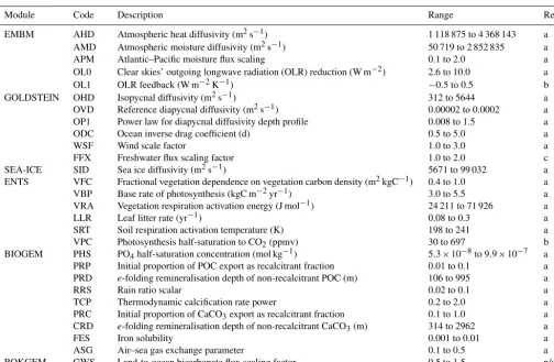
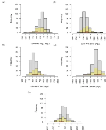
Although our ensemble varies many of the parameters thought to contribute to variability in glacial–interglacial at-mospheric CO2, not all sources of uncertainty can be cap-tured. We estimate, based on our expert opinion, that up to ∼60 ppmv of1CO2could be due to error in our process rep-resentations and processes not included in our model, such as changing marine bacterial metabolic rate, wind speed (via its effect on gas transfer) and Si fertilisation. This is not a com-prehensive assessment, however, as our model also does not include processes such as the effect of changing winds on ocean circulation (Toggweiler et al., 2006), Si leakage (Mat-sumoto et al., 2002, 2013, 2014), the effect of decreasing sea surface temperatures (SSTs) on CaCO3production (Iglesias-Rodriguez et al., 2002) or changing oceanic PO4inventory (Menviel et al., 2012). We focus our analyses on the subset of the ensemble with1CO2between∼ −90 and−30 ppmv (Table 2), treating each value in this range as equally plausi-ble. To test the robustness of diagnosed relationships, we also briefly compare the response of this subset (ENS104) with the response of the ensemble with no1CO2filter (ENS315) and the response of the ensemble with a more negative 1CO2 filter (ENS16). In ENS16, the upper 1CO2 limit is set to ∼ −60 ppmv, roughly equivalent to allowing for an extra at-mospheric CO2 decrease due to changing marine bacterial metabolic rate, wind speed (via its effect on gas transfer) and Si fertilisation, between the best and upper estimate of Ko-hfeld and Ridgwell (2009). The 1CO2distribution in each subset or ensemble is shown in Fig. 1.
Figure 1. LGM change in atmospheric CO2 distribution. The ENS315response is shown in grey, the ENS104ensemble response in yellow and the ENS16 ensemble response in orange. The same colour legend applies to all figures in the paper.
3 Results and discussion
3.1 Pre-industrial simulations
Comparison of the pre-industrial response of ENS315 (i.e. the original, non-1CO2 filtered ensemble) against the pre-industrial ensemble response of Holden et al. (2013a) con-firms that the two are very similar. We additionally evaluate ENS315 against a few additional pre-industrial metrics (see Sect. S2) and find responses that can be deemed plausible, following the design principles for the ensemble, outlined in Holden et al. (2013a).
3.2 LGM simulations
3.2.1 Climate, sea level and ocean circulation Temperature
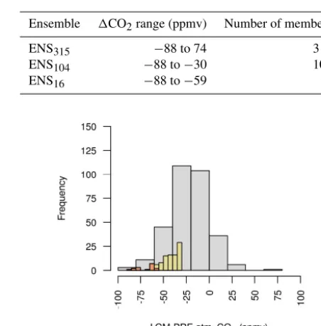
The ENS104 mean LGM surface air temperature (SAT) anomaly (1SAT) is −4.6±1.7, and the range is −2.5 to −10.4◦C. The mean is close to the observed1SAT of−4±
Figure 2.LGM change in surface air temperature and sea surface temperature(a–b)distributions.
data-constrained model estimate (Schmittner et al., 2011) and within the range of estimates inferred from proxy data (MARGO Project Members 2009 in Masson-Delmotte et al., 2013). There is a positive correlation between 1SAT and 1CO2 (r=0.75, 0.05 significance level henceforth), most likely reflecting the radiative impact of atmospheric CO2on SAT, as well as the effect of changing SAT on1CO2. As sug-gested above, decreasing SST may contribute to decreasing CO2via the CO2solubility temperature dependence. Chang-ing SAT may also affect 1CO2 via its effects on sea ice, ocean circulation, terrestrial and marine productivity (see below). The positive correlation is reproduced in ENS315 (r=0.74), and as shown in Fig. 2,1SAT and1SST tend to be less negative in ENS315than in ENS104. In ENS16,1SAT and1SST are from the extreme or at least lower end of the ENS104range.
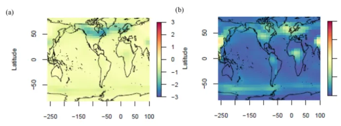
The ENS104mean1SAT and1SST spatial distributions are shown in Fig. 3. In line with observations (Annan and Hargreaves, 2013), the largest SAT decreases (>10◦C) are simulated over the Laurentide and Eurasian ice sheets. The Equator-to-pole temperature gradient is also broadly repro-duced. The largest SST decreases (≥4◦C) are found in the North Atlantic and northeast Pacific, with more limited cool-ing (≤ −2◦C) in the tropics and polar regions, again consis-tent with observations. However, the largest SST decreases ought to also be found in the Southern Hemisphere midlati-tudes, whereas the simulated cooling is more moderate.
Salinity
The ENS104mean percentage increase in LGM salinity (and DIC, ALK, PO4, etc.) due to decreasing sea level is 2.84± 0.62 %S, and the range is 2 %S to 4 %S. There is no signifi-cant relationship between %S and1CO2in either ENS104or ENS315, and the distribution of %S is similar in ENS104and in both ENS315and ENS16(Fig. 4).
Sea ice
The ENS104mean LGM global annual sea ice area anomaly (1SIA) is 18.6±7.4 million km2, and the range is 9.9 to 44 million km2. There is a negative correlation between 1SIA and1SAT (r= −0.97) and between1SIA and1CO2 (r= −0.74). The negative correlation between 1SIA and 1CO2 likely reflects the impact of changing atmospheric CO2 on1SIA but may also include a smaller contribution from changing sea ice area to1CO2. Increasing LGM sea ice area could, for instance, have capped the outgassing of CO2 from the ocean, particularly in the Southern Ocean, and also reduced the net ocean–atmosphere CO2flux by de-creasing the AMOC strength (see below). The negative cor-relation between1SIA and1SAT, and between1SIA and 1CO2, is reproduced in ENS315(r= −0.96 andr= −0.74, respectively).1SIA in ENS104also tends to be higher than in ENS315and smaller than in ENS16(Fig. 5).
As shown in Fig. 6, fractional sea ice cover increases in all regions where sea ice is present in pre-industrial simula-tions, although the largest increases take place in the North Atlantic.
Precipitation
Figure 3.LGM change in surface air temperature(a–b)and sea surface temperature(c–d)(◦C) ENS104mean(a, c)and standard deviation(b,
d).
Figure 4.Percentage increase in LGM salinity due to decreasing sea level distribution.
suggest that the simulated precipitation changes over Europe and equatorial Africa are of the right direction, while precipi-tation changes over western Siberia at least ought to be nega-tive. The sign of the precipitation changes over North Amer-ica is mostly consistent with observations, which record neg-ative changes over most of the continent. However, positive changes, which are also observed, are not captured. Although not shown here, comparison of the ENS104mean against the ENS315mean suggests that the precipitation patterns in the two are very similar, but the decreases generally tend to be higher in the ENS104 mean. The precipitation decreases in ENS104conversely tend to be smaller than in ENS16.
Figure 5.LGM change in global sea ice area distribution.
Ocean circulation
an-Figure 6.LGM-PRE(a–b)and PRE(c–d)fractional sea ice cover ENS104means(a, c)and standard deviations(b, d).
Figure 7.LGM change in precipitation rate (mm d−1) ENS104mean(a)and standard deviation(b).
ticlockwise flow of Antarctic water. A negative1ψmin con-versely represents an LGM increase in cell strength. How-ever, the difference between the LGM and PRE Atlantic AABW here is not statistically significant. The range of 1ψmin is−4.3 to 4.3 Sv, roughly comparable to the range of 1ψminpredicted in Weber et al. (2007) (see also Muglia and Schmittner, 2015) but excluding the much larger ψmin increase predicted by Kim et al. (2003), for example. As shown in Fig. 9, the northern limit of the ENS104mean LGM AABW cell is roughly at the same latitude as in the pre-industrial simulations. The maximum depth reached by the ensemble mean AMOC base is also similar to pre-industrial. Observations (Lynch-Stieglitz et al., 2007; Lippold et al., 2012; Gebbie, 2014; Böhm et al., 2015), conversely, suggest
that the LGM AMOC shoaled to less than 2 km, raising its base depth by 2500 and 600 m at the north and south ends of the return flow, respectively. The LGM AABW, in turn, is thought to have filled the deep Atlantic below 2 km, reaching as far north as 65◦N, which is approximately 25◦north of its modern northern limit (Oppo et al., 2015).
relation-Figure 8.LGM change inψmaxandψmin(a–b)distributions.
Figure 9.LGM(a–b)and PRE(c–d)Atlantic overturning stream function (Sv) ENS104means(a, c)and standard deviations(b, d).
ship between1ψmin and1CO2(r= −0.42). The relation-ships are reproduced in ENS315 (r=0.59 and r= −0.36, respectively). We additionally find, in both ENS104 and ENS315, negative correlations between1ψmax and 1ψmin (r= −0.62 and −0.63), 1ψmin and1SAT (r= −0.4 and −0.4), and 1ψmax and 1SIA (r= −0.62 and −0.66), as well as positive correlations between1ψmaxand1SAT (r= 0.68 and 0.66), and1ψminand1SIA (r=0.37 and 0.42). Based on these relationships, we hypothesise that increasing LGM AABW strength led to an expansion of the AABW cell. The latter in turn restricted the AMOC to lower depths and reduced its overturning rate (e.g. Shin et al., 2003). The increase in AABW strength was likely driven by increases
in sea ice enhancing brine rejection. Sea ice increases in the North Atlantic may have additionally weakened the AMOC cell by locally reducing deep convection.
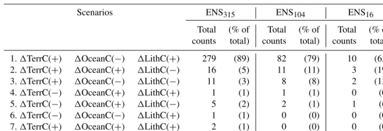
Table 3.LGM-PRE carbon partitioning scenarios in ENS315, ENS104and ENS16.
Scenarios ENS315 ENS104 ENS16
Total (% of Total (% of Total (% of counts total) counts total) counts total)
1.1TerrC(+) 1OceanC(−) 1LithC(+) 279 (89) 82 (79) 10 (63) 2.1TerrC(+) 1OceanC(+) 1LithC(−) 16 (5) 11 (11) 3 (19) 3.1TerrC(+) 1OceanC(−) 1LithC(−) 11 (3) 8 (8) 2 (13) 4.1TerrC(−) 1OceanC(+) 1LithC(+) 1 (1) 1 (1) 0 (0) 5.1TerrC(−) 1OceanC(+) 1LithC(−) 5 (2) 2 (1) 1 (6) 6.1TerrC(−) 1OceanC(−) 1LithC(+) 1 (1) 0 (0) 0 (0) 7.1TerrC(+) 1OceanC(+) 1LithC(+) 2 (1) 0 (0) 0 (0)
have caused the deep ocean to become more stratified, allow-ing more DIC to accumulate at depth and promotallow-ing further CaCO3 dissolution. A decrease in NADW formation could have additionally lowered atmospheric CO2by reducing CO2 outgassing at the ocean surface and reducing the burial rate of deep-sea CaCO3due to the concomitant increase in deep-sea DIC accumulation. Further investigation is, however, re-quired to confirm these causal relationships.
3.2.2 Terrestrial biosphere, ocean and lithospheric carbon
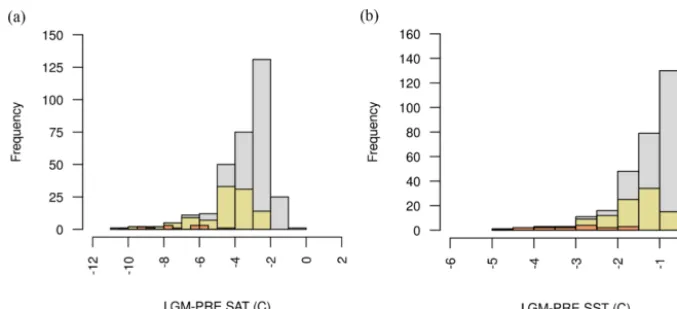
As shown in Fig. 10, most of the ensemble members in ENS104 predict an LGM increase in terrestrial biosphere (1TerrC) and lithospheric1 (1LithC) carbon inventory and a decrease in ocean carbon inventory (1OceanC). The re-maining ensemble members predict one of four other sce-narios of carbon partitioning, with the second most common scenario (11 % of ensemble members) being increasing ter-restrial carbon and decreasing ocean and lithospheric carbon (Table 3). Similar patterns can also be observed in ENS315 and ENS16. A likely explanation for scenario 1 (increase in terrestrial biosphere and lithospheric carbon, decrease in ocean carbon) is that reduced soil decomposition (see below) causes a flux of CO2from the atmosphere to the land, lead-ing to an immediate outgasslead-ing of CO2from the ocean to re-move the atmosphericpCO2difference. The CO2outgassing also leads to an increase in surface [CO23−] and subsequently deep ocean [CO23−], which reduces CaCO3dissolution (and increases lithospheric carbon). The increase in CaCO3burial in turn decreases [CO23−] and increases [CO2], which is com-municated back to the surface, with a resultant increase in atmospheric CO2(Kohfeld and Ridgwell, 2009). The above explanation is of course only part of the explanation for this dominant carbon partitioning scenario, with physical mecha-nisms also expected to play a role, in addition to any changes
1The1LithC stems from changes in the deep-sea CaCO 3burial flux and/or CaCO3 weathering/shallow water deposition flux and was initially calculated to ensure that carbon was being conserved over the LGM simulation.
in ocean productivity and changes in land carbonate weath-ering (see below).
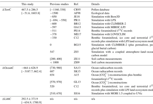
The ENS104 mean 1TerrC, 1OceanC and 1LithC, the signs of which are consistent with scenario 1, are reported in Table 4, alongside previous estimates from observational data- and model-based studies. From here, we can see that the mean1TerrC is only aligned with a handful of estimates and no studies so far report a negative 1OceanC. Instead, 1OceanC is estimated to be positive, primarily based on bon isotope data. The loss of hundreds of petagrams of car-bon from the ocean in response to terrestrial carcar-bon growth has, however, been previously proposed (e.g. Zimov et al., 2006). Moreover, if we assume that 90 % of the atmospheric CO2 perturbation caused by the increase in terrestrial bio-sphere carbon reported in Table 4 gets removed by the ocean and sediments, the change in ocean carbon would be nega-tive, even after adding the remaining carbon to be lost from the atmosphere to the ocean. We discuss what these results would likely mean for carbon isotope data in Sect. 3.2.6.
pre-Figure 10.LGM change in vegetation(a), soil (b), terrestrial (vegetation plus soil)(c), ocean(d)and lithospheric(e)carbon inventory distributions.
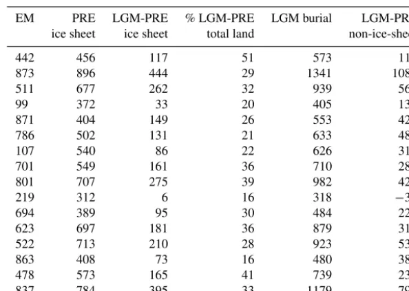
vious studies, irrespective of what the response of the ter-restrial biosphere is to the LGM climate and CO2forcings. O’ishi and Abe-Ouchi (2011), for instance, estimated that the LGM climate is responsible for the loss of 502 PgC of terrestrial carbon, while another 388 PgC is removed by the ice sheets. Zeng (2003) conversely proposed that 431 PgC is preserved under the ice sheets at the LGM. This number in-cludes 315 PgC present during the interglacial and another 116 PgC accumulated in response to the glacial climate forc-ings, prior to insulation of the terrestrial carbon from the at-mosphere by the ice sheet coverage. Here, analysis of ENS16 suggests that during the 1000 years of LGM ice sheet build-up, the terrestrial carbon inventory in the areas to be occu-pied by the ice sheets increases by between 6 and 444 PgC,
yielding LGM “ice sheet or burial” carbon inventories be-tween 318 and 1341 PgC (Table 5). This increase accounts for less than half of the total LGM change in terrestrial car-bon (i.e.1TerrC) in the majority of simulations. However, if this burial carbon were to have been destroyed rather than preserved,1TerrC would be negative in all but three simu-lations, as opposed to positive in all but one simulation (Ta-ble 5).
Table 4. LGM-PI difference in terrestrial (1TerrC), ocean (1OceanC) and lithospheric (1LithC) carbon inventory (PgC) in this study (ENS104 mean, standard deviation and range) and previous studies. CR95 is Crowley (1995), AF98 is Adams and Faure (1998), Z03 is Zeng (2003), ZI09 is Zimov et al. (2009), PR11 is Prentice et al. (2011), ZE11 is Zech et al. (2011), BR12 is Brovkin et al. (2012), CI12 is Ciais et al. (2012), GL13 is Goodwin and Lauderdale (2013), OA13 is O’ishi and Abe-Ouchi (2013), SA is Sarnthein et al. (2013), PE14 is Peterson et al. (2014), AL15 is Allen et al. (2015), BG15 is Brovkin and Ganopolski (2015), SK15 is Skinner et al. (2015), SS16 is Schmittner and Somes (2016), ME17 is Menviel et al. (2017) and JE18 is Jeltsch-Thömmes et al. (2019).
This study Previous studies Ref. Details
1TerrC 467.5±286.5 [−51.6,1603.8]
[−1160,530] −1500 −850
[−694,−550] −600 −597 −511 −378
−330
0
CR95 AF98 JE18 PR11 BR12 OA13 PE14 ME17 C12
BG15
Pollen database Ecological data Simulation with Bern3D Simulation with LPX Simulation with CLIMBER-2 Simulation with MIROC-LPJ Benthic foraminiferalδ13C records Simulation with LOVECLIM
Benthic foraminiferal, ice core and terrestrial δ13C records plus simulation with LPJ land ecosystem model Simulation with CLIMBER-2 (plus permafrost, peat, glacial burial carbon)
547 Z03 Simulation with a coupled atmosphere–land–ocean– carbon model
[200,400] ZE11 Soil carbon measurements <1000 ZI09 Soil carbon measurements
1OceanC −664±626.9 [−3187.7,662.4]
[730,980] 687 654
[570,970]
SA13 SK15 A15
GL13
Ocean radiocarbon records Ocean radiocarbon records
Ocean [CO23−] reconstructions plus benthic foraminiferalδ13C records
Ocean [CO23−] reconstructions
520 C12 Benthic foraminiferal, ice core and terrestrial δ13C records plus simulation with LPJ land ecosystem model [510,670] SS16 Simulation with MOBI 1.5 coupled to UVic
1LithC 292.5±373.9 [−654.9,1700.9]
n/a n/a n/a
an additional 250–550 PgC (Franzen, 1994) from increased glacial peat accumulation (Zeng, 2003). No observational data-based estimates of the LGM burial carbon inventory are available since only limited evidence exists for organic mate-rial being preserved by ice during glaciations (Franzen, 1994, and references in Weitemeyer and Buffett, 2006). Outside of the ice sheets, increases in the terrestrial carbon inventory in ENS16are mostly due to soil carbon, which increases in all simulations. Vegetation carbon, conversely, decreases in the majority of simulations. Our range of carbon changes outside of the ice sheet areas include the 198 PgC increase predicted by Zeng (2003) as a result of reduced soil respiration.
Although not evaluated directly, it is likely that similar ice sheet/non-ice-sheet terrestrial carbon proportions than in ENS16are found in ENS104and ENS315because of the simi-lar climate change distributions in all three instances (see ear-lier sections). Although not shown here, the spatial distribu-tion of1TerrC in ENS16is also similar to that of the ENS104
(and ENS315) mean. The spatial distribution of 1TerrC in ENS104is shown in Fig. 11.
107 540 86 22 626 310
701 549 161 36 710 283
801 707 275 39 982 423
219 312 6 16 318 −34
694 389 95 30 484 227
623 697 181 36 879 319
522 713 210 28 923 531
863 408 73 16 480 380
478 573 165 41 739 233
837 784 395 33 1179 796
Laurentide and Eurasian ice sheet areas are of the wrong sign, except in northwest North America, since these stud-ies assume the complete destruction of vegetation and soils in ice sheet areas. Discrepancies between the ENS104and ob-servations further arise from the rainforest regions, where the ensemble mean predicts terrestrial biosphere carbon density changes between−5 and 10 kgC m−2, well above observed changes of∼ −23 kgC m−2. It is important to note, however, that as suggested in Zeng (2007), the rate of decomposition of soil carbon at the LGM may have been slower than as-sumed in pollen data-based studies. The largest increases in terrestrial carbon density (∼40 kgC m−2) produced by the ensemble mean are comparable to those found in areas with permafrost growth (Zimov et al., 2006). However, the peaks are potentially misplaced, being located within and south of the Laurentide and Eurasian ice sheet covered areas, rather than in eastern Siberia and Alaska. Alternatively, terrestrial carbon increases in eastern Siberia and Alaska are simply underestimated in the ensemble mean and large increases in terrestrial carbon indeed took place within the ice sheet areas during glacial periods.
The large LGM decreases in terrestrial carbon in north-west North America and adjacent Beringia are likely caused by precipitation decreasing comparatively more than SAT and causing the decrease in photosynthesis to exceed the de-crease in soil respiration. However, it is also noteworthy that, although not shown here, the regions with the largest de-creases in terrestrial carbon density, namely northwest North America, Beringia and the Tibetan Plateau area, are also the regions with the largest terrestrial carbon densities in the
pre-industrial ENS315 mean. We further note that the Ti-betan soil carbon peak is overestimated in the latter, and the North American soil carbon peak misplaced, compared to observations. We attribute the first discrepancy to the lack of soil weathering in the model and the inclusion of land use effects in the observational data-based estimate (Holden et al., 2013b; Williamson et al., 2006). The second discrep-ancy is attributed to the lack of explicit representation of per-mafrost and the absence of moisture control on soil respira-tion (Williamson et al., 2006).
3.2.3 Ocean primary productivity
Figure 11.LGM vegetation(a–b), soil(c–d)and total terrestrial carbon changes(e–f)ENS104mean(a, c)and standard deviation(b, d). Units are kgC m−2.
AMOC cell would also inhibit the transfer of nutrients from the deep ocean to the surface. A negative correlation can ad-ditionally be found between1POCexpand1SIA (r= −0.55 and−0.6), probably because no primary production occurs beneath the sea ice surface. Increasing sea ice area at the LGM therefore leads to decreasing POC export flux. This would also explain the largest ENS104 mean decreases in POC export flux, shown in Fig. 13, coinciding with increases in sea ice fraction.
The largest ENS104 LGM increases in POC export flux conversely occur at around 50◦S, roughly in front of the Antarctic sea ice margins. Increases in POC export are also simulated close to the North Pacific and Atlantic sea ice margins, as well as in the eastern equatorial Pacific and the southwest Atlantic upwelling region. The increases in POC export flux at the sea ice margins are likely caused by the advection of unutilised nutrients from underneath the sea ice. However, they may additionally be due to the enhanced iron availability from the increased supply of aeolian dust,
particularly in the Southern Ocean and North Pacific since these are strongly limited by iron (Ridgwell et al., 2007). Iron fertilisation may also explain the increases in POC ex-port flux in the eastern equatorial Pacific and in the south-west Atlantic upwelling region. Comparison against obser-vations suggests that the ensemble mean POC flux changes immediately north, and south of the Antarctic sea ice mar-gins align with observations of increased and reduced marine productivity in the subantarctic (∼45 to 60◦N) and South-ern Ocean, respectively (Kohfeld, 2005; Kohfeld et al., 2013; Jaccard et al., 2013; Martínez-García et al., 2014). The sim-ulated decreases in export flux in the Arctic and subarctic Atlantic (i.e. above approximately 50◦N), and the increases in export flux immediately south of 50◦N are also in
agree-ment with previous reconstructions (Kohfeld, 2005; Radi and de Vernal, 2008). The mostly lower LGM export fluxes at the Equator and in the South Atlantic are conversely incon-sistent with the observational data of Kohfeld (2005). The decreases may be caused by the increases in productivity in high-nutrient, low-chlorophyll (HNLC) regions reducing the phosphate (the other limiting nutrient in GENIE-1 be-sides iron) availability for photosynthesis in other regions. They may additionally be due to the model not simulating en-hanced nutrient inventories in response to enen-hanced weather-ing or reduced shallower water deposition of organic matter. The model also does not vary wind speed, which may have resulted in stronger tropical upwelling in the Atlantic at the LGM. The evidence is more ambiguous (or missing) for the Pacific (Jaccard et al., 2010; Kohfeld and Chase, 2011; Ko-hfeld, 2005; Costa et al., 2016) and Indian oceans (KoKo-hfeld, 2005; Singh et al., 2011) and is therefore not discussed in more detail here.
3.2.4 Carbonate weathering and shallow water deposition
The ENS104 mean land-to-ocean bicarbonate flux scaling factor (GWS) is 1.16±0.24 (corresponding to a percent-age change in the land-to-ocean bicarbonate flux, %LOC, of 38.67), and the range is 0.52 to 1.5 (corresponding to
Figure 14.Land-to-ocean bicarbonate flux scaling factor (GWS) distributions.
a %LOC between −49.33 and 50). As shown in Fig. 14, the GWS in ENS104 tends to be larger than in ENS315 and smaller than in ENS16. There is also a negative correlation between GWS and1CO2(r= −0.52) in ENS315, suggest-ing that increassuggest-ing the input of bicarbonate to the ocean leads to a decrease in CO2by raising the inventories of ALK and DIC in a 2:1 ratio. In ENS104, however,ris below the 0.05 significance level, suggesting that it is less important.
3.2.5 Deep-sea carbonate burial
The ENS104 mean global deep-sea CaCO3 burial flux anomaly (1CaCO3bur) is 0.036±0.045 PgC yr−1 and the range is−0.098 to 0.139 PgC yr−1. The mean value is ap-proximately 3 times larger than the observed value (Catubig et al., 1998), although the latter still falls within the range of simulated values. As shown in Fig. 15, 1CaCO3bur in
Figure 15.LGM change in deep-sea sediment CaCO3burial flux distributions.
deep ocean CO23−will eventually increase. The latter in turn would cause the saturation horizon to fall, allowing CaCO3 to accumulate over greater areas (which are now exposed to undersaturated waters) (Sigman and Boyle, 2000). The in-put of ALK to the surface ocean would also increase the rate of CaCO3export production (enhancing the sediment depo-sition flux of CaCO3), since as discussed in Chikamoto et al. (2008), the latter is proportional to the production rate of POC (which is equal to the POC export flux), together with the sea surface saturation state with respect to CaCO3, in GENIE-1. There is indeed also a positive correlation be-tween %LOC and the global change in CaCO3export flux (r=0.27 and 0.4), and between the latter and 1CaCO3bur
(r=0.34 and 0.45) in both ENS104and ENS315.
The ENS104 mean spatial distribution of 1CaCO3bur is
shown in Fig. 16. Relatively large increases in burial flux (≥0.5×10⁻⁵mol cm−2yr−1) can be found at around 50◦S, in the North Pacific and to a lesser extent the North Atlantic. In other regions, the burial flux is significantly lower or neg-ative, with the largest losses (≤ −0.5×10⁻⁵mol cm−2yr−1) occurring in the North Atlantic and arctic regions. The only exception is the western North Atlantic, which exhibits a large increase in burial. A comparison of the results against the reconstructions of Catubig et al. (1998) is somewhat dif-ficult, as the coverage is poor but overall CaCO3burial was higher in the North Atlantic and the Pacific, and lower in the tropical and South Atlantic, and the Indian Ocean and South-ern Ocean.
3.2.6 Other paleoproxies
As shown in Table 4, a frequent argument for a lower glacial terrestrial carbon inventory is the reconstructed mean glacial oceanδ13C value of approximately 0.35 ‰ lower than present due to the fact that plants discriminate against 13C during photosynthesis. In our simulations, conversely, it fol-lows that the increase in glacial terrestrial carbon inventory would have resulted in an increase in oceanδ13C. Decreasing
SSTs and increasing CaCO3 weathering would have, more-over, likely raised it further (in the first instance, by enhanc-ing fractionation at the air–sea interface, and in the second instance, through the input of isotopically heavy weathering products). However, as noted in Zeng (2007), the interpreta-tion of theδ13C value can be complicated by factors such as the impact of enhanced glacial carbonate ion concentrations onδ13C in foramifera shells (Lea et al., 1999). In addition, there are other processes in our model which may have coun-teracted at least part of the increase in oceanδ13C. These in-clude reduced marine productivity (e.g. Zimov et al., 2009), as phytoplankton discriminate against13C during photosyn-thesis, giving the marine organic carbon reservoir a lowδ13C. However, we note that the sign of this impact would addition-ally depend on the associated changes in organic matter rem-ineralisation and burial. Another relevant process is greater sea ice area, which can lower the ocean δ13C by reducing the air–sea gas exchange and therefore the net transfer of13C into the ocean (Stephen and Keeling, 2000). Moreover, we propose that adding missing processes could have decreased oceanδ13C even further. These include weaker surface winds (while in our model these are fixed), again through reduced air–sea gas exchange (Menviel et al., 2015), as well as en-hanced weathering and reduced deposition of organic car-bon at continental margins due to lower sea levels (Wall-mann, 2014). Yet, further research is required here as one recent study suggests that taking into account these processes would most likely not (the possibility is not completely ruled out) allow reconciliation of a positive1TerrC with the ob-served mean glacial oceanδ13C value (Jeltsch-Thömmes et al., 2019).
into our model (Kohfeld and Ridgwell, 2009; Menviel et al., 2012).
4 Conclusions
We have used an uncertainty-based approach to investigat-ing the LGM atmospheric CO2 drop by simulating it with a large ensemble of parameter sets and exploring the range of possible responses. Despite our ensemble varying many of the parameters thought to contribute to variability in glacial–interglacial atmospheric CO2, we estimated that up to∼60 ppmv of1CO2could be attributed to processes not included in our model and error in our process representa-tions. As a result, we treated 1CO2 between ∼ −90 and −30 ppmv as equally plausible and focused on describing the responses of the subset of simulations with this1CO2. We found the range of responses to be large, including the presence of five different ways of achieving a plausible 1CO2 in terms of the sign of individual carbon reservoir changes. However, several dominant changes could be de-tected. Namely, the LGM atmospheric CO2decrease tended to predominantly be associated with decreasing SSTs, in-creasing sea ice area, a weakening of the AMOC, a strength-ening of the AABW cell in the Atlantic Ocean, a decreasing ocean biological productivity, an increasing CaCO3 weather-ing flux and an increasweather-ing deep-sea CaCO3burial flux. The majority of our simulations also predicted an increase in ter-restrial carbon, coupled with a decrease in ocean and an in-crease in lithospheric carbon.The increase in terrestrial car-bon, which is uncommon in LGM simulations, was attributed to reduced soil respiration in response to the climate forcings, as well as our choice to preserve rather than destroy carbon that accumulates in ice sheet areas. The dominant changes were broadly in agreement with observations and paleoprox-ies other than carbon isotope and oxygen data, which we did not evaluate directly. However, we advise more detailed com-parisons in future studies. It is also likely that our results can only be reconciled with carbon isotope and oxygen data if processes currently missing from our model are taken into account.
Code and data availability. GENIE-1 was checked out via https: //source.ggy.bris.ac.uk/wiki/GENIE (last access: May 2019) using Subversion (SVN). The simulations described here are with release version 2-8-0. In addition to the source code, several packages and applications such as the NetCDF libraries are required by GENIE-1 (University of Bristol Geography Source, 2014).
The way in which GENIE-1 is run manually is as described in Ridgwell (2012) for the GENIE developmental variant cGE-NIE: the basic flavour and configuration of GENIE-1 is run from ∼/genie/genie-mainby issuing the command
./genie.job
genie.jobis a shell script which determines the basic (“base”) configuration of the model. A different flavour and configuration of the model is obtained by specifying a different base configuration file:
./genie.job -f example.xml
where example.xml is a specified model configuration
(/flavour) .xmlfile (Ridgwell, 2012).
Appendix A: The OLR feedback parameter
The ensemble parameter OL1 is varied through all stages but stage 1. OL1 describes the unmodelled response of clouds to global average temperature change and corresponds to the KLW1constant in the equation below (Eq. 1 in Holden et al., 2010a):
L∗out=Lout(T , q)−KLW0−KLW11T , (A1)
whereLout(T , q) is the unmodified “clear skies” OLR term of Thompson and Warren (1982),KLW0is the clear-sky out-going long-wave radiation parameter (OL0), representing the effects of clouds on the unmodified OLR (withKLW0 only ever taking positive values), and1T corresponds to the dif-ference between the globally averaged surface air tempera-ture and the equilibrium pre-industrial temperatempera-ture (Holden et al., 2010a).
Acknowledgements. This work made use of the Darwin Su-percomputer of the University of Cambridge High Performance Computing Service (HPCS). Krista M. S. Kemppinen thanks staff at HPCS for their technical support, and Antara Banerjee and Alex Archibald for help with R. The manuscript was greatly im-proved by comments from an anonymous reviewer.
Financial support. This research has been supported by the UK Natural Environment Research Council (NERC) through funding for the project DESIRE (grant no. NE/E007554/1).
Review statement. This paper was edited by Laurie Menviel and reviewed by Pearse Buchanan and two anonymous referees.
References
Adams, J. M. and Faure, H.: A new estimate of changing carbon storage on land since the last glacial maximum, based on global land ecosystem reconstruction, Global Planet. Change, 16–17, 3–24, https://doi.org/10.1016/S0921-8181(98)00003-4, 1998. Adkins, J. F., Mcintyre, K., and Schrag, D. P.: The Salinity,
Temper-ature, andδ18O of the Glacial Deep Ocean, Science, 298, 1769– 1773, https://doi.org/10.1126/science.1076252, 2002.
Alder, J. R. and Hostetler, S. W.: Global climate simulations at 3000-year intervals for the last 21 000 years with the GEN-MOM coupled atmosphere–ocean model, Clim. Past, 11, 449– 471, https://doi.org/10.5194/cp-11-449-2015, 2015.
Allen, K. A., Sikes, E. L., Hönisch, B., Elmore, A. C., Guilder-son, T. P., Rosenthal, Y., and AnderGuilder-son, R. F.: Southwest Pa-cific deep water carbonate chemistry linked to high south-ern latitude climate and atmospheric CO2 during the Last Glacial Termination, Quaternary Sci. Rev., 122, 180–191, https://doi.org/10.1016/j.quascirev.2015.05.007, 2015.
Anderson, R. F., Ali, S., Bradtmiller, L. I., Nielsen, S. H. H., Fleisher, M. Q., Anderson, B. E., and Burckle, L. H.: Wind-Driven Upwelling in the Southern Ocean and the Deglacial Rise in Atmospheric CO2, Science, 323, 1443–1448, https://doi.org/10.1126/science.1167441, 2009.
Annan, J. D. and Hargreaves, J. C.: Efficient identification of ocean thermodynamics in a physical/biogeochemical ocean model with an iterative Importance Sampling method, Ocean Model., 32, 205–215, https://doi.org/10.1016/j.ocemod.2010.02.003, 2010.
Berger, A.: Long-term variations of daily insolation and quaternary climatic changes, J. Atmos. Sci., 35, 2362–2367, 1978. Böhm, E., Lippold, J., Gutjahr, M., Frank, M., Blaser, P., Antz,
B., Fohlmeister, J., Frank, N., Andersen, M. B., and Deininger, M.: Strong and deep Atlantic meridional overturning cir-culation during the last glacial cycle, Nature, 517, 73–76, https://doi.org/10.1038/nature14059, 2015.
Bopp, L., Kohfeld, K. E., Le Quéré, C., and Au-mont, O.: Dust impact on marine biota and atmo-spheric CO2 during glacial periods, Paleoceanogra-phy, 18, 1046, https://doi.org/10.1029/2002PA000810, https://doi.org/10.1029/2002PA000810, 2003.
Bouttes, N., Paillard, D., and Roche, D. M.: Impact of brine-induced stratification on the glacial carbon cycle, Clim. Past, 6, 575–589, https://doi.org/10.5194/cp-6-575-2010, 2010.
Bouttes, N., Paillard, D., Roche, D. M., Brovkin, V., and Bopp, L.: Last Glacial Maximum CO2 and δ13C suc-cessfully reconciled, Geophys. Res. Lett., 38, L02705, https://doi.org/10.1029/2010gl044499, 2011.
Brady, E. C., Otto-Bliesner, B. L., Kay, J. E., and Rosenbloom, N.: Sensitivity to glacial forcing in the CCSM4, J. Climate, 26, 1901–1925, https://doi.org/10.1175/JCLI-D-11-00416.1, 2013. Braconnot, P., Otto-Bliesner, B., Harrison, S., Joussaume, S.,
Pe-terchmitt, J.-Y., Abe-Ouchi, A., Crucifix, M., Driesschaert, E., Fichefet, Th., Hewitt, C. D., Kageyama, M., Kitoh, A., Laîné, A., Loutre, M.-F., Marti, O., Merkel, U., Ramstein, G., Valdes, P., Weber, S. L., Yu, Y., and Zhao, Y.: Results of PMIP2 coupled simulations of the Mid-Holocene and Last Glacial Maximum – Part 1: experiments and large-scale features, Clim. Past, 3, 261– 277, https://doi.org/10.5194/cp-3-261-2007, 2007.
Brovkin, V. and Ganopolski, A.: The role of the terrestrial biosphere in CLIMBER-2 simulations of the last glacial CO2cycles, Nova Act. LC NF, 121, 43–47, 2015.
Brovkin, V., Hofmann, M., Bendtsen, J., and Ganopolski, A.: Ocean biology could control atmospheric δ13C during glacial-interglacialcycle, Geochem. Geophy. Geosy., 3, 1027, https://doi.org/10.1029/2001GC000270, 2002.
Brovkin, V., Ganopolski, A., Archer, D. and Rahmstorf, S.: Low-ering of glacial atmospheric CO2 in response to changes on oceanic circulation and marine biogeochemistry, Paleoceanogra-phy, 22, A4202, https://doi.org/10.1029/2006PA001380, 2007. Brovkin, V., Ganopolski, A., Archer, D., and Munhoven, G.: Glacial
Buchanan, P. J., Matear, R. J., Lenton, A., Phipps, S. J., Chase, Z., and Etheridge, D. M.: The simulated climate of the Last Glacial Maximum and insights into the global marine carbon cycle, Clim. Past, 12, 2271–2295, https://doi.org/10.5194/cp-12-2271-2016, 2016.
Catubig, N. R., Archer, D. E., Francois, R., DeMenocal, P., Howard, W., and Yu, E. F.: Global deep-sea burial rate of calcium car-bonate during the Last Glacial Maximum, Paleoceanography, 13, 298–310, https://doi.org/10.1029/98PA00609, 1998.
Chikamoto, M. O., Matsumoto, K., and Ridgwell, A.: Response of deep-sea CaCO3sedimentation to Atlantic meridional over-turning circulation shutdown, J. Geophys. Res.-Biogeo., 113, G03017, https://doi.org/10.1029/2007JG000669, 2008. Chikamoto, M. O., Abe-Ouchi, A., Oka, A., Ohgaito, R., and
Tim-mermann, A.: Quantifying the ocean’s role in glacial CO2 reduc-tions, Clim. Past, 8, 545–563, https://doi.org/10.5194/cp-8-545-2012, 2012.
Ciais, P., Tagliabue, A., Cuntz, M., Bopp, L., Scholze, M., Hoff-mann, G., Lourantou, A., Harrison, S. P., Prentice, I. C., Kel-ley, D. I., Koven, C., and Piao, S. L.: Large inert carbon pool in the terrestrial biosphere during the Last Glacial Maximum, Nat. Geosci., 5, 74–79, https://doi.org/10.1038/ngeo1324, 2012. Ciais, P., Sabine, C., Bala, G., Bopp, L., Brovkin, V., Canadell, J.,
Chhabra, A., DeFries, R., Galloway, J., Heimann, M., Jones, C., Quéré, C. Le, Myneni, R. B., Piao, S., and Thornton, P.: Carbon and Other Biogeochemical Cycles, in: Climate Change 2013: The Physical Science Basis. Contribution of Working Group I to the Fifth Assessment Report of the Intergovernmental Panel on Climate Change, edited by: Stocker, T. F., Qin, D., Plattner, G.-K., Tignor, M., Allen, S. G.-K., Boschung, J., Nauels, A., Xia, Y., Bex, V., and Midgley, P. M., Cambridge University Press, Cam-bridge, United Kingdom and New York, NY, USA, 2013. Colbourn, G.: Weathering effects on the carbon cycle in an Earth
System Model, PhD thesis, School of Environmental Sciences, University of East Anglia, UK, 2011.
Costa, K. M., McManus, J. F., Anderson, R. F., Ren, H., Sig-man, D. M., Winckler, G., Fleisher, M. Q., Marcantonio, F., and Ravelo, A. C.: No iron fertilization in the equatorial Pa-cific Ocean during the last ice age, Nature, 529, 519–522, https://doi.org/10.1038/nature16453, 2016.
Crocket, K. C., Vance, D., Foster, G. L., Richards, D. A., and Tranter, M.: Continental weathering fluxes dur-ing the last glacial/interglacial cycle: insights from the marine sedimentary Pb isotope record at Orphan Knoll, NW Atlantic, Quaternary Sci. Rev., 38, 89–99, https://doi.org/10.1016/j.quascirev.2012.02.004, 2012.
Crowley, T. J.: Ice Age terrestrial carbon changes revisited, Global Biogeochem. Cy., 9, 377–389, https://doi.org/10.1029/95GB01107, 1995.
De La Fuente, M., Skinner, L., Calvo, E., Pelejero, C., and Cacho, I.: Increased reservoir ages and poorly ventilated deep waters in-ferred in the glacial Eastern Equatorial Pacific, Nat. Commun., 6, 7420, https://doi.org/10.1038/ncomms8420, 2015.
Doney, S. C., Lindsay, K., Fung, I., and John, J.: Natural variability in a stable, 1000-yr global coupled climate-carbon cycle simulation, J. Climate, 19, 3033–3054, https://doi.org/10.1175/JCLI3783.1, 2006.
Edwards, N. R. and Marsh, R.: Uncertainties due to transport-parameter sensitivity in an efficient 3-D ocean-climate model,
Clim. Dynam., 24, 415–433, https://doi.org/10.1007/s00382-004-0508-8, 2005.
Ferrari, R., Jansen, M. F., Adkins, J. F., Burke, A., Stewart, A. L., and Thompson, A. F.: Antarctic sea ice control on ocean circula-tion in present and glacial climates, P. Natl. Acad. Sci. USA, 111, 8753–8758, https://doi.org/10.1073/pnas.1323922111, 2014. Foster, G. L. and Vance, D.: Negligible glacial-interglacial variation
in continental chemical weathering rates, Nature, 444, 918–921, https://doi.org/10.1038/nature05365, 2006.
Franzen, L. G.: Are wetlands the key to the ice-age cycle enigma, Ambio, 23, 300–308, 1994.
Franzén, L. G. and Cropp, R. A.: The Peatland/ice age Hypothesis revised, adding a possible glacial pulse trigger, Geogr. Ann. A, 89, 301–330, 2007.
Freeman, E., Skinner, L. C., Tisserand, A., Dokken, T., Timmer-mann, A., Menviel, L., and Friedrich, T.: An Atlantic-Pacific ventilation seesaw across the last deglaciation, Earth Planet. Sc. Lett., 424, 237–244, https://doi.org/10.1016/j.epsl.2015.05.032, 2015.
Gebbie, G.: How much did Glacial North Atlantic Water shoal?, Paleoceanography, 29, 190–209, https://doi.org/10.1002/2013PA002557, 2014.
Goodwin, P. and Lauderdale, J. M.: Carbonate ion concentra-tions, ocean carbon storage, and atmospheric CO2, Global Bio-geochem. Cy., 27, 882–893, https://doi.org/10.1002/gbc.20078, 2013.
Harrison, K. G.: Role of increased marine silica input on paleo-pCO2 levels, Paleoceanography, 15, 292–298, https://doi.org/10.1029/1999PA000427, 2000.
Holden, P. B., Edwards, N. R., Oliver, K. I. C., Lenton, T. M., and Wilkinson, R. D.: A probabilistic calibration of climate sensitiv-ity and terrestrial carbon change in GENIE-1, Clim. Dynam., 35, 785–806, https://doi.org/10.1007/s00382-009-0630-8, 2010a. Holden, P. B., Edwards, N. R., Wolff, E. W., Lang, N. J., Singarayer,
J. S., Valdes, P. J., and Stocker, T. F.: Interhemispheric coupling, the West Antarctic Ice Sheet and warm Antarctic interglacials, Clim. Past, 6, 431–443, https://doi.org/10.5194/cp-6-431-2010, 2010b.
Holden, P. B., Edwards, N. R., Müller, S. A., Oliver, K. I. C., Death, R. M., and Ridgwell, A.: Controls on the spatial dis-tribution of oceanicδ13CDIC, Biogeosciences, 10, 1815–1833, https://doi.org/10.5194/bg-10-1815-2013, 2013a.
Holden, P. B., Edwards, N. R., Gerten, D., and Schaphoff, S.: A model-based constraint on CO2fertilisation, Biogeosciences, 10, 339–355, https://doi.org/10.5194/bg-10-339-2013, 2013b. Iglesias-Rodríguez, M. D., Brown, C. W., Doney, S. C., Kleypas, J.,
Kolber, D., Kolber, Z., Hayes, P. K., and Falkowski, P. G.: Rep-resenting key phytoplankton functional groups in ocean carbon cycle models: Coccolithophorids, Global Biogeochem. Cy., 16, 47-1–47-20, https://doi.org/10.1029/2001GB001454, 2002. Jaccard, S. L., Galbraith, E. D., Sigman, D. M., and Haug, G. H.:
A pervasive link between Antarctic ice core and subarctic Pacific sediment records over the past 800 kyrs, Quaternary Sci. Rev., 29, 206–212, https://doi.org/10.1016/j.quascirev.2009.10.007, 2010.
Productiv-sion, the marine Ge/Si ratio, Global Planet. Change, 33, 139– 153, https://doi.org/10.1016/S0921-8181(02)00067-X, 2002. Joos, F., Gerber, S., Prentice, I. C., Otto-Bliesner, B. L.,
and Valdes, P. J.: Transient simulations of Holocene atmo-spheric carbon dioxide and terrestrial carbon since the Last Glacial Maximum, Global Biogeochem. Cy., 18, GB2002, https://doi.org/10.1029/2003GB002156, 2004.
Kim, S.-J., Flato, G., and Boer, G.: A coupled climate model simulation of the Last Glacial Maximum, Part 2: approach to equilibrium, Clim. Dynam., 20, 635–661, https://doi.org/10.1007/s00382-002-0292-2, 2003.
Kleypas, J. A.: Modeled estimates of global reef habitat and car-bonate production since the last glacial maximum, Paleoceanog-raphy, 12, 533–545, https://doi.org/10.1029/97PA01134, 1997. Kohfeld, K. E.: Role of Marine Biology in
Glacial-Interglacial CO2 Cycles, Science, 308, 74–78, https://doi.org/10.1126/science.1105375, 2005.
Kohfeld, K. E. and Chase, Z.: Controls on deglacial changes in bio-genic fluxes in the North Pacific Ocean, Quaternary Sci. Rev., 30, 3350–3363, https://doi.org/10.1016/j.quascirev.2011.08.007, 2011.
Kohfeld, K. E. and Ridgwell, A.: Glacial-Interglacial Variability in Atmospheric CO2, Surf. Ocean. Atmos. Process., 187, 251–286, https://doi.org/10.1029/2008GM000845, 2009.
Kohfeld, K. E., Graham, R. M., de Boer, A. M., Sime, L. C., Wolff, E. W., Le Quéré, C., and Bopp, L.: Southern Hemi-sphere westerly wind changes during the Last Glacial Maxi-mum: Paleo-data synthesis, Quaternary Sci. Rev., 68, 76–95, https://doi.org/10.1016/j.quascirev.2013.01.017, 2013.
Lambert, F., Tagliabue, A., Shaffer, G., Lamy, F., Winckler, G., Farias, L., Gallardo, L., and De Pol-Holz, R.: Dust fluxes and iron fertilization in Holocene and Last Glacial Maximum climates, Geophys. Res. Lett., 42, 6014–6023, https://doi.org/10.1002/2015GL064250, 2015.
Lea, D. W., Bijma, J., Spero, H. J., and Archer, D.: Implications of a carbonate ion effect on shell carbon and oxygen isotopes for glacial ocean conditions, in: Use of Proxies in Paleoceanography: Examples from the South Atlantic, edited by: Fischer, G. and Wefer, G., Springer-Verlag, Berlin Heidelberg, 513–522, 1999. Lenton, T. M., Marsh, R., Price, A. R., Lunt, D. J., Aksenov, Y.,
Annan, J. D., Cooper-Chadwick, T., Cox, S. J., Edwards, N. R., Goswami, S., Hargreaves, J. C., Harris, P. P., Jiao, Z., Livina, V. N., Payne, A. J., Rutt, I. C., Shepherd, J. G., Valdes, P. J., Williams, G., Williamson, M. S., and Yool, A.: Effects of at-mospheric dynamics and ocean resolution on bi-stability of the
Kissel, C., Marchal, O., Marchitto, T. M., McCave, I. N., Mc-Manus, J. F., Mulitza, S., Ninnemann, U., Peeters, F., Yu, E.-F., and Zahn, R.: Atlantic meridional overturning circula-tion during the Last Glacial Maximum, Science, 316, 66–69, https://doi.org/10.1126/science.1137127, 2007.
Ma, W. and Tian, J.: Modeling the contribution of dissolved organic carbon to carbon sequestration during the last glacial maximum, Geo-Mar. Lett., 34, 471–482, https://doi.org/10.1007/s00367-014-0378-y, 2014.
Mahowald, N. M., Muhs, D. R., Levis, S., Rasch, P. J., Yoshioka, M., Zender, C. S., and Luo, C.: Change in atmospheric mineral aerosols in response to climate: Last glacial period, preindustrial, modern, and doubled carbon dioxide climates, J. Geophys. Res.-Atmos., 111, D10202, https://doi.org/10.1029/2005JD006653, 2006.
Marsh, R., Müller, S. A., Yool, A., and Edwards, N. R.: Incor-poration of the C-GOLDSTEIN efficient climate model into the GENIE framework: “eb_go_gs” configurations of GENIE, Geosci. Model Dev., 4, 957–992, https://doi.org/10.5194/gmd-4-957-2011, 2011.
Martin, P., Archer, D., and Lea, D. W.: Role of deep sea temperature in the carbon cycle during the last glacial, Paleoceanography, 20, 1–10, https://doi.org/10.1029/2003PA000914, 2005.
Martínez-García, A., Sigman, D. M., Ren, H., Anderson, R. F., Straub, M., Hodell, D. A., Jaccard, S. L., Eglinton, T. I., and Haug, G. H.: Iron Fertilization of the Subantarctic Ocean During the Last Ice Age, Science, 343, 1347–1350, https://doi.org/10.1126/science.1246848, 2014.
Masson-Delmotte, V., Kageyama, M., Braconnot, P., Charbit, S., Krinner, G., Ritz, C., Guilyardi, E., Jouzel, J., Abe-Ouchi, A., Crucifix, M., Gladstone, R. M., Hewitt, C. D., Kitoh, A., LeGrande, A. N., Marti, O., Merkel, U., Motoi, T., Ohgaito, R., Otto-Bliesner, B., Peltier, W. R., Ross, I., Valdes, P. J., Vet-toretti, G., Weber, S. L., Wolk, F., and Yu, Y.: Past and future polar amplification of climate change: Climate model intercom-parisons and ice-core constraints, Clim. Dynam., 26, 513–529, https://doi.org/10.1007/s00382-005-0081-9, 2006.
G.-K., Tignor, M., Allen, S. G.-K., Boschung, J., Nauels, A., Xia, Y., Bex, V., and Midgley, P. M., Cambridge University Press, Cam-bridge, UK and New York, NY, USA, 2013.
Matsumoto, K., Sarmiento, J. L., and Brzezinski, M. A.: Silicic acid leakage from the Southern Ocean: A possible explanation for glacial atmospheric pCO2, Global Biogeochem. Cy., 16, 5-1– 5-23, https://doi.org/10.1029/2001GB001442, 2002.
Matsumoto, K., Hashioka, T., and Yamanaka, Y.: Effect of temperature-dependent organic carbon decay on atmo-spheric pCO2, J. Geophys. Res.-Biogeo., 112, G02007, https://doi.org/10.1029/2006JG000187, 2007.
Matsumoto, K., Tokos, K., Huston, A., and Joy-Warren, H.: MESMO 2: a mechanistic marine silica cycle and coupling to a simple terrestrial scheme, Geosci. Model Dev., 6, 477–494, https://doi.org/10.5194/gmd-6-477-2013, 2013.
Matsumoto, K., Chase, Z., and Kohfeld, K.: Different mechanisms of silicic acid leakage and their biogeo-chemical consequences, Paleoceanography, 29, 238–254, https://doi.org/10.1002/2013PA002588, 2014.
Menviel, L., Joos, F., and Ritz, S. P.: Simulating atmo-spheric CO2,13C and the marine carbon cycle during the Last Glacial-Interglacial cycle: Possible role for a deepening of the mean remineralization depth and an increase in the oceanic nutrient inventory, Quaternary Sci. Rev., 56, 46–68, https://doi.org/10.1016/j.quascirev.2012.09.012, 2012.
Menviel, L., Mouchet, A., Meissner, K. J., Joos, F., and Eng-land, M. H.: Impact of oceanic circulation changes on at-mospheric δ13CO2, Global Biogeochem. Cy., 29, 1944–1961, https://doi.org/10.1002/2015GB005207, 2015.
Menviel, L., Yu, J., Joos, F., Mouchet, A., Meissner, K. J., and England, M. H.: Poorly ventilated deep ocean at the Last Glacial Maximum inferred from carbon isotopes: A data-model comparison study, Paleoceanography, 32, 2–17, https://doi.org/10.1002/2016PA003024, 2017.
Muglia, J. and Schmittner, A.: Glacial Atlantic overturning in-creased by wind stress in climate models, Geophys. Res. Lett., 42, 9862–9869, https://doi.org/10.1002/2015GL064583, 2015. Munhoven, G.: Glacial – Interglacial changes of continental
weath-ering: Estimates of the related CO2and HCO−3 flux variations and their uncertainties, Global Planet. Change, 33, 155–176, https://doi.org/10.1016/S0921-8181(02)00068-1, 2002. O’ishi, R. and Abe-Ouchi, A.: Influence of dynamic vegetation on
climate change and terrestrial carbon storage in the Last Glacial Maximum, Clim. Past, 9, 1571–1587, https://doi.org/10.5194/cp-9-1571-2013, 2013.
Oka, A., Abe-Ouchi, A., Chikamoto, M. O., and Ide, T.: Mechanisms controlling export production at the LGM: Ef-fects of changes in oceanic physical fields and atmo-spheric dust deposition, Global Biogeochem. Cy., 25, GB2009, https://doi.org/10.1029/2009GB003628, 2011.
Opdyke, B. N. and Walker, J. C. G.: Return of the coral reef hypothesis: basin to shelf partitioning of CaCO3 and its effect on atmospheric CO2, Ge-ology, 20, 733–736, https://doi.org/10.1130/0091-7613(1992)020<0733:ROTCRH>2.3.CO;2, 1992.
Oppo, D. W., Curry, W. B., and McManus, J. F.: What do ben-thic δ13C and δ18O data tell us about Atlantic circulation during Heinrich Stadial 1?, Paleoceanography, 30, 353–368, https://doi.org/10.1002/2014PA002667, 2015.
Otto, D., Rasse, D., Kaplan, J., Warnant, P., and François, L.: Bio-spheric carbon stocks reconstructed at the Last Glacial Max-imum: Comparison between general circulation models us-ing prescribed and computed sea surface temperatures, Global Planet. Change, 33, 117–138, https://doi.org/10.1016/S0921-8181(02)00066-8, 2002.
Palastanga, V., Slomp, C. P., and Heinze, C.: Glacial-interglacial variability in ocean oxygen and phosphorus in a global biogeochemical model, Biogeosciences, 10, 945–958, https://doi.org/10.5194/bg-10-945-2013, 2013.
Peltier, W. R.: Ice age paleotopography, Science, 265, 195–201, https://doi.org/10.1126/science.265.5169.195, 1994.
Peterson, C. D., Lisiecki, L. E., and Stern, J. V.: Deglacial whole-ocean δ13C change estimated from 480 benthic foraminiferal records, Paleoceanography, 29, 549–563, https://doi.org/10.1002/2013PA002552, 2014.
Prentice, I., Farquhar, G., and Fasham, M.: The carbon cy-cle and atmospheric carbon dioxide, Weather, 183–237, https://doi.org/10.1256/004316502320517344, 2001.
Prentice, I., Harrison, S., and Bartlein, P.: Global vegetation and terrestrial carbon cycle changes after the last ice age, New Phytol., 189, 988–998, https://doi.org/10.1111/j.1469-8137.2010.03620.x, 2011.
Radi, T. and de Vernal, A.: Last glacial maximum (LGM) primary productivity in the northern North Atlantic Ocean, Can. J. Earth Sci., 45, 1299–1316, https://doi.org/10.1139/E08-059, 2008. Ridgwell, A. and Hargreaves, J. C.: Regulation of
atmo-spheric CO2 by deep-sea sediments in an Earth sys-tem model, Global Biogeochem. Cy., 21, GB2008, https://doi.org/10.1029/2006GB002764, 2007.
Ridgwell, A., Hargreaves, J. C., Edwards, N. R., Annan, J. D., Lenton, T. M., Marsh, R., Yool, A., and Watson, A.: Marine geo-chemical data assimilation in an efficient Earth System Model of global biogeochemical cycling, Biogeosciences, 4, 87–104, https://doi.org/10.5194/bg-4-87-2007, 2007.
Ridgwell, A. J.: cGENIE v.0.9 (“muffin”) User Manual [PDF docu-ment], available at: http://www.seao2.info/cgenie/docs/cGENIE. User_manual.pdf, last access: 26 October 2012.
Roth, R., Ritz, S. P., and Joos, F.: Burial-nutrient feedbacks amplify the sensitivity of atmospheric carbon dioxide to changes in or-ganic matter remineralisation, Earth Syst. Dynam., 5, 321–343, https://doi.org/10.5194/esd-5-321-2014, 2014.
Sarnthein, M., Schneider, B., and Grootes, P. M.: Peak glacial 14C ventilation ages suggest major draw-down of
car-bon into the abyssal ocean, Clim. Past, 9, 2595–2614, https://doi.org/10.5194/cp-9-2595-2013, 2013.
Schmittner, A. and Somes, C. J.: Complementary constraints from carbon (13C) and nitrogen (15N) isotopes on the glacial ocean’s soft-tissue biological pump, Paleoceanography, 31, 669–693, https://doi.org/10.1002/2015PA002905, 2016.
Schmittner, A., Urban, N. M., Shakun, J. D., Mahowald, N. M., Clark, P. U., Bartlein, P. J., Mix, A. C., and Rosell-Mele, A.: Climate Sensitivity Estimated from Temperature Reconstruc-tions of the Last Glacial Maximum, Science, 334, 1385–1388, https://doi.org/10.1126/science.1203513, 2011.