Novel Statistical Methodologies in Analysis of Position Emission Tomography Data: Applications in Segmentation, Normalization, and Trajectory Modeling

University of Pennsylvania

ScholarlyCommons

Publicly Accessible Penn Dissertations

1-1-2016

Novel Statistical Methodologies in Analysis of

Position Emission Tomography Data: Applications

in Segmentation, Normalization, and Trajectory

Modeling

Daniel B. Shin

University of Pennsylvania, [email protected]

Follow this and additional works at:

http://repository.upenn.edu/edissertations

Part of the

Biostatistics Commons

Recommended Citation

Shin, Daniel B., "Novel Statistical Methodologies in Analysis of Position Emission Tomography Data: Applications in Segmentation, Normalization, and Trajectory Modeling" (2016).Publicly Accessible Penn Dissertations. 2010.

Novel Statistical Methodologies in Analysis of Position Emission

Tomography Data: Applications in Segmentation, Normalization, and

Trajectory Modeling

Abstract

Position emission tomography (PET) is a powerful functional imaging modality with wide uses in fields such

as oncology, cardiology, and neurology. Motivated by imaging datasets from a psoriasis clinical trial and a

cohort of Alzheimer's disease (AD) patients, several interesting methodological challenges were identified in

various steps of quantitative analysis of PET data. In Chapter 1, we consider a classification scenario of

bivariate thresholding of a predictor using an upper and lower cutpoints, as motivated by an image

segmentation problem of the skin. We introduce a generalization of ROC analysis and the concept of the

parameter path in ROC space of a classifier. Using this framework, we define the optimal ROC (OROC) to

identify and assess performance of optimal classifiers, and describe a novel nonparametric estimation of

OROC which simultaneous estimates the parameter path of the optimal classifier. In simulations, we compare

its performance to alternative methods of OROC estimation. In Chapter 2, we develop a novel method to

normalize PET images as an essential preprocessing step for quantitative analysis. We propose a method based

on application of functional data analysis to image intensity distribution functions, assuming that that

individual image density functions are variations from a template density. By modeling the warping functions

using a modified function-on-scalar regression, the variations in density functions due to nuisance parameters

are estimated and subsequently removed for normalization. Application to our motivating data indicate

persistence of residual variations in standardized image densities. In Chapter 3, we propose a nonlinear mixed

effects framework to model amyloid-beta (Aβ), an important biomarker in AD. We incorporate the

hypothesized functional form of Aβ trajectory by assuming a common trajectory model for all subjects with

variations in the location parameter, and a mixture distribution for the random effects of the location

parameter address our empirical findings that some subjects may not accumulate Aβ. Using a Bayesian

hierarchical model, group differences are specified into the trajectory parameters. We show in simulation

studies that the model closely estimates the true parameters under various scenarios, and accurately estimates

group differences in the age of onset.

Degree Type

Dissertation

Degree Name

Doctor of Philosophy (PhD)

Graduate Group

Epidemiology & Biostatistics

Second Advisor

Andrea B. Troxel

Keywords

Classification, Image normalization, Nonlinear models, ROC

NOVEL STATISTICAL METHODOLOGIES IN ANALYSIS OF POSITION EMISSION TOMOGRAPHY DATA: APPLICATIONS IN SEGMENTATION, NORMALIZATION, AND

TRAJECTORY MODELING

Daniel B. Shin

A DISSERTATION

in

Epidemiology and Biostatistics

Presented to the Faculties of the University of Pennsylvania

in

Partial Fulfillment of the Requirements for the

Degree of Doctor of Philosophy

2016

Supervisor of Dissertation

Russell T. Shinohara

Assistant Professor of Biostatistics

Graduate Group Chairperson

John H. Holmes, Professor of Medical Informatics in Epidemiology

Dissertation Committee

Andrea B. Troxel, Professor of Biostatistics

Haochang Shou, Assistant Professor of Biostatistics

NOVEL STATISTICAL METHODOLOGIES IN ANALYSIS OF POSITION EMISSION

TOMOGRAPHY DATA: APPLICATIONS IN SEGMENTATION, NORMALIZATION, AND

TRAJECTORY MODELING

© COPYRIGHT

2016

Daniel B. Shin

This work is licensed under the

Creative Commons Attribution

NonCommercial-ShareAlike 3.0

License

DEDICATION

To my parents, who have prayed many prayers for me to finish school, and to my loving wife Yu Xi,

ACKNOWLEDGEMENT

My sincere gratitude to “Taki” Shinohara for taking a chance with me as his first graduate student.

His endless patience and unwavering support allowed me to push through many obstacles

through-out my graduate program.

I am forever indebted to Joel Gelfand for his decade-long mentorship and helping me find my calling

in biostatistics. Without him, I would still be contemplating my career choices.

Many thanks to my dissertation committee members, Andrea Troxel, Haochang Shou, and Nehal

Mehta, for their generous guidance and feedback.

My gratitude extends to Farrah Mateen, Jaroslow Harezlak, Abass Alavi, Paul Yushkevich, Sharon

Xie, Ciprian Crainiceanu, RajaNandini Muralidharan, and many others who have shared their

ex-pertise and research that helped shape my dissertation research.

ABSTRACT

NOVEL STATISTICAL METHODOLOGIES IN ANALYSIS OF POSITION EMISSION

TOMOGRAPHY DATA: APPLICATIONS IN SEGMENTATION, NORMALIZATION, AND

TRAJECTORY MODELING

Daniel B. Shin

Russell T. Shinohara

Position emission tomography (PET) is a powerful functional imaging modality with wide uses in

fields such as oncology, cardiology, and neurology. Motivated by imaging datasets from a psoriasis

clinical trial and a cohort of Alzheimer’s disease (AD) patients, several interesting methodological

challenges were identified in various steps of quantitative analysis of PET data. In Chapter 1, we

consider a classification scenario of bivariate thresholding of a predictor using an upper and lower

cutpoints, as motivated by an image segmentation problem of the skin. We introduce a

generaliza-tion of ROC analysis and the concept of the parameter path in ROC space of a classifier. Using this

framework, we define the optimal ROC (OROC) to identify and assess performance of optimal

clas-sifiers, and describe a novel nonparametric estimation of OROC which simultaneous estimates the

parameter path of the optimal classifier. In simulations, we compare its performance to alternative

methods of OROC estimation. In Chapter 2, we develop a novel method to normalize PET

im-ages as an essential preprocessing step for quantitative analysis. We propose a method based on

application of functional data analysis to image intensity distribution functions, assuming that that

individual image density functions are variations from a template density. By modeling the warping

functions using a modified function-on-scalar regression, the variations in density functions due to

nuisance parameters are estimated and subsequently removed for normalization. Application to

our motivating data indicate persistence of residual variations in standardized image densities. In

Chapter 3, we propose a nonlinear mixed effects framework to model amyloid-beta (Aβ), an

impor-tant biomarker in AD. We incorporate the hypothesized functional form of Aβtrajectory by assuming

a common trajectory model for all subjects with variations in the location parameter, and a mixture

distribution for the random effects of the location parameter address our empirical findings that

estimates the true parameters under various scenarios, and accurately estimates group differences

TABLE OF CONTENTS

DEDICATION . . . iii

ACKNOWLEDGEMENT . . . iv

ABSTRACT . . . v

LIST OF TABLES . . . ix

LIST OF ILLUSTRATIONS . . . x

CHAPTER 1 : INTRODUCTION . . . 1

CHAPTER 2 : ESTIMATION OF THE OPTIMALROCIN COMPLEX CLASSIFICATION SETTINGS 4 2.1 Introduction . . . 4

2.2 Description . . . 5

2.3 OROC estimation . . . 9

2.4 Simulation . . . 12

2.5 Serum sodium data . . . 16

2.6 Discussion . . . 17

CHAPTER 3 : INTENSITY NORMALIZATION OFPETIMAGES VIADENSITYWARPREGRES -SION . . . 19

3.1 Introduction . . . 19

3.2 Methods . . . 22

3.3 VIP Trial data . . . 25

3.4 Discussion . . . 27

CHAPTER 4 : NONLINEAR MIXED EFFECTS MODELING OF AMYLOID-β TRAJECTORIES IN PETIMAGING . . . 33

4.1 Introduction . . . 33

4.4 ADNI florbetapir data . . . 40

4.5 Discussion . . . 41

APPENDICES . . . 48

LIST OF TABLES

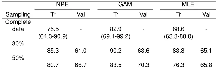
TABLE 2.1 : Serum sodium analysis: Complete data and mean AUCs (%) from 1000 resamples . . . 17

TABLE 3.1 : Correlation between density means and various lipoprotein particle biomark-ers. Abbreviations: HDL, high density lipoprotein; LDL, low density lipopro-tein; VLDL, very low density lipoprolipopro-tein; Tg, triglyceride; Tc, total choles-terol; LPIR, lipoprotein insulin resistance score; S, small; M, medium; LM, large-to-medium; L, large; VL, very large. CRP, C-reactive protein; IL-6, Interleukin 6. Suffixes: z, size; p, particle number; c, cholesterol concentra-tion.∗ρ×100are shown. . . 30

TABLE 4.1 : Simulation 1 results. M=500 for each simulation set, with N=300 per simula-tion. RMSE: root-mean-square error; AUC: area under ROC curve. . . 45 TABLE 4.2 : Simulation 2 results. M=500 for each simulation set, with N=300 per

LIST OF ILLUSTRATIONS

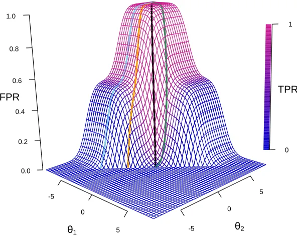
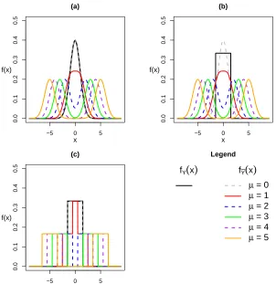
FIGURE 2.1 : Plot ofFPR(θ)andTPR(θ). TPR(θ)is the color overlay ofFPR(θ), repre-sented as the surface plot. The colored curves along the surface represent sample φ’s. The black curve represents the φof the optimal ROC. The corresponding ROC curves are shown in Figure 2.2. The plot represents underlying data densities in Figure 2.3a (µ= 2.5). . . 9 FIGURE 2.2 : ROC curves corresponding toφ’s in Fig 2.1. . . 10 FIGURE 2.3 : Simulation densities for XY and X_Y¯. (a) mixture of normals for f_Y¯(x)

and normal for fY(x); (b) mixture of normals for f_Y¯(x) and uniform for

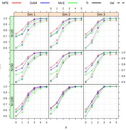
fY(x)uniform; (c) mixture of uniforms forf_Y¯(x)and uniform forfY(x). . . . 14 FIGURE 2.4 : Mean AUCs (%) from 1000 simulations from independent training (Tr) and

validation (Val) sets in simulations. . . 15 FIGURE 2.5 : ROC curve and φ. Solid and dashed lines represent the truth (the data

generating distributions shown in red and orange) and NPE of the ROC curve andφ. . . 16

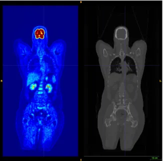
FIGURE 3.1 : Left: PET image. Intensity levels (shown in jet color spectrum) indicate the level of 18_{F-FDG uptake in tissue. Right: Corresponding CT image}

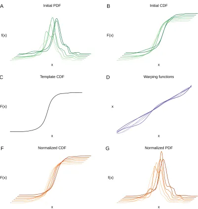
in grayscale. The anatomical structures are more pronounced, and the intensity levels indicate tissue density. . . 21 FIGURE 3.2 : Normalization workflow. Empirical densities fi(x)(A) are transformed to

Fi(x)(B). A template density Fm(x)(C) is chosen and warping functions

wi(x)(D) are estimated. Using a modified functional regression, normal-ized warping functions wnorm

i (x)are calculated, which are then used to estimate the normalized densitiesFnorm

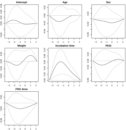
i (x)(E) andfinorm(x)(F). . . 26 FIGURE 3.3 : Coefficient functions of the restricted function-on-scalar regression using

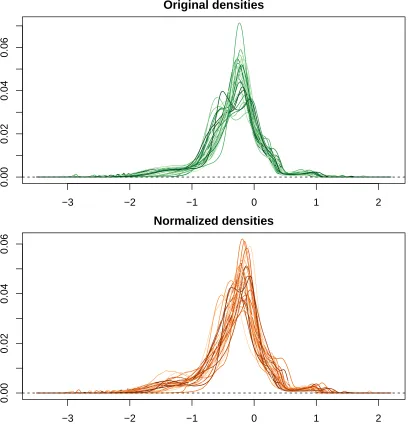
six covariates. . . 28 FIGURE 3.4 : Empirical densities of PET intensities of 32 baseline scans. The top curves

represent original densities, and the bottom represent densities after re-moving the effects of nuisance parameters. . . 29

FIGURE 4.1 : Trajectories by APOE risk category and overlay of proposed trajectories . 35 FIGURE 4.2 : Simulated data per simulation 1a. The color gradient indicates the

propor-tion of the subject being sampled as an accumulator. . . 39 FIGURE 4.3 : ADNI mean trajectories by APOE risk group. The red curve is the mean

CHAPTER 1

I

The field of biomedical imaging has transformed in recent decades from simple applications, such

as visualization of broken bones using projection radiographs, to vastly more complex applications,

such as quantification of brain activity using functional magnetic resonance imaging. Advances

in imaging technology has made it possible to observe real-time in vivo disease processes, e.g.

the level of impaired bone mineralization or the amyloid plaque burden in the brains of Alzheimer’s

disease (AD) patients, that until recently could only be seen post mortem or using invasive methods

such as biopsies. The transition from qualitative to quantitative applications in biomedical imaging,

along with increasing understanding of the relationship between various disease biomarkers and

clinical outcomes, has highlighted the importance of robust statistical methods.

This dissertation focuses on positron emission tomography (PET) and statistical methodologies

in-spired by problems encountered during the analysis of PET data. The motivation comes from the

Vascular Inflammation in Psoriasis (VIP) trial. The VIP trial is a multicenter, randomized controlled

trial to assess the effects of adalimumab, a biological systemic therapy, on systemic vascular

in-flammation in subjects diagnosed with moderate to severe psoriasis, as compared to narrow-band

ultraviolet B phototherapy or placebo. The primary outcome measure is the change in total

vascu-lar inflammation in aortic segments as assessed using18_{F-fludeoxyglucose (FDG) PET/computer}

tomography (CT) between baseline and end of study. The timing of the start of the dissertation

research coincided with the start of the VIP trial, and the opportunity naturally arose to observe and

participate in the analytic planning of the trial. This opportunity eventually evolved into the first two

chapters of this dissertation.

Chapter 2 is inspired by a novel application of FDG-PET/CT to quantify the level of skin

inflamma-tion. With the goal to quantify and correlate PET signals with clinical psoriasis severity measures,

skin segmentations need to be superimposed on the FDG-PET images that contain measures of

metabolic activity. A method for image segmentation, or the partitioning of an image into segments

of interest, is devised for the skin using the CT image, where a bivariate threshold (i.e. upper

Gaus-sian filter. This chapter addresses the performance assessment of bivariate thresholding such as

the interval classification used in the segmentation method. However, after the methodology was

developed, it was noticed that proper co-registration, or alignment, of PET image to the CT

segmen-tations became impossible due to significant movements of the extremities during image acquisition

in the VIP trial. A dataset from serum sodium levels in patients hospitalized for fulminant bacterial

meningitis fit the classification scenario was substituted as the motivating example.

While parallels can be drawn from the classic binary classification scenario and the receiver

op-erating characteristic (ROC) analysis, these classic approaches are inadequate and restrictive for

classification beyond simple univariate binary thresholding. Simple classification scenarios

involv-ing thresholdinvolv-ing a predictor usinvolv-ing a cutpoint offer straightforward assessments of classifier

perfor-mance using the ROC curve, but in complex scenarios, such as bivariate thresholding, the ROC

curve is not specified. Chapter 2 presents a generalization of the ROC analysis, introduces the

concept of the parameter path in the ROC space of a classification scenario, and defines the

opti-mal ROC (OROC) to identify and assess performance of optiopti-mal classifiers. Interval classification,

where a predictor is thresholded using two cutpoints, is used to illustrate the OROC estimation and

show that nonparametric estimation (NPE) procedure simultaneously produces the parameter path

of the optimal classifier. Alternative semiparametric and parametric methods for OROC

estima-tion are presented: the generalized additive model (GAM), and the maximum likelihood estimaestima-tion

(MLE) based on a profile likelihood. The performance of the NPE, GAM, and MLE in Monte Carlo

simulations and application to the serum sodium dataset are presented.

Chapter 3 covers image normalization, a major topic in quantitative PET. Image normalization is

widely viewed as an essential preprocessing step for quantitative analysis. While great

advance-ments have been made in normalization for magnetic resonance imaging (MRI), quantitative

analy-sis of positron emission tomography (PET) primarily involves the use of standardized uptake values

(SUV) which aim to account for major sources of nuisance variation. However, these units are

highly susceptible to variations in imaging protocol and physiology. A normalization method based

on the application of functional data analysis to image intensity distribution functions is proposed

in this chapter, with the assumption that individual density functions are variations from a template

regression, the variations in density functions due to nuisance parameters are estimated and

sub-sequently removed for normalization. This chapter outlines image intensity density normalization

and includes the application to the VIP trial dataset. Additionally, the normalized densities show

correlations with cardiovascular biomarkers that are not present in the original densities.

Chapter 4 presents another interesting PET data problem in the realm of neuroimaging. The

prob-lem presents itself in the form of a plot (Figure 4.1) of longitudinal measurements of amyloid-beta

(Aβ) in the brain, using florbetapir-PET. There are striking features that show 1) differences by

genotypes, 2) an outline of a common trajectory function, and 3) possible clustering of subjects

who many have significant delay in Aβ accumulation. Aβ is an important biomarker in AD, and

a general hypothesis exists regarding the functional form of its longitudinal trajectory. Surprisingly,

even with various hypotheses on the shape of Aβtrajectories, no studies have integrated this

knowl-edge in modeling Aβtrajectories, with most analyses instead relying on basic linear mixed effects

models. This chapter describes a new approach using nonlinear mixed effects framework to model

Aβtrajectories as measured by florbetapir-PET in a cohort of patients from the Alzheimer’s Disease

Neuroimaging Initiative (ADNI). The hypothesized functional form of Aβtrajectory is incorporated by

assuming 1) a common trajectory function for all subjects, with variations in the location parameter,

and 2) a mixture distribution for the random effects of the location parameter to address an

em-pirical findings that some subjects may not accumulate Aβ. Using a Bayesian hierarchical model,

group differences are specified into the trajectory parameters. Monte Carlo simulation results are

presented to show the performance of model estimates under various scenarios. Application to the

ADNI data show an estimated difference of 21 years in the onset of Aβbetween average and high

CHAPTER 2

E

ROC

2.1. Introduction

Assessment of classifier performance is well established for simple biomedical scenarios. The most

common methods quantify the tradeoff between correct and incorrect disease classifications to

de-termine the performance of a biomarker, and these methods are prevalent in binary classification

settings. While these methods may be sufficient for classification that involves thresholding a

con-tinuous score, they are not be able to accommodate complex classifications such as multivariate

thresholding. In the setting of multiple thresholds, the traditional single threshold method cannot

be used to assess the performance of the classifier. Alternatively, the performance measure of the

classifier must accurately reflect the classification rule.

The receiver operating characteristic (ROC) curve is the standard method of assessing classifier

performance, owing largely to the simplicity of its graphical and statistical interpretation (Metz,

1978; Pepe, 2003). The ROC curve is defined in the binary setting, where two distinct classes

are assumed to have different (i.e. separated) distributions of a common measure such that partial

separation of distributions can be achieved using a single cutoff. In this particular setting, the ROC

curve has been extensively characterized and its properties are well understood.

In the framework of the simple thresholding of a dependent variable that allows the tradeoff

be-tween sensitivity and specificity to be used, extensions have been developed for more complex

decision rules, with the emphasis primarily on ternary classification such as trichotomous

classi-fication (Dreiseitl, Ohno-Machado, and Binder, 2000; Mossman, 1999) and transitional (ordinal)

classification (Alonzo and Nakas, 2007; Nakas and Alonzo, 2007). These classifier assessment

methods rely on a seemingly natural extension of the ROC curve, the ROC surface, whose

volu-metric interpretation is similar to the area under the ROC curve (AUC) (Dreiseitl, Ohno-Machado,

and Binder, 2000; Mossman, 1999; Nakas and Yiannoutsos, 2004; Nakas and Alonzo, 2007).

However, traditional ROC analysis suffers the major limitation of an assumption of classification

such as biomedical image segmentation (i.e. classification of features of an image as anatomical or

disease classes) using a multimodal histogram where a feature of interest has values only within a

specific interval (Chen, 2008). A histogram of the image intensity values may assume a multimodal

distribution, and a segmentation algorithm may partition the histogram using thresholds based on

features such as valleys in the histogram. Another scenario to consider is predicting survival of

pa-tients based on biomarkers at admission to a hospital in papa-tients with fulminant bacterial meningitis

(Muralidharan, Mateen, and Rabinstein, 2014), where serum sodium level within a specific range

may predict survival better than using single threshold. In such cases, traditional ROC analysis,

which can only assess the sensitivity and specificity tradeoff for one threshold at a time, are no

longer useful.

We propose a simple generalization of ROC analysis that does not impose a binary cutoff restriction

and can easily accommodate various classification scenarios. In Section 2.2, we introduce optimal

ROC framework and apply this concept using a simple case that involves classification bounded

by two thresholds, or interval classification. We demonstrate nonparametric, semiparametric, and

parametric estimation procedures for the generalized ROC analysis, and show that the

nonpara-metric estimation procedure has the benefit of simultaneously estimating the optimal thresholds for

a given sensitivity or specificity. In Section 2.4, we compare the performance of the various

pro-posed ROC methods in simulation studies. In Section 2.5, we apply these methods to the study of

serum sodium levels for predicting survival in bacterial meningitis patients.

2.2. Description

2.2.1. Classical terminology

We adopt the traditional terminology from the simple binary classification scenario. The true class

membershipY ={1,0}is predicted using a continuous predictorX. For a given threshold

parame-terθ, an observation withX > θis classified asY = 1. Consequently, the true positive rate (TPR),

or sensitivity, is defined as the proportion of correctly classified positives (denoted asY):

The false positive rate (FPR), or 1-specificity, is defined as the proportion of incorrectly classified

negatives (denoted asY¯):

FPR(θ) =P(X > θ|Y = 0) =P(X_Y¯ > θ). (2.2)

While the plot ofTPRas a function ofFPR(θ)traditionally represents the ROC curve (Pepe, 2003),

we use a more general representation of the ROC as a vector-valued function,

ROC(θ) ={FPR(θ), TPR(θ)},forθ∈Θ. (2.3)

In traditional binary classification,Θ =R, and the plot is a monotonic curve. Specifically, the ROC

curve is a function of the data generating distribution, the classifier f, and its parameter θ. In

simple classification, the classifier is based on a single parameterθand it can be summarized as

an indicator function

f(θ, X) =I(X > θ). (2.4)

The performance of the classifier is summarized using the AUC by integratingTPRoverFPR.

2.2.2. Parameter path of the ROC curve and the optimal ROC

The tradeoff betweenTPR andFPRis graphically summarized by the ROC curve. In the simple

classification scenario,TPRas a function ofFPR(θ)is sufficient to describe the performance of the

classifier overΘas an ROC curve. In the more general case,θ∈Θmust be properly structured to

represent a classifier in ROC space.

For a classifierf, we define a continuous pathφ,

φ: (0,1)7→Θ, (2.5)

where lims→0φ(s) corresponds to (0,0) in the ROC plot, and lims→1φ(s) corresponds to (1,1).

In the simple classification case,lims→0φ(s) = −∞and lims→1φ(s) = ∞. Conceptually,φcan

be represented as a sequence of θ that plots the ROC curve from (0,0) to (1,1). We denote the

In a given classification schema,Φproduces set of all possible ROC curves. Since it is convention

to attribute one ROC curve to a classifier, from now we refer to φas a classifier. Revisiting the

ROC, it can now be defined as a function of the classifier and data:

ROC(F_Y,Y¯,φ, s) ={FPR(φ(s)), TPR(φ(s))}, s∈[0,1]. (2.6)

Furthermore, we generalize the AUC as the integration ofTPRoverφtransformed toFPR:

AU C=

Z

φ

TPR(θ)dFPR(θ)·dθ. (2.7a)

It can be reparameterized as an integral overFPR:

AU C=

Z 1

0

TPR(φ(s))dFPR(φ(s)). (2.7b)

In the case where FPR is an invertible function whose domain is φ(s), s ∈ [0,1], substituting

u=FPR(φ(s)), (2.7b) becomes more familiar:

AU C=

Z 1

0

TPR(FPR−1(u))du. (2.7c)

The concept of the optimal ROC is straightforward. For a given classification scenario inΦ, we are

interested in a classifierφthat achieves the best classification. Namely, we wantφthat achieves

the optimal ROC, with optimality defined by a feature (generally the AUC) of the ROC curve:

arg max

φ

AU C(φ) :={φ| ∀τ ∈Φ:AU C(τ)≤AU C(φ)}. (2.8)

In simple classification, {Im(φ)} ≡ R implicitly defines a unique φ that spans from −∞ to ∞,

therefore it is the optimal ROC classifier.

2.2.3. Interval classification

The concept of optimal ROC may seem trivial in simple classification, but its importance is

classification function defined as

f(θ, X) =I(θ1< X < θ2). (2.9)

We refer to this as interval classification, and the decision rule is also straightforward. In this case,

theTPRis:

TPR(θ) =P(XY > θ1∩XY < θ2). (2.10)

Similarly,FPRis defined as

FPR(θ) =P(XY¯ > θ1∩XY¯ < θ2). (2.11)

A contour plot ofFPR(θ)andTPR(θ)(Fig 2.1) best illustrates Θ, now a subset of R2_{, and Φ of}

this schema. As before, define a path represented as an arc along the surface with end points

parameterized as 0 and 1, respectively representing (FPR, TPR) of (0,0) and (1,1). Let φbe a

continuous function that maps the arc to the parameters that constitute an ROC curve, such that

lims→0φ(s) ={θ, θ}for someθ∈Randlims→1φ(s) ={−∞,∞}. In this scenario,Im(φ)is a set of

θ∈R2_{that defines an ROC curve. It is evident that a uniqueφdoes not exist; rather, many possible}

classifiers exist. The corresponding ROC curves of the fourφs highlighted in (Fig 2.2) show a wide

classifier performance range, butφ1has the largest AUC.

The AUC in interval classification has the following form:

AU C=

Z

φ

TPR(θ)dFPR(θ)dθ

=

Z

φ

P(XY ≥θ1∩XY ≤θ2)·

d{P(XY¯ ≥θ1∩XY¯ ≤θ2)}dθ.

The conventional interpretation of the AUC is the probability of correctly ordering diseased and

non-diseased in simple classification (Pepe, 2003). This interpretation is more difficult in complex

-5

0

θ1 5 0.0

-5

0

θ2 5

0 0.2

0.4

FPR

0.6 0.8 1.0

TPR

1

Figure 2.1: Plot ofFPR(θ)and TPR(θ). TPR(θ) is the color overlay ofFPR(θ), represented as the surface plot. The colored curves along the surface represent sample φ’s. The black curve represents theφof the optimal ROC. The corresponding ROC curves are shown in Figure 2.2. The plot represents underlying data densities in Figure 2.3a (µ= 2.5).

θ1=−θ2for all points alongφ, it can be easily seen that

AU C=P(|XY|<|X_Y¯|), (2.12)

which is similar to the probabilistic interpretation of AUC in the classical case.

2.3. OROC estimation

We present three methods for estimating the optimal ROC for our interval classification scenario,

0.0 0.2 0.4 0.6 0.8 1.0

0.0

0.2

0.4

0.6

0.8

1.0

FPR

TPR

2.3.1. Nonparametric estimation

Ideally, we want to estimate theφthat satisfies the definition of optimality (2.8) for a given

classi-fication scenario. From a random sample(X1, Y1), . . . ,(Xn, Yn), we may simultaneously estimate

theφand optimal ROC curve nonparametrically. Formally, for each possible value ofFPR=s, we

choose the parametersθthat have the correspondingFPRand maximumTPR:

b

φ_Opt(s) = arg max

θ:FPR(θ)=s

TPR(θ) :={θ| ∀π:TPR(π)≤TPR(θ)}. (2.13)

Monotonicity is guaranteed sinceFPR(θ1, θ2)≤FPR(θ1−δ1, θ2+δ2)andTPR(θ1, θ2)≤TPR(θ1−

δ1, θ2+δ2)for anyδ1, δ2 >0. φb_Opt(u)is the estimator forφin (2.8); maximization ofTPRover all

values ofFPRresults in maximizing the AUC. Alternatively, for a given value ofTPR=s, θcould

also be chosen to have the minimumFPR:

arg min

θ:TPR(θ)=s

FPR(θ) :={θ| ∀π:FPR(π)≥FPR(θ)}. (2.14)

The two methods are equivalent and yield the same optimal ROC curve, sinceTPRforθˆobtained

for given value ofFPRreturnsθˆby definition, and vice versa.

The nonparametric method simultaneously estimates the classifierφand the optimal ROC curve.

In the interval classification scenario,φis represented by a continuous path along the ROC surface

in Figure 2.1, butφmay include any set of discontinuous or disjointed paths that give rise to the

optimal ROC. From this point, we refer to the nonparametric optimal ROC classifier estimation as

NPE. Appendix A is the R code for nonparametric estimation of the optimal ROC AUC.

2.3.2. Semiparametric estimation

An alternative method for estimating the optimal ROC for the interval classification is a generalized

additive model (GAM) using quadratic penalized regression splines with smoothing parameters

se-lected by REML (Hall, Hyndman, and Fan, 2004; Hastie and Tibshirani, 1986) for the classification

of class membership. The model is simply

where the functionf is a smooth function ofX, modeled using thin plate regression splines (Wood,

2003). For interval classification, the general shape off is a smooth curve with a single hump

centered between the intervals and low values outside of the interval (e.g. a quadratic curve).

The performance assessment ofφis straightforward: the predicted value from (2.15) can be

thresh-olded as in the classical scenario, and a simple area under the ROC curve can be employed to

estimate the optimal ROC. Additionally,f−1_{{logit(ˆp)} ∈ {Im(φ}ˆ_{)}soφcan be estimated indirectly,}

and we refer to this semiparametrically estimated classifier as theGAM classifier. We implement

this using the R (R Core Team, 2014) package mcgv (Wood, 2000, 2004, 2011).

2.3.3. Parametric estimation

Another alternative method for optimal interval classification is specifying a parametric model. For

our interval classification scenario, we can incorporate the complex decision rule directly into a

generalized linear model and maximize the model likelihoodLunder

logit{Pr(Y = 1|S)}=α+βI(θ1< X < θ2). (2.16)

Our parameter of interest isθ={θ1, θ2}. We estimate{θ, α, β}using a profile likelihoodLθ( ˆαθ,βˆθ).

For eachθusing a grid search, we findαˆandβˆ. Subsequently, we evaluate

ˆ

θOpt= arg max

θ

Lθ( ˆαθ,βˆθ), (2.17)

which we refer to as theMLE classifier. We assess the performance of the MLE classifier using

ROC curve generated from the logistic model or direct classification.

2.4. Simulation

To compare the proposed estimation techniques for the optimal ROC, we simulate from

data-generating distributions consistent with the interval threshold setting, where XY is sandwiched

byXY¯. We first consider symmetric distributions for simplicity using bimixture distributions, and we

then consider estimatingφusing asymmetric distributions. The data are independently generated

2.4.1. Simulation - symmetric distributions

Three different scenarios are considered for our simulations, with variations in distributional overlap

betweenXY andX_Y¯. In the world simulation, we use a normal distribution and a mixture distribution

of normals (Figure 2.3a). For each observationsi= 1, ..., N, we randomly sampleXY i ∼ N(0,1),

and for each observationsi =N+ 1, ...,2N, we randomly sampleX_{Y i}¯ ∼ 1₂N(−µ,1) + 1₂N(µ,1).

In the second simulation, the distribution of the score for cases is modified to a uniform distribution

(Figure 2.3b). For each observations i = 1, ..., N, we randomly sampleXY i ∼ U nif(−1.5,1.5),

and for each observationsi =N+ 1, ...,2N, we randomly sampleXY i¯ ∼ 12N(−µ,1) + 1

2N(µ,1).

The third simulation involves a biuniform distribution flanking a uniform distribution (Figure 2.3c);

the distributional overlap is no longer transitional. For each observationsi= 1, ..., N, we randomly

sampleXY i∼U nif(−1.5,1.5), and for each observationsi=N+ 1, ...,2N, we randomly sample

X_{Y i}¯ ∼ 1₂U nif(−µ−1.5,−µ+ 1.5) + 1₂U nif(µ−1.5, µ+ 1.5).

2.4.2. Simulation results

We simulateB = 1000datasets for each parameter combination and obtained AUC performance

measures for the training and validation sets. Figure 2.4 summarizes the mean AUCs. In all

simu-lations, the AUC increases with greater separation betweenXY andXY¯ (i.e. increasingµ).

While there is a tendency for the NPE to overfit the data when the separation is small (i.e. greater

overlap between XY and X_Y¯), more so than the GAM and the MLE, the NPE performs better

than GAM and MLE in small sample sizes and smaller separations in distributions. With sharp

distributions (i.e. uniform, simulations 2 and 3 in Fig 2.4), the NPE once again performs better than

GAM and MLE in smaller sample sizes and separations. In general, the optimal ROCs from NPE

and GAM methods are more similar than those of the MLE method, and this may be attributed to

the estimation of a single point in the MLEφ.

2.4.3. φestimation

Figure 2.5 illustrates the NPE of φ. We simulated data using asymmetric distributions with the

following parameters: XY i ∼ N(1,1), XY i¯ ∼ 12N(−0.5,1) + 1

2N(2,1), andN = 500each forXY

−5 0 5

0.0

0.1

0.2

0.3

0.4

0.5

(a)

f(x)

x

−5 0 5

0.0

0.1

0.2

0.3

0.4

0.5

(b)

f(x)

x

−5 0 5

0.0

0.1

0.2

0.3

0.4

0.5

(c)

f(x)

x

Legend

fY

(

)

(

)

µ = 0

µ = 1

µ = 2

µ = 3

µ = 4

µ = 5

Figure 2.3: Simulation densities forXY andX_Y¯. (a) mixture of normals forf_Y¯(x)and normal for

fY(x); (b) mixture of normals forf_Y¯(x)and uniform for fY(x)uniform; (c) mixture of uniforms for

µ A UC 0.5 0.6 0.7 0.8 0.9 1.0

0 1 2 3 4 5

● ● ● ● ● ● ● ● ● ● ● ● ● ● ● ● ● ● ● ● ● ● ● ● ● ● ● ● ● ● ● ● ● ● ● ● Sim 1 N=100 ● ● ● ● ● ● ● ● ● ● ● ● ● ● ● ● ● ● ● ● ● ● ● ● ● ● ● ● ● ● ● ● ● ● ● ● Sim 2 N=100

0 1 2 3 4 5

● ● ● ● ● ● ● ● ● ● ● ● ● ● ● ● ● ● ● ● ● ● ● ● ● ● ● ● ● ● ● ● ● ● ● ● Sim 3 N=100 ● ● ● ● ● ● ● ● ● ● ● ● ● ● ● ● ● ● ● ● ● ● ● ● ● ● ● ● ● ● ● ● ● ● ● ● Sim 1 N=50 ● ● ● ● ● ● ● ● ● ● ● ● ● ● ● ● ● ● ● ● ● ● ● ● ● ● ● ● ● ● ● ● ● ● ● ● Sim 2 N=50 0.5 0.6 0.7 0.8 0.9 1.0 ● ● ● ● ● ● ● ● ● ● ● ● ● ● ● ● ● ● ● ● ● ● ● ● ● ● ● ● ● ● ● ● ● ● ● ● Sim 3 N=50 0.5 0.6 0.7 0.8 0.9 1.0 ● ● ● ● ● ● ● ● ● ● ● ● ● ● ● ● ● ● ● ● ● ● ● ● ● ● ● ● ● ● ● ● ● ● ● ● Sim 1 N=20

0 1 2 3 4 5

● ● ● ● ● ● ● ● ● ● ● ● ● ● ● ● ● ● ● ● ● ● ● ● ● ● ● ● ● ● ● ● ● ● ● ● Sim 2 N=20 ● ● ● ● ● ● ● ● ● ● ● ● ● ● ● ● ● ● ● ● ● ● ● ● ● ● ● ● ● ● ● ● ● ● ● ● Sim 3 N=20

NPE GAM MLE Tr Val

0.0 0.2 0.4 0.6 0.8 1.0

0.0

0.2

0.4

0.6

0.8

1.0

FPR TPR

−2 0 2 4

X

.4 .2 0

f(x)

ROC t2

t1

fY(x) fY(x) estm.

Figure 2.5: ROC curve andφ. Solid and dashed lines represent the truth (the data generating distributions shown in red and orange) and NPE of the ROC curve andφ.

The NPE ROC curve is remarkably close to the true optimal ROC curve. There is expected noise

inφb, especially at the beginning of the ROC curve, but the overall path is captured. The intervals

betweenθ1andθ2in the true and estimatedφare consistent over the values of FPR.

2.5. Serum sodium data

The motivating dataset is from a retrospective study that sought to identify neurological factors

associated with poor outcome in adult patients with fulminant bacterial meningitis (Muralidharan,

Mateen, and Rabinstein, 2014). Serum sodium at admission was obtained in 39 patients

hospi-talized for fulminant bacterial meningitis at the Mayo Clinic in Rochester, Minnesota. The primary

end-point of the study was in-hospital mortality.

higher risk of poor outcomes (i.e. death) (Kratz et al., 2004), whereas serum sodium levels inside

the ideal range would carry no additional risk of death. With the outcome defined as survival,

we estimate the OROC using the NPE method and compare it with the GAM and MLE methods.

Table 2.1 contains the complete data analyses along with bootstrapped 95% confidence intervals

(n= 1000).

Although the GAM has the highest AUC at 0.83, it was not significantly different from the NPE and

MLE methods (AUCs of 0.76 and 0.69, respectively). It is possible that due to a small sample size,

outliers may force the flexible splines of the GAM to estimate a functional form that is cubic instead

of quadratic in nature, thereby losing the fidelity to the classification decision rule. We also assess

the performance of the different classifiers using subsampling at random at 30% and 50% of the

observed sample size which shows with similar cross-validated results.

NPE GAM MLE

Sampling Tr Val Tr Val Tr Val

Complete

data 75.5 - 82.9 - 68.6

-(64.3-90.9) (69.1-99.2) (63.3-88.0) 30%

85.3 61.0 90.2 63.6 83.3 65.1 50%

80.7 66.7 83.5 70.3 76.3 65.8

Table 2.1: Serum sodium analysis: Complete data and mean AUCs (%) from 1000 resamples

2.6. Discussion

We generalize ROC-based performance assessment in complex classification settings by defining

a classifier φ as a path in the ROC space. The example of interval thresholding illustrates the

inherent limitations of applying the traditional binary decision rules associated with ROC curves,

and the OROC offers an easy and intuitive framework to assess performance of interval classifiers.

Unlike the MLE classifier, where only a single classification table can be obtained, the NPE and

GAM classifiers have flexibility in range of classification statistics. The NPE classifier, however, has

the advantage of ease of interpretation; the directly estimatedφplotted over the ROC curve such

in Figure 2.5 provides an intuitive look-up table for the classifier, and simple comparisons of new

may improve estimation ofφ.

While GAM has the added benefit of natural accommodation of external covariates, which can be

useful in applications such as tissue segmentation described above, existing methods for

covariate-adjusted ROC analysis (Janes and Pepe, 2009) may be applicable to the NPE. Furthermore, the

flexibility of the GAM may make it susceptible to influential outliers. This may result in loss of fidelity

to an a priori classification rule, whereas the NPE and MLE methods are bound by the

classifi-cation rule. Regarding comparison of NPE classifiers, existing tests using bootstrap estimates of

standard errors of the AUCs can be easily performed (Hanley and McNeil, 1982) without being

computationally expensive. Further work is necessary to investigate the asymptotic distribution of

the NPE AUC with and without distributional assumptions.

In addition to improvements in classification performance in data scenarios described in this

chap-ter, the simplicity of the performance measure of complex classifiers should make the application

of NPE and GAM more compelling. The present work uses the bivariate classification setting

ex-ample, but this methodology may be extended to multiple input scoresX1, X2, X3, ...and threshold

parameters θ1,θ2,θ3, .... Another interval thresholding scenario, albeit theoretical, may include

multimodal thresholding, e.g. I(tl1 < S < tu1∪ tl2 < S < tu2∪ ...), where clusters of intervals for

CHAPTER 3

I

N

PET

D

W

R

3.1. Introduction

Biomedical imaging modalities such as magnetic resonance imaging (MRI), computer tomography

(CT), and positron emission tomography (PET) are established cornerstones of qualitative

diag-nostics that allow visualization of structures and physiological function in healthy and diseased

subjects. Statistics have gradually transformed the use medical imaging from a qualitative to a

quantitative tool, allowing greater discrimination and more comprehensive descriptions of disease

status and prognosis. However, quantitative analysis of biomedical images is challenging due to

the many sources of unwanted variation that confound the signal. These sources range from

ma-chine calibration and scan parameters to the patient’s metabolic rate affected by ambient conditions

(Coxson, 2013). Without comparability of measurements, formal statistical inference suffers from

diminished power and potentially strong biases.

Image intensity normalization is generally acknowledged as a key preprocessing step in the

an-alytical pipeline. Various methods exist in the literature, including histogram matching (Nyul and

Udupa, 1999) and intensity normalization with respect to particular regions of interest (ROI)

(Shino-hara et al., 2014). In the latter example where particular anatomical structures are assumed to have

similar physical consistency, such as the normal appearing white matter or cerebellar gray matter

in the brain, simple z-score statistical normalization successfully removes a significant amount of

nuisance variability due to parameters such as scanner and platform. More often than not, these

benefits are conferred to imaging modalities with high resolutions (e.g. MRI) and well

character-ized tissue properties (e.g. density). In PET imaging, image resolution is bounded by an inherent

uncertainty of the radionuclide tracer location, image reconstruction is dependent on near-perfect

alignment of a reference image, and tissue-specific intensity is dependent on pharmacokinetics

and physiological state of the body. The standardized uptake value (SUV), a relative measure of

tracer uptake, compensates for the largest sources of signal variation, which include the amount

of injected tracer, patient body weight, and radioactive decay. Summary measures of SUV and

SUV in reference tissues, are mainstays in quantitative PET. Increasingly, however, it is becoming

clear that existing normalization methods for PET may be inadequate to handle these sources of

variability (Huet et al., 2015; Keyes, 1995).

In this chapter, we propose a new statistical normalization strategy based on the application of

functional data analysis (FDA) to image intensity distribution functions. FDA has been previously

proposed for analyzing densities by treating empirical density curves as functional data (FD) objects

(Alois Kneip, 2001) and conducting unsupervised analyses to investigate unwanted variation. One

such method directly uses the empirical probability density functions (PDF) as FD objects

(Deli-cado, 2011). Unfortunately, these normalizations suffer from undesirable properties, including the

violation of regularity conditions of the Hilbert space-based methods when applied to density

func-tions (Petersen and Mller, 2016). Outside of image analysis, supervised methods for normalization

using functional data have been proposed, such as functional normalization (funnorm) by Fortin et

al. (Fortin et al., 2014). This method uses simple additive models for quantile functions as FD

ob-jects. Unfortunately, coefficients near boundary values (i.e. at 0 and 1) may be subject to increased

uncertainty in estimation when studying quantile functions. The funnorm approach also does not

account for smoothness in the curves, but rather focuses on pointwise regression techniques in the

context of gene expression distributions. We propose a novel FDA approach to density-valued data

that uses a modified function-on-scalar regression applied to image-specific warping functions from

a template density function. This method aims to increase the flexibility to capture more shape

vari-ation and reduce estimvari-ation uncertainty at boundary limits, while maintaining interpretability and

improving statistical power for detecting group differences.

Our motivating example comes from the Vascular Inflammation in Psoriasis (VIP) Trial, a

random-ized, placebo-controlled study designed to test the effect of systemic therapy for psoriasis on

sys-temic vascular inflammation as measured by PET/CT. Psoriasis is a common inflammatory disease

that prominently manifests in the skin, but it is also independently associated with many

cardio-vascular comorbidities. These include myocardial infarctions (MI), stroke, and cardiocardio-vascular death

(Gelfand et al., 2006; Ogdie et al., 2015). The underlying inflammatory mechanism in psoriasis

is shared by other diseases that are associated with cardiovascular burden, and lowering

Figure 3.1: Left: PET image. Intensity levels (shown in jet color spectrum) indicate the level of

18_{F-FDG uptake in tissue. Right: Corresponding CT image in grayscale. The anatomical structures}

are more pronounced, and the intensity levels indicate tissue density.

glucose-analogue,18F-fludeoxyglucose (FDG), may be used as a biomarker to measure the level

of metabolic activity. Figure 3.1 is a coronal (frontal) plane image view of a PET/CT scan of a

study patient; red regions, including the brain, show tissue with high18_{F-FDG uptake, indicative of}

high metabolic activity. Our goal in this work is to improve quantification of systemic inflammation

through improved normalization of the PET image. In the remainder of this chapter, we apply our

normalization to the VIP data and compare the correlation between densities and cardiovascular

3.2. Methods

3.2.1. Density-valued data

In PET, the raw unit of measure is radioactivity concentration of becquerels per cubic centimeter

(Bq/cc). This unit reflects the amount of radionuclide tracer concentration (i.e.18_{F-FDG) in tissue,}

and is the quantitative unit for a given voxel in a PET scan image. We denote the intensity at a given

voxelvasY(v), which arises from an intensity distributionf. We make fundamental assumptions of

the data that the intensity distribution of a scan for a patient is a realization of a stochastic process

that generates these distributions. We further assume that the variations from a template density

fmare attributable to biological and non-biological factors, and can be modeled statistically.

3.2.2. Warping functions

For each subjecti, we define the density-valued image intensity data as the empirical probability

density function fi(x), where x represents image intensity values and ranges. Likewise, we let

Fi(x)represent corresponding cumulative distribution function. We denote the population template

function byFm(x) = Rx

0 fm(u)du, and define the warping functionwi(x)as the function that maps

Fm(x)toFi(x). That is, a warping functionwiremaps the domain such that

Fm{wi(x)}=Fi(x). (3.1)

The warping function is represented as a curve, with the identity functionwI(x) =xindicating no

warping. To define the template function, we use the depth measure of centrality of a given curve

within a group of curves as defined by Fraiman and Muniz (2001). We use the functional median

of a set of curves, which is defined as the functionFm(x)having the greatest integrated depth.To

assess the systematic effects of sources of variation that are not related to the biological processes

of interest, we next propose to study the warping functions using functional regression models.

3.2.3. Restricted function-on-scalar regression

Following the assumption that the variations from the population mean or template intensity

of observed variables that are not of interest for the study; for example, the dose of radionuclide

tracer administered only introduces unwanted variation into the measurements. We further denote

byXi= (Xik)Kk=1the vector predictors of interest for subjecti. Since CDFs range from 0 to 1, the

warping functions at domain boundaries are restricted to the identity functions. This can be further

simplified by subtracting thewI(x)fromwi(x)to yield functional responsesri(x)that are restricted

to 0 at the domain boundaries.

Theri(x)can be modeled as functional responses for regression models with scalar predictors (i.e.

biological and non-biological factors). We employ regression models for functional responses and

scalar predictors (Ramsay, 2005; Reiss, Huang, and Mennes, 2010):

r(x) =Zβ(x) +(x). (3.2)

In this scenario, xranges over some finite interval X ⊂ R, and r(x) can be represented as an

N-dimensional functional response vector. The design matrixZ = [X V]isN ×qdimensional,

β(x) = [β1(x), . . . , βq(x)]Tis the functional coefficients vector, and(x)is the functional error vector.

Consider the b-spline basis function representation ofr(x),

r(x) =Cθ(x), (3.3)

whereθ(x) = [θ1, . . . , θK]T]is the vector ofKb-spline functions andC is anN×Kmatrix of basis

coefficients. The coefficient functions in (3.2) are then represented as

βk(x) =bkθ(x), (3.4)

wherebkis the basis coefficient vector. The problem reduces to estimatingB= (b1, . . . ,bq)T _using

this general form of (3.2):

r(x) =ZBθ(x) +(x). (3.5)

However, for the warping functions to yield proper CDFs, the aforementioned restriction tor(x)must

be implemented. The basis function representation in (3.3) offers a simple solution to implement

last b-spline basis components:

B∗N×(K−2)=BN×K×      

0K−2

IK−2

0K−2

     

K×(K−2)

, (3.6)

and

θ∗(x) = [θ2, . . . , θK−1]T. (3.7)

We estimateB∗by minimizing the following:

Z

kCθ(x)−ZB∗θ∗(x)k2_dt+ q X

k=1

λk Z

[L(b∗_kθ∗(x))]2dt. (3.8)

The second term is a roughness penalty with a non-negative tuning parameter λ and a linear

differential operatorL. We use a second derivative operator forL.

Since the basis functionsθ1andθK only contribute to the functional range at the boundaries ofX,

we first estimateB∗ and then add the zero coefficients, i.e. Bˆ = [0K Bˆ

∗

0K]. We calculate the

estimates of coefficient functionsβ_k(x)and their standard errors fromBˆusing standard methods

penalized likelihood estimatingλusing generalized cross-validation. We implement the restricted

function-on-scalar regression (rfosr) with the aforementioned modifications to the fosr function (Reiss, Huang, and Mennes, 2010) in therefundpackage for R (Huang et al., 2015). Appendix B is the R code forrfosr.

3.2.4. Normalization

We assume that the degree to which an intensity distribution of a particular scan differs from the

population template is captured by the warping functions, and that the modeled estimated

coef-ficient for various factors are additive in nature and can be adjusted for. Our overall approach to

normalization is to regress out the effects of nuisance factors from the warping parameters, and

ulti-mately estimate an intensity distributionFnorm

i (x)adjusted for the nuisance factors for each image.

Using functional regression, we separate Zand β(x)to K predictors of interest andJ nuisance

We form the normalized functions,

ˆ

rnorm(x) =r(x)−VJβˆJ(x), (3.10)

which we use to form the normalized warping function functionswˆnorm(x). Following the warping

function representation (3.1), the we normalize distributions using the normalized warping

func-tions:

ˆ

F_inorm(x) =Fm{winorm(x)} (3.11)

Figure 3.2 illustrates the normalization procedure. First, we convert empirical densitiesfi(x)(A)

toFi(x)(B). We choose a templateFm(x)(C) and calculate warping functionswi(x)(D). We then

regress out the nuisance effects on the warping functions and estimate the normalized warping

functionswnorm

i (x)to obtain the normalized density estimatesFˆinorm(x)(E) andf˜inorm(x)(F).

3.3. VIP Trial data

3.3.1. Motivating Study

As a proof of concept, we apply our normalization to the VIP Trial PET/CT imaging data and assess

sensitivity to associations between metabolic activity and lipoprotein particle biomarkers known to

be associated with cardiovascular risk (Austin et al., 1988; Gordon et al., 1989). We study the PET

scans, with intensities recorded in standardized uptake values (SUV), defined voxel-wise as

SU V(v) = I(v)

C/W (3.12)

whereI(v)is the PET scan and W is the weight of the patient. C is the corrected radionuclide

tracer activity, calculated as

C=T·2−

tS−tI t_{1/2 ,}

(3.13)

whereT is the injected tracer activity,tS is the time of scan,tI is the time of tracer injection, and

t1/2is the half life. Base 10 logarithm transformation of SUVs are used as primary units due to the

highly skewed distributions of the whole-body voxel SUVs.

●

A

x f(x)

Initial PDF

●

B

x F(x)

Initial CDF

C

x F(x)

Template CDF _D

x x

Warping functions

●

F

x F(x)

Normalized CDF

●

G

x f(x)

Normalized PDF

Figure 3.2: Normalization workflow. Empirical densitiesfi(x)(A) are transformed toFi(x)(B). A template density Fm(x) (C) is chosen and warping functions wi(x) (D) are estimated. Using a modified functional regression, normalized warping functionswnorm

i (x)are calculated, which are then used to estimate the normalized densitiesFnorm

single-pass full-body scans are not available for many subjects and instead the torso and lower

extremities are often scanned separately. To standardize the scanning protocol, we use

single-pass PET/CT scans and truncate at the same anatomic landmark for each scan (the femoral head).

Additionally, to eliminate scanner variability, we analyze scans from a single facility at the Hospital

of the University of Pennsylvania. We obtain log SUV densities after removing background using

active contour segmentation of tissue in ITK-SNAP (Yushkevich et al., 2006).

For the model, we choose variables that are known contributors to SUV variability, such as weight,

drug incubation time (i.e.tS −tI), and radionuclide dose (Boellaard, 2009), as well as plausible

biological factors such as age and sex. Since the underlying disease process is understood to be

associated with systemic metabolic activity and thus disease, we also included the psoriasis area

severity index (PASI), a clinical measure of psoriasis severity, in the model but do not residualize

based on PASI during normalization. Finally, we compare the SUV means before and after

normal-ization, and correlate the means with lipid and inflammatory biomarkers using each density’s mean

as a coarse measure of total systemic inflammation.

3.3.2. Results

Figure 3.3 shows the estimated functional coefficients of the covariates on wi(x), and figure 3.4

shows the densities before and after normalization (N=32). Of the six scalar covariates in the

model, incubation time has the greatest effect on the warping function, whereas FDG dose has the

least effect on the warping function.

Table 3.1 summarizes the association between the SUV density means and biomarkers pre- and

post-normalization (N=30). We use spearman’sρas a measure of correlation. None of the original

density means are statistically associated with the various lipoprotein and inflammatory biomarkers.

Employing the proposed normalization, we find LDL cholesterol concentration (LDLc), LDL particle

size (LDLp), very large LDL particle size (vl LDLp), total cholesterol (Tc), and IL-6 to be statistically

significantly associated density means.

3.4. Discussion

func-−3 −2 −1 0 1 2 −0.04 0.00 0.02 0.04 0.06 Intercept Coefficient function

−3 −2 −1 0 1 2

−0.04 −0.02 0.00 0.02 Age Coefficient function

−3 −2 −1 0 1 2

−0.06

−0.02

0.02

Sex

Coefficient function

−3 −2 −1 0 1 2

−0.04 −0.02 0.00 0.02 Weight Coefficient function

−3 −2 −1 0 1 2

0.00 0.02 0.04 0.06 0.08 0.10 Incubation time Coefficient function

−3 −2 −1 0 1 2

−0.06 −0.02 0.00 0.02 PASI Coefficient function

−3 −2 −1 0 1 2

−0.06

−0.02

0.02

FDG dose

Coefficient function

−3 −2 −1 0 1 2

0.00

0.02

0.04

0.06

Original densities

time

v

alue

−3 −2 −1 0 1 2

0.00

0.02

0.04

0.06

Normalized densities

v

alues

Original Normalized Biomarker ρ∗ p-value ρ∗ p-value HDLc 17 0.38 10 0.61 HDLp 3 0.87 -1 0.97

HDLz 3 0.89 0 1.00

S HDLp -23 0.22 -22 0.23 M HDLp 10 0.59 8 0.66 LM HDLp 16 0.40 13 0.49 L HDLp 20 0.30 16 0.39 IDLp -11 0.55 9 0.63

LDLc 16 0.40 44 0.02

LDLp 10 0.59 46 0.01

LDLz 20 0.29 2 0.91 S LDLp -1 0.94 29 0.11 L LDLp 31 0.10 28 0.13

VL LDLp 8 0.68 44 0.01

VLDLp -23 0.22 1 0.97 VLDLz -0.00 0.99 22 0.25 S VLDLp -32 0.08 -22 0.24 M VLDLp -9 0.62 17 0.37 LM VLDLp -11 0.56 17 0.37 L VLDLp -9 0.64 8 0.68 VLDLtg -15 0.43 12 0.53 Efflux value 20 0.31 13 0.52 Tg -14 0.47 16 0.41

Tc 16 0.40 39 0.03

LPIR -2 0.92 17 0.37 CRP -9 0.62 -6 0.77

IL-6 -30 0.10 -37 0.05

Table 3.1: Correlation between density means and various lipoprotein particle biomarkers. Abbrevi-ations: HDL, high density lipoprotein; LDL, low density lipoprotein; VLDL, very low density lipopro-tein; Tg, triglyceride; Tc, total cholesterol; LPIR, lipoprotein insulin resistance score; S, small; M, medium; LM, large-to-medium; L, large; VL, very large. CRP, C-reactive protein; IL-6, Interleukin 6. Suffixes: z, size; p, particle number; c, cholesterol concentration. ∗_{ρ×100are shown.}

functions of nuisance imaging protocol parameters and removes their effect. By modifying the

b-spline functional basis, we restrict the warping functions to yield proper density functions for

nor-malization. One of the strengths of our method is that it allows the use of full scan intensity densities

instead of using tissue-specific densities. Additionally, since we normalize the entire densities, the

use of reference tissues is not required.

Our application to the VIP Trial data shows promise that normalization may reveal signals that may

variability. The regression model indicates that the standardization using the SUV did not

ade-quately “standardize” the effects of the imaging parameters, in particular the FDG incubation time.

Increases in SUV have been noted with increases in FDG incubation time (Basu et al., 2007), with

standardizing the scan initiation time suggested as a corrective measure. In multi-site studies, these

corrective measures such as these may fall short due to the complex nature of PET/CT acquisition

and a statistical normalization may offer the best standardization.

While we have assessed our normalization in terms of association of the density means to

lipopro-tein biomarkers, another indicator for the usefulness of normalization would be to assess the

pri-mary outcomes of the VIP Trial, which are mean PET signals in the aorta. The density means

may offer a measure of cardiovascular risk via systemic inflammation, but they may also

oversim-plify the relationship between metabolic activity of the entire body and an inflammatory disease

process. Targeted quantification of the aorta using manual segmentations directly assesses the

atherosclerotic burden, and the use of normalized images, i.e. applyingwnorm

i and usingYnorm(v),

has the potential to improve dose-response and/or treatment effect signals. It is noteworthy,

how-ever, that LDL cholesterol concentration and particle size, which are associated with cardiovascular

disease (Sacks and Campos, 2003), are correlated with normalized density means. Our findings

are suggestive of stronger whole-body FDG signal throughout the body in patients with unhealthy

lipoprotein profiles. The significance of the weak inverse correlation of IL-6 and whole-body FDG

signal remains unclear, as IL-6 is implicated in pro- and anti-inflammatory processes (Scheller et

al., 2011).

The overall goals of normalization should be the comparability of quantitative imaging units for

population-level analysis, and the statistical principles of image normalization (Shinohara et al.,

2014) provide guidelines for image normalization. Although the proposed methodology is

theoreti-cally consistent with these principles, further work is required to empiritheoreti-cally assess the conformity

of our normalization process to these guidelines in large multi-center studies. Some assessments

are straightforward, such as testing the monotonicity of warping functions to assess the intensity

rank preservation. Preserving a similar distributions for similar tissues of interest may be more

challenging when a disease process may affect the distributions of every tissue class, such as the

systemic inflammatory process associated with psoriasis. Future extensions of our work will be

may affect the signal densities. Disentangling treatment effects in a tissue of interest from its effect

on the overall scan is paramount, and functional mixed effect-based models may be appropriate for

CHAPTER 4

N

-

β

PET

4.1. Introduction

Alzheimer’s disease (AD) is a neurodegenerative disease characterized by progressive

demen-tia unrelated to normal aging. The disease onset, or time of first symptoms, varies from person

to person, but the the disease progression is consistently characterized by accumulation of

amy-loid plaques in extracellular space between neurons and neurofibrillary tangles inside neurons. It

is believed that these characteristic structural features disrupt normal brain function and lead to

loss of neurons. Of interest is how these physical changes in the brain progress over time and

correlate with progression of disease. Accurately measuring amyloid-beta (Aβ) protein levels, the

components of amyloid plaques, is important in understanding the plaque burden as well as stage

of disease progression. In-vivo imaging of these structures may enable earlier AD diagnosis and

guide therapeutic regimens.

There is strong evidence that AβPET imaging is a promising biomarker of brain Aβ-plaque load

(Kepe et al., 2013). Currently there are two PET imaging compounds for Aβ: 1)

Pittsburgh-compound B (PiB) (Klunk et al., 2004), and 2) florbetapir (Clark et al., 2011), and both

radionu-clide tracers bind to Aβplaques in the brain. While PET applications using PiB has been around

since the early 2000’s, the more recent florbetapir has a favorable half-life profile (109.8 min in18F

florbetapir compared to 20.38 min in11_{C PiB), which allows an easier imaging protocol.}

Several trajectory shapes of major AD biomarkers have been theorized, and they generally are

based on the sigmoidal model (Caroli and Frisoni, 2010; Jack et al., 2010). However, their use

in charactering Aβ PET biomarker trajectories is limited; linear mixed effects (LME) models are

generally the basis of longitudinal trajectory modeling (Jack et al., 2012; Resnick et al., 2010,

2015). In the context of a sigmoidal trajectory model, the obvious limitation of LME model is the

nonlinearity of the hypothesized trajectory; linearity is assumed once a threshold is reached (i.e.

accounted for.

In this chapter, we propose a new method of modeling the Aβtrajectories based on a couple of

biological assumptions. The first assumption is that each subject has a unique Aβtrajectory based

on a common functional form (i.e. sigmoidal curve). The second assumption is that there are

sub-jects for whom the accumulation is not observed. In Section 4.2, we incorporate these assumptions

by combining a nonlinear mixed model framework with mixture of heterogeneous populations, and

formulate the trajectory model in a Bayesian framework. In Section 4.3, we evaluate the

perfor-mance of the Bayesian model in estimating the parameters using Monte Carlo simulation studies.

In Section 4.4, we apply these methods to the florbetapir dataset from the Alzheimer’s Disease

Neuroimaging Initiative (ADNI) cohort for estimating group differences in Aβtrajectories.

4.1.1. ADNI data

The Alzheimer’s Disease Neuroimaging Initiative (ADNI) is a consortium of researchers whose goal

is to collect, validate, and utilize study data to define the progression of AD. MRI and PET study

data are used, in addition to genetics, cognitive tests, and CSF/blood biomarkers, to understand

and predict AD. Florbetapir PET imaging has been collected in a cohort of subjects with ADNI,

which is publicly available (adni.loni.usc.edu).

The unit of Aβ florbetapir measure is the standardized uptake value ratio (SUVR), which is the

nonweighted SUV average across four main cortical regions (frontal, anterior/poster cingulate,

lat-eral parietal, latlat-eral temporal) divided by the SUV average across the composite reference region

(whole cerebellum, brainstem/pons, and eroded subcortical white matter) (Landau et al., 2015).

Figure 4.1 is a spaghetti plot of the Aβtrajectories in the ADNI cohort as measured by PET

imag-ing. To illustrate genetic differences, four color groups indicate the different AD risk profiles based

on APOE gene alleles. Typically, there are two to three Aβ measurements per subject, with an

average time between subsequent scans being 2 years. Due to radiation toxicity and cost of scans,