Using Quantitative Analytical
Techniques When Researching Real
Estate – Applied Example
Gary Garner
Lincoln University, New Zealand March 2012
Introduction
The acquisition of live data through case study analysis and subsequent application of econometric modelling techniques can often prove effective in the pursuit to explain trends in real estate values, despite characteristically limited availability of data sets (observations) especially in the case of larger property developments. Both linear and non-linear (polynomial and other forms) regression analysis techniques are typically utilised for this purpose. Such regression models describe and evaluate the relationship between a dependant variable , and other variables (independent variables ).
Overview
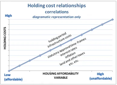
Regression techniques can be used for example, to establish the extent of the relationship between holding costs and housing affordability (and by implication, mortgage stress), by looking at a range of explanatory variables in holding cost components (i.e. independent variables) such as interest rates, inflation, and time frames for statutory approvals and overall holding period (Garner, 2012). This is schematically represented by Figure 1.
Measuring the sensitivity of the independent variable to holding costs can achieved by measuring the slope of the equation for incrementally increasing, or decreasing values. The trend / slope of the arctangent (measured in degrees) is measured and compared against arctangents for other variables that have been increased or decreased at the exact same increments (percentages). This process is sufficient to provide indicative levels of sensitivity based on the steepness of the angle, i.e. this comparison assists in the determination of which variables holding costs are most responsive to, e.g. interest, or development time, or undeveloped land cost, etc..
possible to measure their impact upon housing affordability since we can convert the holding cost outcome into a mortgage repayment equivalency expressed as a proportion of mean household income.
Figure 1 Holding cost relationships and possible correlations
Trend Line Fitting
Regression Form – Overview
In the process of the aforementioned measuring and comparing outcomes, the econometric modelling first appears in the establishment of a “best fit” linear trend line that expresses the equation relating to the dependant variable (in this case, mortgage repayment equivalent as a result of holding costs, expressed as a % of mean household income) and the independent variable being the relevant factor impacting holding cost (e.g. interest rate, development time, number of lots in the subdivision, undeveloped land cost, developments costs, etc). Since the independent variable ’s are all equally incremented (increased or decreased) when conducting the “what-if” scenarios, it is then possible to measure the angle (arctangent or inverse tangent) of the best fitting linear regression equation for that variable, [in concert with the Equation 1 Linear (two variable regression) form]. Thus, sensitivity can be determined, i.e. the greater (more steeper) the angle, the higher the degree of sensitivity is the independent variable .
H
O
LD
IN
G
C
O
ST
S
HOUSING AFFORDABILITY VARIABLE
Holding cost relationships
correlations
Case studies (Field Research) detail
The utilisation of case study data enables inter-alia validation of theoretical modelling. In this instance, we are analysing four case study projects ranging in size from 17 to 142 allotments, with their scope ranging from AUD$1.3m to AUD$23.4m, with the cost of greenfield site (undeveloped land) acquisition ranging from $0.1m to $7.2m. Average gross realisations (i.e. the final sale prices for the allotments) range from $86,621 to $521,303 per allotment. Development timeframes range from 28 months to 52 months.
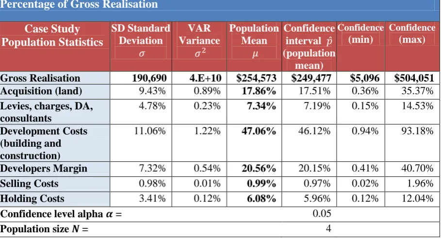
Variability in the case studies can be appreciated with reference to Table 1, where the extent of the variability between case studies is explored with reference to the SD Standard Deviation , VAR Variance , and Population Mean for all major cost components. The confidence interval ̂ (for the population mean) with a confidence level alpha of 0.05 is completed for each of the major cost components and relative percentage proportions of (1) Acquisition (land) cost, (2) Levies, charges, DA, consultants; (3) Development Costs (building and construction); (4) Developers Margin; (5) Selling Costs; and (6) Holding Costs. Since the population size is only 4 (i.e., four case studies), financially “significant” differences may not be statistically significant, but confidence intervals nevertheless do highlight the significant variability between the case studies, and provide a comparison between the extent of the variables with respect of each individual cost component. For example, the confidence interval ̂ for selling costs @ 0.97% and standard deviation of 0.98% is at the extreme low end of variability, compared to development costs (building and construction) which, at a confidence interval ̂ of 47.06% and standard deviation of 11.06%, are at the extreme high end of variability.
Table 1 - Case Study population statistics: variations in cost components as a percentage of gross realisation
Percentage of Gross Realisation
Case Study Population Statistics
SD Standard Deviation
VAR Variance
Population Mean
Confidence interval ̂ (population
mean)
Confidence
(min)
Confidence
(max)
Gross Realisation 190,690 4.E+10 $254,573 $249,477 $5,096 $504,051
Acquisition (land) 9.43% 0.89% 17.86% 17.51% 0.36% 35.37%
Levies, charges, DA, consultants
4.78% 0.23% 7.34% 7.19% 0.15% 14.53%
Development Costs (building and construction)
11.06% 1.22% 47.06% 46.12% 0.94% 93.18%
Developers Margin 7.32% 0.54% 20.56% 20.15% 0.41% 40.70%
Selling Costs 0.98% 0.01% 0.99% 0.97% 0.02% 1.96%
Holding Costs 3.41% 0.12% 6.08% 5.96% 0.12% 12.04%
Confidence level alpha = 0.05
Verification of the theoretical modelling
In authenticating the theoretical model, best fit trend equations – linear or non-linear - can be established for each case study based on the dependant variable (once again, measured by the mortgage repayment equivalent as derived from the quantum of holding costs, expressed as a % of mean household income,) and the independent variable , this time being the length of development period. Thus we can establish a “Holding Cost - Housing
Affordability Trend Line” based on actual results for each specific (i.e. case study) property development. A significant point here is that the “Holding Cost - Housing Affordability
Trend Line” has the ability to determine the impact of shortened or lengthened time frames on housing affordability – whatever their cause.
To explain further, the “Holding Cost – Housing Affordability Trend Lines” plot the equation depicting the length of development period against the cost of mortgage payment equivalent due to holding costs as a percentage of mean household income. These trend lines therefore establish the impact of holding costs over time against housing affordability, both for the theoretical model and actual cases. This provides an indication of the theoretical impact for either shortened or lengthened time-frames, as well as the “actual” result.
However, since the relationship is not always straight line, it may be necessary to choose an alternative functional form of the two variable linear regression model shown at Equation 1 which assumes that, with being the constant, the dependant variable is a linear function of an independent variable under the general formula (Pindyck & Rubinfeld, 1987, p. 47; Studenmund, 2010, p. 15 and others):
Equation 1 Linear (two variable regression) form
i OR alternatively
say the regression coefficient R2 alone); however selection is optimally based on the model exhibiting logically non-linearity characteristics, even though the exact form of the nonlinearity may not be readily apparent. As stated by Studenmund (2010, p. 229), “a choice
between the non linear forms cannot be made on the basis of economic theory”. Pindyck & Rubinfeld (1987, pp. 108-109) suggest that choosing regression parameters is equivalent to finding the best parabola which fits the point on a two dimensional graph of and . The resultant quadratic form is therefore useful for testing nonlinearities. These alternate forms considered (tested for goodness of fit) could include:
Equation 2 Polynomial form
i ( i) i i
Equation 3 Exponential form
( )
Equation 4 Logarithmic (semilog) form
Where = the dependant variable (i.e. Holding Costs)
‘s = independent or explanatory variables (e.g. in this case, interest rates, inflation, and time frames for statutory approvals and overall holding period(s), etc).
= stochastic error term
= constant or intercept of the equation (denoted in the single equation model)
= ith observation
= natural log
Testing under the multiple linear form, where appropriate, is conducted under the formula at Equation 5:
Equation 5 Multiple linear regression analysis form
i i i i
‘s are non-stochastic, with no exact linear relationship existing between two or more of the independent variables (i.e. no perfect multicollinearity)
Error term has 0 expected value (mean) and constant variance for all observations (i.e. no heteroskedasticity)
Errors corresponding to different variations are uncorrelated
Error variable is normally distributed
It is pointed out that the usefulness of testing under the multiple linear form is limited. For example, multicollinearity issues when using multiple regression models (i.e. problems between some variables where there is already a clear existing relationship - one obvious example in this instance might be inflation rate, and interest rate, but such problems are largely dependent upon the particular time period selected)1.
There may also be limitations due to sample size, i.e. as a general rule it is accepted that as the number of observations increase, the reliability of the obtained correlations also increases; on the other hand, if the sample size is sufficiently large virtually any null hypothesis can be rejected – often found to be a problem in finance2. However, even though sample size is problematic in this example (the case studies relate to large residential developments where there are typically very limited transactions occurring), the regression analysis conducted nevertheless informs by: (1) determining indicative sensitivity (slope of the regression trend) of the base case scenario independent variables, which is also confirmed and tested by the case study data; and (2) developing a table of cross sectional bivariates to assist in interpretation of the Holding Cost – Housing Affordability trend lines.
This leads to consideration of the institutional context, and the inability often experienced by researchers concerning non-disclosure of transactional details (a point not lost on AHURI researchers recently)3, and limited market evidence. Notwithstanding the foregoing, in this instance, it is more important to ensure a focus on the quality of responses,
1 This is overcome by using certain methods such as transforming the highly correlated variable into a ratio and
using that as the ; ignoring it (if the model is otherwise adequate in terms of each coefficient being of a plausible magnitude); collation of additional data and / or changing the time period where possible; or even eliminating one of the collinear variables if deemed necessary.
2 In real estate where, as in this case, sample sizes are often very small, a 5 per cent significance level is widely
used (Brooks & Tsolacos, 2010, pp. 62-63). Other “ rules of thumb” indicate that the sample size should be not less than 10 times the number of variables (Comrey & Lee, 1992), or utilising at least 30 observations to estimate even the simplest models, and at least 100 is desirable (Brooks & Tsolacos, 2010, p. 66). Traditionally, statisticians prefer larger sample sizes of 200 (Comrey & Lee, 1992, p. 200 - sample sizes of 200 rates as "fair", and 300+ rates as "good"), i.e. the more complex models rely heavily on available information and therefore require larger quantities of data. It is recognised that sampling error is minimised by increasing the size of the sample since small samples are more likely to be inherently unrepresentative. Other problems with obtaining a small sample size relate to the nature of real estate data, in particular the infrequency of transactions, and evidence of yields, rents (if applicable) and prices.
3 It was recorded by researchers that their overall analysis of planning costs was limited by a lack of financial
data provided by the sample of case study developers. In itself, this inability or unwillingness to provide specific cost data on planning related expenses supports claims that this information is difficult to ascertain with
rather than relying upon response numbers. In this regard, the most important criteria in relation to sampling is to obtain a survey from participants in a highly specific target property development market.
Use of a cross sectional model
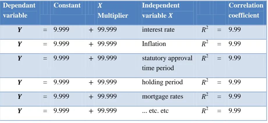
Development of a cross sectional regression model, of the kind used to explain yield differences between global real estate markets (Hollies, 2007) may appropriate to assist interpretation. Output consists of a series of bivariate regressions estimated to assess the explanatory ability of determinate variables on the dependant variable. For instance, in this example a model can be developed along the lines generically expressed at Table 2.
Table 2 Concept of the cross sectional regression table Dependant
variable
Constant
Multiplier
Independent variable
Correlation coefficient
= 9.999 99.999 interest rate = 9.99
= 9.999 99.999 Inflation = 9.99
= 9.999 99.999 statutory approval time period
= 9.99
= 9.999 99.999 holding period = 9.99
= 9.999 99.999 mortgage rates = 9.99
= 9.999 99.999 ... etc. etc = 9.99
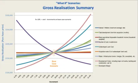
A summary of data modelling for each of nine independent variables, along with their best fit regression equations (i.e. impact on holding costs) is shown at Figure 2. The housing affordability curves provide a comparative overview of all variables (Figure 4).
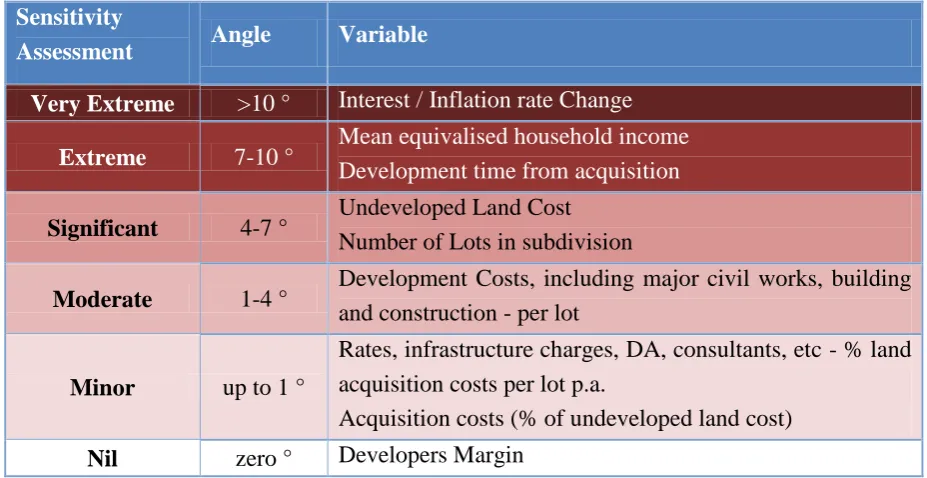
The table of bivariate regressions enables the sensitivity of the independent variables to be demonstrated both statistically, and visually, as per Appendix 1: Linear Trend line Analysis - Sensitivity of Factors Impacting Holding Costs and Subsequent Effect on Housing Affordability. The output of that analysis is summarised at Table 3; it contains critical results from which we can derive our conclusions. For example, this analysis shows that interest rates and development timeframes are critical to the holding cost equation. Whilst this result broadly confirms the general thrust of the literature on the topic, it also highlights that the extent of these impacts may not have been hitherto fully appreciated.
correspondingly limited impact on housing affordability. This is important in the context of housing affordability, since a factor could have a limited or even no impact on holding costs, yet have a significant impact on housing affordability because it affects gross realisation prices. A good example of this is the developer’s margin: it has no impact on holding costs at all, yet could be significant for end-users. In this regard, comparisons can be made between Figure 2 and Figure 3 for different variables.
Table 3 Sensitivity of factors impacting holding costs, and subsequent effect on housing affordability
Sensitivity
Assessment Angle Variable
Very Extreme >10 ° Interest / Inflation rate Change
Extreme 7-10 ° Mean equivalised household income Development time from acquisition
Significant 4-7 ° Undeveloped Land Cost
Number of Lots in subdivision
Moderate 1-4 ° Development Costs, including major civil works, building
and construction - per lot
Minor up to 1 °
Rates, infrastructure charges, DA, consultants, etc - % land acquisition costs per lot p.a.
Acquisition costs (% of undeveloped land cost)
Figure 2 “What-If” Scenarios: Holding Costs summary of all independent variables
Figure 3 “What-If” Scenarios: Gross Realisation summary of all independent variables
$0 $5,000 $10,000 $15,000 $20,000 $25,000 $30,000 $35,000 $40,000 $45,000 H o ld in g C o st s Increment
Interest / Inflation (maximum average) rate:
Total development time from acquistion (months)
Mean equivalised disposable household income (household weighted)
Number of Lots in subdivision:
Undeveloped Land Cost
Acquistion costs (% of undeveloped land cost)
Rates / infrastructure levies / charges, DA, consultants, etc.
Development Costs, including major civil works, building and construction - per lot
Developers Margin
9 x 10% + and - increments on base case scenario
Base Case Scenario $100,000 $150,000 $200,000 $250,000 $300,000 G ro ss R e al is at io n ( P u rc h as e p ri ce ) Increment
Interest / Inflation (maximum average) rate:
Total development time from acquistion (months)
Mean equivalised disposable household income (household weighted)
Number of Lots in subdivision:
Undeveloped Land Cost
Acquistion costs (% of undeveloped land cost)
Rates / infrastructure levies / charges, DA, consultants, etc.
Development Costs, including major civil works, building and construction - per lot
Developers Margin
9 x 10% + and - increments on base case scenario
Holding cost – housing affordability trend lines
The final part of the econometric modelling in this example establishes “best fit” trend equations – linear or non-linear - for each of the case studies, based on the dependant variable (once again, measured by the mortgage repayment equivalent as derived from the quantum of holding costs, expressed as a % of mean household income,) and the independent variable
, being the length of development period.
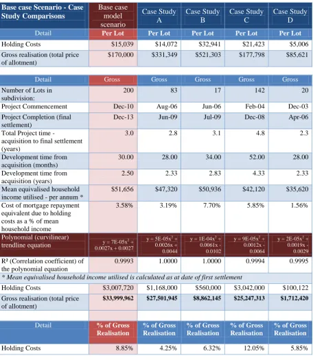
First, we establish the “Holding Cost - Housing Affordability Trend Line” (which is shown at Figure 4). This is achieved by inputting the actual results for each specific property development project (along with a base case scenario) into a Holding Cost model. The baseline data inputs, and the primary outputs of the model is shown at Appendix 2: Case Study Comparisons against the Base case Scenario (summary data).
It is then possible to run the best fit linear or non-linear trend analysis on the “Holding
Cost - Housing Affordability Trend Lines”, which in this case results in polynomial regression equations which are summarised at Table 4. Here, polynomial regression equations are used to solve for the housing affordability variable .
Figure 4 Holding Cost – Housing Affordability Trend Lines
3.58%
3.19%
7.70%
5.85%
1.56% 0%
5% 10% 15% 20% 25% 30%
1.0 1.5 2.0 2.5 3.0 3.5 4.0 4.5 5.0 5.5 6.0
Affordability (mortgage equivalent) % is labelled on trendline
Table 4 Polynomial trend line equations summary for case studies and the Holding Cost Economic Model base case scenario
Base case Scenario - Case Study Comparisons Base case model scenario Case Study A Case Study B Case Study C Case Study D
Detail Per Lot Per Lot Per Lot Per Lot Per Lot
Holding Costs $15,039 $14,072 $32,941 $21,423 $5,006
Gross realisation (total price of allotment)
$170,000 $331,349 $521,303 $177,798 $85,621
Detail Gross Gross Gross Gross Gross
Number of Lots in subdivision:
200 83 17 142 20
Project Commencement Dec-10 Aug-06 Jun-06 Feb-04 Dec-03
Project Completion (final settlement)
Dec-13 Jun-09 Jul-09 Dec-08 Apr-06
Total Project time -
acquisition to final settlement (years)
3.0 2.8 3.1 4.8 2.3
Development time from acquisition (months)
30.00 28.00 34.00 52.00 28.00
Development time from acquisition (years)
2.50 2.33 2.83 4.33 2.33
Mean equivalised household income utilised - per annum *
$51,656 $47,320 $50,936 $42,120 $35,620
Cost of mortgage repayment equivalent due to holding costs as a % of mean household income
3.58% 3.19% 7.70% 5.85% 1.56%
Polynomial (curvilinear)
trendline equation y = 7E-05x
2 +
0.0027x + 0.0027
y = 5E-05x2 +
0.0026x + 0.0044
y = 1E-04x2 +
0.0061x - 0.0102
y = 9E-05x2 +
0.0012x - 0.0064
y = 2E-05x2 +
0.0019x - 0.0029
R² (Correlation coefficient) of the polynomial equation
0.9993 1.0000 1.0000 0.9994 0.9995
* Mean equivalised household income utilised is calculated as at date of first settlement
Holding Costs $3,007,720 $1,168,000 $560,000 $3,042,000 $100,122
Gross realisation (total price of allotment)
$33,999,962 $27,501,945 $8,862,145 $25,247,313 $1,712,420
Detail % of Gross Realisation
% of Gross Realisation
% of Gross Realisation
% of Gross Realisation
% of Gross Realisation
Appendix 1 - Linear Trend line Analysis: Sensitivity of Factors Impacting Holding Costs and Subsequent Effect on Housing Affordability
Sensitivity* Very
Extreme
Extreme Significant Moderate Minor Nil
>10 deg 7-10 deg 4-7 deg 1-4 deg up to 1 deg zero deg
"What If" Scenario: Interest / Inflation rate Change Mean equivalised household income Development time from acquisition Undeveloped Land Cost Number of Lots in subdivision Development Costs- per lot
Rates, infrastructure charges, DA, consultants, etc - Acquisition costs (% of undeveloped land cost) Developers Margin Regression Formula # y=0.0078x - 0.00241 y= 0.0041x +0.0833
y = 0038x - 0.0046
y = 0.0027x + 0.012
y = 0.0029x + 0.699
y = 0.0011x + 0.0264
y = 0.0004x + 0.0326
y = 8E-05x + 0.0351
y = 3E-18x + 0.0358 R2 # 0.8452 0.9336 0.9002 0.9554 0.9336 0.9554 0.9554 0.9564 0.00E+00 Regression
Formula (forced intercept@ zero)
y = 0.0059x n/a y = 0.0042x y = 0.0036x n/a y = 0.0031x y = 0.0029x y = 0.0028x y = 0.0028x
R2 (forced
intercept zero) 0.7826 n/a 0.8904 0.813 n/a 3.496 -54.4 -1444 3.00E+14 x Coefficient
(forced)] 0.0059 0.0041 0.0042 0.0036 0.0029 0.0031 0.0029 0.0028 0.0028 Arctangent, in
degrees (forced) 0.34 0.23 0.24 0.21 0.17 0.18 0.17 0.16 0.16
Width 4.33 2.33 2.14 1.69 1.55 0.38 0.27 0.07 0.00
Height 14.05 15.85 15.75 15.90 15.84 15.91 15.91 15.89 16.76
Tangent of the
linear trend 0.31 0.15 0.14 0.11 0.10 0.02 0.02 0.00 0.00
Angle4 17.13 -8.36 7.74 6.07 -5.59 1.37 0.97 0.25 0.00
Linear Trend Analysis - conducted on cost of mortgage repayment as a result of holding costs as a % of equivalised disposable household income
* Sensitivity - based on angle of variable (arctangent [inverse tangent], in degrees) achieved in + - 10% incremental shifts # Unforced intercept
Appendix 2: Case Study Comparisons against the Base case Scenario (summary data)
Base case Scenario - Case Study Comparisons: Summary Data
Base case model scenario
Case Study A Case Study B Case Study C Case Study D
Detail Per Lot Per Lot Per Lot Per Lot Per Lot
Acquisition cost (undeveloped land) $38,663 $49,771 $107,941 $50,627 $5,225
Rates, infrastructure levies / charges, DA, consultants,
special council charges & land tax $7,733 $26,687 $34,529 $23,585 $1,400
Development Costs, including major civil works, building
and construction $75,000 $167,048 $227,824 $68,887 $55,000
Developers Margin $27,287 $72,122 $112,906 $11,516 $16,658
Selling Costs $6,279 $1,649 $5,161 $1,760 $2,332
Holding Costs $15,039 $14,072 $32,941 $21,423 $5,006
Gross realisation (total price of allotment) $170,000 $331,349 $521,303 $177,798 $85,621
Number of Lots in subdivision: 200 83 17 142 20
Project Commencement Dec-10 Aug-06 Jun-06 Feb-04 Dec-03
Project Completion (final settlement) Dec-13 Jun-09 Jul-09 Dec-08 Apr-06
Total Project time - acquisition to final settlement (years) 3.0 2.8 3.1 4.8 2.3
Development time from acquisition (months) 30.00 28.00 34.00 52.00 28.00
Development time from acquisition (years) 2.50 2.33 2.83 4.33 2.33
Developers Margin 20.0% 28.0% 28.0% 7.0% 25.0%
Mean equivalised household income utilised - per annum * $51,656 $47,320 $50,936 $42,120 $35,620 Cost of mortgage repayment equivalent due to holding
costs as a % of mean household income 3.58% 3.19% 7.70% 5.85% 1.56%
Polynomial (curvilinear) trend line equation y = 7E-05x2 + 0.0027x + 0.0027
y = 5E-05x2 + 0.0026x + 0.0044
y = 1E-04x2 + 0.0061x - 0.0102
y = 9E-05x2 + 0.0012x - 0.0064
y = 2E-05x2 + 0.0019x - 0.0029
R² (Correlation coefficient) of the polynomial equation 0.9993 1.0000 1.0000 0.9994 0.9995
References
Barnett, W., Hendry, D. F., Hylleberg, S., Teräsvirta, T., Tjøstheim, D., & Württz, A. (Eds.). (2000). Nonlinear Econometric Modelling in Time Series Analysis: Proceedings of the Elevennth International Symposium in Economic Theory and Econometrics. New York: Cambridge University Press.
Brooks, C., & Tsolacos, S. (2010). Real Estate Modelling and Forecasting: Cambridge.
Comrey, A. L., & Lee, H. B. (1992). A first course in factor analysis (2nd ed.): Hillsdale, Lawrence Erlbaum Associates.
Garner, G. O. (2012). An Analysis of Holding Cost Impact on Housing Affordability in Relation to Midsized Greenfield Residential Property Developments in South East Queensland. Doctor of Philosophy, Queensland University of Technology, Australia, Brisbane. (Final Version)
Gurran, N., Ruming, K., & Randolph, B. (2009). Counting the costs: planning requirements, infrastructure contributions, and residential development in Australia: Australian Housing and Urban Research Institute.
Hollies, T. (2007). International variation in office yields: a panel approach. Journal of Property Investment & Finance, 25(4), 370-387.
Pindyck, R. S., & Rubinfeld. (1987). Econometric Models and Economic Forecasts (2nd ed.): McGraw-Hill International.