DEVELOPMENT OF CALIBRATION
SCHEME AND SOFTWARE FOR
DOPPLER LIDAR RECEIVER
K RAGHUNATH*
National Atmospheric Research Laboratory, Department of Space, Gadanki- 517 112, India e mail: [email protected], Tel: +91-8585-272014, Fax: +91-8585-272018
(corresponding author)
DV ABHINAVA KARTHIK
Sophomore, Department of Electronics and Communications Engineering, JNT University, Hyderabad- 500 085, India,
e mail: [email protected]
S NARAYANA REDDY
Department of Electrical and Electronics Engineering, SV University, Tirupati- 517 502, India e mail: [email protected]
K RAMESH
Sophomore, Department of Physics, SV University, Tirupati- 517 502, India e mail: [email protected]
Abstract
An Incoherent Doppler lidar (laser radar) is being developed at National Atmospheric Research Laboratory, Gadanki(13.5ºN, 79.2ºE), India to measure winds in troposphere and stratosphere. The lidar has a stabilised laser source, a telescope and a receiver. In the receive chain, the system employs a servo stabilised Fabry-Pérot Interferometer as a narrow pasband filter for measuring wind velocities. Calibration of receive chain with Fabry-Perot Interferometer is crucial for deriving the wind velocities. The developed calibration scheme gives two informations, one, the exact operation point of the Fabry-PérotInterferometer and the second to generate “Look-up table” which is useful in deducing the winds. A software is developed for the purpose which is tested independently.
Keywords: Lidar; calibration; algorithm.
1. Introduction
2. Lidar system
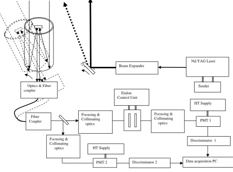
The lidar system is a monostatic biaxial system with the laser output derived from a frequency doubled Nd:YAG laser. The expanded laser beam is of 80 mm size and the output power is 30W with Pulse Repetition rate of 50pps. The laser is injection seeded with a stable, narrow line width CW fiber laser. The receiver is 350mm Cassegrain feed telescope with F number of 11 which is fiber coupled to rest of the optics. The optical fiber has a Numerical Aperture of 0.37 with core diameter of 1.5mm. The fiber diameter decides the Field of view of the receiver. In NARL Doppler lidar system single edge technique is adopted for its effectiveness. The specifications are given in Table 1.
The output of the fiber is divided into two parts in 1:9 ratio. Greater part goes to the channel containing FPI functioning as frequency discriminator and smaller part goes to the Energy monitor channel. The FPI channel senses the change in the signal transmission as the Doppler shift and second channel without FPI senses the energy changes, if any. The ratio between signals from two channels gives normalised signal. The two channels, from then have identical components. Radial velocities are calculated from Doppler spectral shifts. The horizontal wind components are obtained with Doppler Beam swinging technique. The generic block diagram is shown in Fig 1. The PMT, used as a photodetector, sends negative going pulses to a fast discriminator for removing noise component. After pulse shaping the signal is given to a Multichannel scalar card for photon counting.
Multi-Channel Scaler (MCS) operates with a Windows based software‚ and all controls and spectral manipulations are implemented via on-screen displays. A dual-port memory on the card displays spectral data, without interrupting data acquisition by the MCS. When a scan is started, the MCS begins counting the input event in the first channel of its digital memory. At the end of the preselected dwell time, the MCS advances to the next channel of memory to count the event. This dwell and advance process is repeated until the MCS has scanned through all the channels in its memory. In our case, the photon strength is presented with respect to lapse time and is initiated with a trigger pulse synchronising with observations.
Figure 1: A generic Block diagram of an Incoherent Doppler lidar system Beam Expander
Nd:YAG Laser
Seeder Optics & Fiber
coupler
HT Supply
PMT 1 Focusing &
Collimating optics
Focusing & Collimating optics Etalon
Control Unit
Focusing & Collimating optics
Discriminator 2 PMT 2
HT Supply
Data acquisition PC Discriminator 1
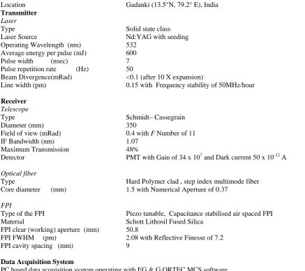
Table 1: Specifications of the lidar system
______________________________________________________________________________
Location Gadanki (13.5°N, 79.2° E), India
Transmitter
Laser
Type Solid state class
Laser Source Nd:YAG with seeding
Operating Wavelength (nm) 532 Average energy per pulse (mJ) 600
Pulse width (nsec) 7
Pulse repetition rate (Hz) 50
Beam Divergence(mRad) <0.1 (after 10 X expansion)
Line width (pm) 0.15 with Frequency stability of 50MHz/hour
Receiver
Telescope
Type Schmidt– Cassegrain
Diameter (mm) 350
Field of view (mRad) 0.4 with F Number of 11 IF Bandwidth (nm) 1.07
Maximum Transmission 48%
Detector PMT with Gain of 34 x 107 and Dark current 50 x 10-12 A
Optical fiber
Type Hard Polymer clad , step index multimode fiber
Core diameter (mm) 1.5 with Numerical Aperture of 0.37
FPI
Type of the FPI Piezo tunable, Capacitance stabilised air spaced FPI Material Schott Lithosil Fused Silica
FPI clear (working) aperture (mm) 50.8
FPI FWHM (pm) 2.08 with Reflective Finesse of 7.2 FPI cavity spacing (mm) 9
Data Acquisition System
PC based data acquisition system operating with EG & G ORTEC MCS software
Bin width (Range Resolution) (μsec) 2 corresponding to 300m with Time Integration of 250 sec
The laser and FPI play a key role in wind observations and hence it is important to monitor its characteristics. A wavelength meter, model WS U-10 of High Finesse with absolute accuracy of +/- 10MHz, is used to measure line width and wavelength stability of the seeded laser. The laser characteristics have been monitored for several hours. The line width is consistently giving about 0.3 pm with wavelength drifts of about ~ 0.015pm which corresponds to ~300MHz and ~15MHz/hr respectively in frequency @532nm.
The specifications of the servo-stabilized Fabry-Pérot Interferometer is given in Table 1. The system comprises FPI and control unit. The control unit is a three-channel (X Y Z) controller, which uses capacitance micrometers and PZT actuators to monitor and correct errors in mirror parallelism and spacing. The FPI is mounted on an XYZ mount for adjusting the input angle of incidence from optical fiber and thus additional control on the FPI. The Airy distribution of the FPI obtained by scanning the FPI spacing with a stabilised HeNe laser gives a Finesse of ~8.0 @632.99nm. Both these measurements viz, laser and FPI are suitable for carrying out atmospheric mean wind measurements.
Data analysis /wind derivation
The shift in the frequency due to wind is computed from the well known edge technique formulations [Korb et al (1992)]
fD = ∆I N /β (1)
∆I N is Doppler shift given by
∆I N = [F(ν+∆ν) - F(ν)] Where
F(ν) = IN (ν) is the normalised reference signal i.e zenith beam in this case
F(ν +∆ν) = IN (ν+∆ν) is the normalised oblique signal which contains radial velocity information
β is the average slope of the edge filter function as observed with reference signal From the frequency shifts, wind velocity is determined.
3. Calibration method
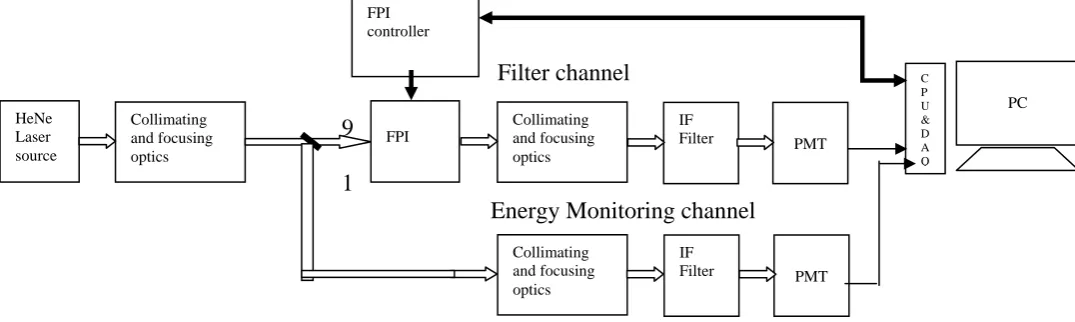
The lidar needs to be calibrated for proper wind derivation. In Single Edge technique, operation of FPI at its most sensitive point is important which is usually at the slope of the characteristics of the FPI. The functional block diagram to know these coordinates is shown in Fig 3. The flow chart for executing the scheme is shown in Fig 4.
The software is developed using Visual C++ language, using FPI software commands, MCS data acquisition software commands. The code running to about 1200 lines does two tasks simultaneously.
a) Access the FPI Control unit and scan the z (etalon spacing) value between starting and ending Points:
After initializing the FPI control unit, all the given input values are sent to the FPI controller from the PC. Scanning between starting and ending points is enabled by the User by giving values. On START, z value is incremented, the incremental values of which are calculated as per given number of sampling points.
Increment = (ending point – starting point) / No of sampling points. New z value = current z value + increment.
Current z value is periodically executed and sent to the controller. MCS job also starts immediately after pressing START scan button. The detected signal from PMT is recorded by MCS card. The initiation of data acquisition and scanning are executed in sync which leads to creation of distinct MCS profile for each z value. This procedure repeats until z value reaches the End point. On reaching end value, z is decremented by same magnitude and sent to the controller. This process repeats continuously until STOP is activated.
Filter
channel
9
1
Energy Monitoring channel
Figure 3: Calibration scheme for the lidar receiver
b) Read the data from MCS profile for calculating channel ratio and slope:
After executing each z value, corresponding MCS profile is generated as described above. To display the ratio between FPI/filter channel and energy-monitoring channel, each MCS profile is read after completing. The Calibration Software keeps checking for the creation of MCS profile and if so, the file is read for further processing. To account for any laser energy instabilities, the average of all the signal collected in one profile i.e for one z value is taken. Ratio and Slope can be calculated from two MCS channels i.e “FPI channel” and “energy monitoring channel” using the relations,
Ratio between two channels = Filtered channel signal avg value / Energy monitoring channel signal avg value Slope is given by dT/ dz, where dT= difference between present and previous transmission values of ratio
and dz=z spacing between two scans ( Z increment or decrement value )
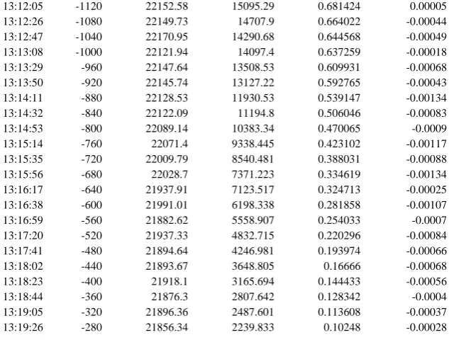
Measured signal intensities in FPI channel and energy monitoring channel and calculated slope and ratios and are plotted with respect to z value for display and the ASCII data is saved in given file name. The sample data saved is shown in Table 2. The display screen for the software is shown in Fig 5.
HeNe Laser source Collimating and focusing optics Collimating and focusing optics FPI IF
Filter PMT
Collimating and focusing optics
IF
NO
YES
NO
YES
Figure 4: RDL Receiver calibration software flowchart
START
Initialize the CS100 controller & read the MCS Job file.
IF start Pressed
Read the input parameters and send to the controller
Increase the Z value from starting point as per number of sampling points and send Z value to the controller,
Start MCS job as per given Job file
Wait for MCS profile to complete and read data from that file, Calculate the ratio, dT/ dz
Display the ratio and dT/dz and save the output data in given file
IF Stop Pressed
Figure 5: The Rayleigh Doppler lidar Receiver calibration software (a) Depicts signal in “Energy Monitoring channel (b) in FPI “channel” (c) Calculated “Ratio of the two channels” (d) Calculated change in transmission with FPI spacing i.e dT/dZ . The second profile running over the first one in all the panels is generated when FPI is scanned in the opposite direction
Time
z value
without FPI
with FPI
Ratio dT/dz
13:12:05 -1120 22152.58 15095.29 0.681424 0.00005 13:12:26 -1080 22149.73 14707.9 0.664022 -0.00044 13:12:47 -1040 22170.95 14290.68 0.644568 -0.00049 13:13:08 -1000 22121.94 14097.4 0.637259 -0.00018 13:13:29 -960 22147.64 13508.53 0.609931 -0.00068 13:13:50 -920 22145.74 13127.22 0.592765 -0.00043 13:14:11 -880 22128.53 11930.53 0.539147 -0.00134 13:14:32 -840 22122.09 11194.8 0.506046 -0.00083 13:14:53 -800 22089.14 10383.34 0.470065 -0.0009 13:15:14 -760 22071.4 9338.445 0.423102 -0.00117 13:15:35 -720 22009.79 8540.481 0.388031 -0.00088 13:15:56 -680 22028.7 7371.223 0.334619 -0.00134 13:16:17 -640 21937.91 7123.517 0.324713 -0.00025 13:16:38 -600 21991.01 6198.338 0.281858 -0.00107 13:16:59 -560 21882.62 5558.907 0.254033 -0.0007 13:17:20 -520 21937.33 4832.715 0.220296 -0.00084 13:17:41 -480 21894.64 4246.981 0.193974 -0.00066 13:18:02 -440 21893.67 3648.805 0.16666 -0.00068 13:18:23 -400 21918.1 3165.694 0.144433 -0.00056 13:18:44 -360 21876.3 2807.642 0.128342 -0.0004 13:19:05 -320 21896.36 2487.601 0.113608 -0.00037 13:19:26 -280 21856.34 2239.833 0.10248 -0.00028
Table 2: Output of the software showing generated values for scantime of about 15 minutes.
Once the receiver calibration data is known, the operating point i.e z spacing is chosen where the FPI profile is sharp. In this case the operating point is -600. The ratio dT/dz for different FPI spacings is considered in the Eq 1 for deriving Doppler frequency shifts.
4. Conclusions
A calibration scheme and software is developed for NARL Doppler lidar system. This is tested and is working as envisaged. The resultant values are useful in identifying the operating point for actual observations and in calculating Doppler frequency shifts.
References
[1] Gentry Bruce M , Huailin Chen, Steven X Li (2000): Wind measurements with 355-nm molecular Doppler lidar , Optics. Letters., Vol. 25, No.17
[2] Korb C Laurence , Bruce M Gentry Chi Y Weng (1992): Edge technique: theory and application to the lidar measurement of atmospheric wind, Applied Optics., 31
[3] Korb L , BM Gentry, SX Li, C Flesia (1998): Theory of double-edge technique for Doppler lidar wind measurements, Applied. Optics., Vol37, No 15
[4] LIU Zhishen , et al (2003): A mobile incoherent Mie-Rayleigh Doppler wind lidar with a single frequency and tunable operation of an injection Nd:YAG laser, Science in China (Series E), 46, 309-316
[5] Souprayen C, et al (1999): Rayleigh-Mie Doppler wind lidar for atmospheric measurements. I Instrumental setup, validation and first climatological results, Applied Optics., Vol 38, No.12
[6] Tepley C A, Stoyan I Sargoytchev, Roberto Rojas (1993): The Doppler Rayleigh Lidar System at Arecibo, IEEE Trans. on Geoscience and Remote Sensing, Vol. 31, No.1
[7] von Zahn U , et al (2000): The ALOMAR Rayleigh/Mie/Raman lidar: objectives, configuration, and performance, Ann. Geophysicae 18
[8] Xia Haiyun, et al (2007): Fabry–Pérot interferometer based Mie Doppler lidar for low tropospheric wind observation, Applied Optics.,46, 7120-7131