Contrasting Availability-Aware Energy-Optimized VM Scheduling Algorithms

1711

Contrasting Availability-Aware Energy-Optimized

VM Scheduling Algorithms

Abstract— Data Centers have been rapidly increasing in number and size and are poised for even more significant growth in the future. These Data Centers consume significant energy leading to increased cost and damage to the environment, leading to the conservation of energy in Data Centers being one the increasingly important areas of focus. There have been several approaches and algorithms devised for optimizing the energy consumed by Data Center active components viz. compute, storage, and networking. These algorithms or approaches typically focus solely on Energy Efficiencies whereas Applications would also have QoS expectations like Availability which may have a trade-off. This paper explores two of the Biologically inspired VM scheduling algorithms, the Genetic and the Particle Swarm Optimization Algorithms that incorporate Energy Efficiencies along with considerations towards Availability. We also evolve a mechanism that will map the QoS Availability percentage expectation of a VM to a replication factor, which can help determine the number of replicas that are needed to support the expected Availability. The resulting energy consumption in Data Centers is contrasted against a baseline are published algorithms to demonstrate efficiencies achieved with Availability constraints.

Index Terms—Cloud Data Centers, Energy optimization, Availability, Failure rate, Genetic Algorithm, Particle Swarm Optimization PSO, Gravity Algorithm

——————————  ——————————

1

I

THE rising popularity and growth of data-hungry applications and services are driving the growth of Data Centers in scale and power consumption. It is estimated that there would be 50 billion connected devices by 2020, creating large amounts of data to be stored and processed in huge Data Centers. At this rate of growth, Data Centers are expected to consume almost 20% of all the electricity generated in the world, which in turn would lead to ~5.5% of the global carbon footprint created along with 2% of the total greenhouse gas emissions. Several approaches have been explored around the active components like Compute, Storage, Network of the Data Center to reduce energy consumption. Compute elements in the granularity of VMs, which is one of the significant contributors to this energy consumption, is the focus of our work. Scheduling VMs into a physical host involves considering the resource requirements and applying the designed constraints towards energy, Availability and then associating a Physical Server to it. Significant number of the approaches which support the energy constraints for VMs, look to increase the utilization of Servers by consolidating the application instances into a minimum number of Servers (thus lowering number of Servers needed and hence the energy), which could lead to a single point or zone of failure, leading to an impact on the Availability. These approaches do not directly factor in the Availability requirements of the VMs which may need some trade-offs. In this paper, we look at a few of the VM Scheduling approaches which focus only on energy efficiencies and those which consider Availability and energy, leading to the motivation and our goal outcomes. We then discuss our Availability Model, the Algorithms under our consideration and the Adaptations to them. We then discuss the simulation framework used, the configurations, workloads used, the simulations were done and results and our observations from the results.

2 R

W

VM Scheduling approaches orchestrate the Physical Servers to provision for the requirements as requested by the Applications within the Data Center infrastructure. This would begin by factoring in the availability of unused capacity for the resource size requested and then applying the constraints like performance & energy reduction. Approaches with energy optimization objective, look to reduce the total number of Physical Servers needed to be in an Active power-consuming state, by using efficient algorithms for placement and/or consolidation through migration. There have also been approaches explored that move the Physical Servers into low power consumption Operating modes. Since cooling contributes significantly to the total energy consumed in the Data Center, there are approaches for VM Scheduling which factor in the cooled state of the Data Center components e.g. Phalachandra et al [18] consider fine-grain Data Center Component cooling and schedule VMs into already cooled components, and optimize the need for cooling with encouraging results. Approaches as with DENS[8], VM Consolidation Algorithms by Buyya et.al [9][10], Khan et.al [11], Elastic Tree [12], Green Cloud [13], VMPlanner [14] look at approaches for consolidating the VM requirements into fewer Physical Servers, facilitate moving the idle servers after allocation, into low power consumption states as part of allocation. There have also been approaches that have looked to manipulate the VM allocation based on Utilization [21] and Dynamically placing VMs into Physical Machines [22]. Some approaches look at modeling the cost of Migration for energy and performance and then support the VM migration based on it [23]. There are temperature aware VM Scheduling algorithms like with the Zone-Based Discretization (ZBD), where power allocation to Servers in Active power-consuming area is managed to prevent localized heat buildup, and look to reduce energy consumption by Minimizing Heat recirculation (MinHR) as in [16]. The work by Cao et al [17] looks to reduce hotspot temperatures by optimizing/reducing placement of high energy consumption jobs into homogeneous high-performance computing (HPC) clusters, by placing it on systems that least contribute to Hot spots. All of these proposed approaches predominantly look for exact solutions for energy based on a linear program described by a small number of inequalities. These do not support finding solutions optimally within a reasonable time and problems involving the allocation of a large number of items (or VMs) to many bins (or

————————————————

 Phalachandra HL ([email protected]) and Dr. Dinkar Sitaram ([email protected]) currently drive the Cloud Computing and Big Data Lab in CSE Dept, at PES University, Bangalore, India.

 Rahul M ([email protected]) and Rahul Pillai

1712 Servers). To scale and find solutions for large sizes, heuristics

or metaheuristics-based approaches have also been used to statically/dynamically consolidated the VMs into fewer Servers to reduce the energy consumption of the hosting nodes. There have also been approaches like the ones by Wang et. al [24] and Yang et. al [25] which keep only Availability in context when allocating resources to scale or in the approaches by Jamal et. al [26] where a failover group based on Component failure characteristics is formed for providing Availability. There are fewer approaches that keep Availability as a constraint while optimizing for Energy Efficiencies like the Gravity meta-heuristic by Phalachandra et.al [1], where they allocate VM replicas as needed for the Availability requirement into different granular Failure zones. Scheduling of a VM to a Server within the Failure zone is done using the Gravity Algorithm based on the energy-cost. As part of the Algorithm, the VM to Physical machine association gravitates to a local minimal energy cost from a random candidate starting point, by looking at neighbors for lower energy cost. Iterating similarly for a pre-determined number of times, the algorithm gravitates to a global minimum, to which the VM is scheduled. This approach of Availability factored; energy cost-optimized solution has been found to provide ~17+% efficiency.

3 M

C

Given the promising results seen with the Heuristic-based Gravity algorithm as seen above, our work presented in this paper looks at other Adaptive and Global Optimization Algorithms inspired by population genetics of natural selection the Genetic Algorithm (GA) and Particle Swarm Optimizations (PSO) where selection is based on Swarm Intelligence, where the selections are based on inductive reasoning for solutions, which have also been successfully applied in search and optimization domains with good results. We have adapted both the Genetic Algorithm and Particle Swarm Optimization algorithms to VM scheduling scenario along with the Heuristics based Gravity mechanism which could be used as a baseline for contrast. We have also arrived with a mechanism, where an application can specify the availability needed (as like 99.99%) which is mapped to a certain replication factor. These replicas are scheduled factoring in Failure zones of the environment, and the results thus obtained with availability constraint is contrasted with the non-evolutionary Algorithms being used as baselines. These demonstrate the performance-energy consumption, Availability-performance-energy consumption tradeoff associated with VM Scheduling.

4 A

M

Availability of Compute systems is typically achieved through replication of VMs and in our work we have used the following blocks for modeling Availability.

4.1 Failure Zone

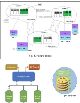
A failure zone is the granular unit of the Data Center which can fail. This failure zone unit could be a VM, a physical server, a rack with a group of servers, a set of racks in a Data Center Aisle, a Sector of Aisles, a zone in the Data Center or the whole Data Center as a unit.

Fig 1. demonstrates the concept of failure zones, where each of the three Data Centers 1,2 and 3 can be considered to be a failure zone. Consider 3 jobs for App1 running on VMs VM1-1, VM2-1, and VM3-1 respectively and App2 running on VM2-1 and App3 running on VM2-1 and VM3-1. The three applications have different Availability needs and hence the number of copies. As shown in the figure, if the Failure zone is designed to be a Data Center, then VM1 with App1 would be hosted into Servers in three different Data Centers as in the figure. If there is only 1 Data Center and the Failure zone is set-up as a Rack, and then the VM with the App will be hosted in three different Racks within the Data Center, and if the Failure zone is a Server, the VMs will be hosted into three different Servers

4.2 Virtual Machine to Physical Machine Mapping

Virtual Machines, the granular compute component in a Data Center are provisioned within a physical Server and there could be one or more Virtual Machines that are provisioned into a Physical Server.

4.3 Job

Jobs represent workloads presented by Applications to a Server. A Job is assigned its own VM and runs in Virtual Machine on the Server. Jobs are specified by the processing capacity needed, for specific intervals of time.

● Resources – processing capacity (MIPS), memory, storage, bandwidth consumed by the VM

● Types of VMs based on different resource characteristics and the number of VMs of each type.

1713 necessary for the Applications QoS Availability needs to be

supported. In our context, this is also the number of failure zones across which the VMs with the Jobs will be distributed

4.4 Computation of Availability

Availability as defined below is the time when the Infrastructure Is Available to the application to the time when the Infrastructure was agreed to be available for supporting the Application. Availability in percentage is computed as

𝐴𝑣𝑎𝑖𝑙𝑎𝑏𝑖𝑙𝑖𝑡𝑦 =(𝐻𝑜𝑢𝑟𝑠 𝐴𝑔𝑟𝑒𝑒𝑑 𝑡𝑜 𝑏𝑒 𝑈𝑝 − 𝐻𝑜𝑢𝑟𝑠 𝐷𝑜𝑤𝑛) 𝐻𝑜𝑢𝑟𝑠 𝐴𝑔𝑟𝑒𝑒𝑑 𝑡𝑜 𝑏𝑒 𝑈𝑝 × 100

4.5 Computation of the Replication factor based on the QoS Availability percentage

Consider a Server to be in a hierarchy of Data Center (DC) -> DC Zone > DC Sector > DC Aisle > DC Rack > DCServer -> VM where each of them can be a failure Zone. If you consider a Server as a failure zone, the server may fail due to failure of its internal components or due to the failure of a construct which is above the Server in the hierarchy described above. So, failure of a higher-level construct/component fails all its containing hierarchy. We consider the failure rate of a server by looking through failure statistics reported in various studies and articles as in a Google Data Center Cluster.[19][20]. We also consider the time taken to repair or replace the failed components as in Fig 2. If We calculate the failure rate of servers due to a cause as the product of the percentage of servers affected and the time to replace or repair the affected servers over the number of hours in a year. 𝑆𝑒𝑟𝑣𝑒𝑟 𝑈𝑛𝐴𝑣𝑎𝑖𝑙𝑎𝑏𝑖𝑙𝑖𝑡𝑦 (𝑜𝑛 𝑎𝑐𝑐𝑜𝑢𝑛𝑡 𝑜𝑓 𝑎 𝑐𝑎𝑢𝑠𝑒)

= 𝑛𝑢𝑚𝑏𝑒𝑟 𝑜𝑓 𝑆𝑒𝑟𝑣𝑒𝑟𝑠 𝑎𝑓𝑓𝑒𝑐𝑡𝑒𝑑

× 𝑇𝑖𝑚𝑒 𝑡𝑜 𝑟𝑒𝑝𝑎𝑖𝑟 𝑜𝑟 𝑟𝑒𝑝𝑙𝑎𝑐𝑒 𝑡𝑕𝑒 𝑎𝑓𝑓𝑒𝑐𝑡𝑒𝑑 𝑆𝑒𝑟𝑣𝑒𝑟

Figure 2, represents an illustration considering the failure rates of Server components and other components of a Data Center which can impact the Server as reported in [19][20]. As reported in [19] we have the total number of Servers in a Google Cluster [19] as 1800, and these are organized in 45 racks of 40 servers each. Using the data provided by Google here is what we can arrive at.

Number of Servers affected due to internal components failure ‗𝑛′ = 0.33 × 1800 = 684

Time to replace/repair the affected servers over the year ‗𝑡′ = 6 × 𝑛 = 4104 𝑕𝑟𝑠

Server Unavailability due to its component failure = 𝑇𝑜𝑡𝑎𝑙 𝑇𝑖𝑚𝑒 − 𝑇𝑖𝑚𝑒 𝑈𝑛𝑎𝑣𝑎𝑖𝑙𝑎𝑏𝑙𝑒

= (365 × 24 × 1800) − 4104 = 2.9% If we look at the total Availability of the Server in the Data Center, which includes Unavailability of Server due to various reasons as in Table 2, then it works to a total Unavailability to be = 0.3058 ~ 30% and Availability = 0.6942 𝑜𝑟 ~70%

If we have a second replication in the Data Center, given that

some of the potential failures like the cluster overheating have reduced possibility, and considering that machines/PDU and Rack in both the replicas failing is reduced to 25%, computing the Availability number would be close to 98.5% and so on. This is used in estimating the number of replicas needed.

5 A

U

C

The Adaptive and Global optimization algorithms considered are the Genetic Algorithm and Particle Swarm Optimization Algorithms, which are effective in similar scenarios. We have also considered and implemented the Gravity Algorithm and a random allocation algorithm to ensure we have a mechanism for baselining and comparing the results which also factor in Availability.

Genetic Algorithm

Genetic Algorithm is Inspired by population genetics (heredity and gene frequencies) through natural selection. Individuals as part of the evolution at the population level contribute their genetic material (genotype) proportional to the suitability of their expressed genome to the environment in the form of offspring. The next generation is created through recombination (mating) of two individual genomes in the population with the introduction of the random changes (Mutations). This iterative process has been found to result in an improved adaptive fit in the expressed genome in a population and the environment.

Particle Swarm Optimization

PSO is the swarm intelligence based approximate and non-deterministic optimization approach which is based on the swarming habits of birds. Each of the particles (which are part of the swarm) look to follow fitter particles in the swarm by generally biasing their movement to historically good positions and locate the optimal best food source. Once the source is found, though the rest of the birds don‘t know where the food particle is located, they do know their distance from it and follow the best source unless there is a better source found.

Gravity Algorithm

Gravity is a Heuristics based approach for VM Scheduling. We determine the total number of copies needed based on the Application requirement and schedule them into different Failure zones as discussed earlier. Gravity algorithm uses the cost of energy as the optimizing parameter and deploys the VM to the Physical Host. We start in an approach similar to the Hill Climbing Algorithm, by randomly scheduling the VM into a potential candidate Server. This is the starting point for our optimization. We then climb down from this random point until there are no other lower-cost opportunities that determine our local minima. We repeat this a predetermined number of times and achieve the global minima which is a candidate solution for the VM Placement. Given that this has factored in Availability, this is a good baseline for comparison with other evolutionary algorithms.

Random Algorithm

Random Algorithm involves mapping a VM request Randomly to a Physical machine. This is done with a different number of Applications and Jobs and the energy consumed with each of them is computed and again used for baselining and contrasting the Adapted Evolutionary Algorithms for VM placement.

1714

6 A

A

6.1 Adaptation Terminologies

Adaptation of the Global Optimization Algorithms, Genetic and PSO use some common Terminologies as below.

6.1.1 VM-PM Mapping

VMs represent the applications compute requirement in the Data Center and is provisioned into a Physical Server within the Data Center. This association information between the VMs and the PM (Physical Machine) is the VM-PM mapping. The VM-PM mapping can be one-to-many and can be visualized as

6.1.2 Characteristics cost for a VM:

The characteristic cost of a VM comprises of the cost of its components like RAM and the MIPs capacity of the PEs which characterizes a VM.

𝐶 = 𝐶 + 𝐶

If a VM V1 with 2 GB RAM and 100 MIPs is being provisioned, then the characteristic cost of the VM would be the cost of the RAM and the Processing Element. The computation of the cost for each of these, say the RAM would be the RAM capacity of the VM, over the average capacity of all variants of RAM capacities supported.

E.g. for a VM capacity of 2GB RAM where the supported RAM capacities are 2GB, 4GB, 8GB and 16GB, the cost characteristic due to RAM is 0.27. Similarly, if the cost of the PE MIPS capacity is 0.2, then the Characteristic Cost of the VM would be 0.27 + 0.2 which would be 0.47.

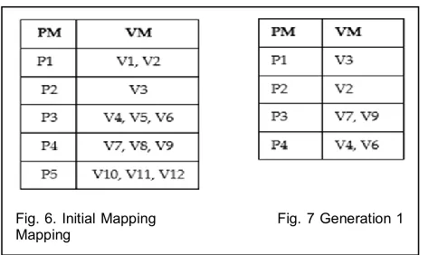
6.1.3 Selection Score

The Selection score is the criteria used in the algorithms which we have implemented, to allocate a VM to a Physical Server. This allocation of VM to a Physical Server happens sequentially and the selection score determines the order of VMs for allocation.

Selection Score =

VMs are selected in decreasing order of their selection score for allocation, i.e. VMs with higher characteristic costs are selected first. If we compute the Selection probabilities of all the VMs as described above, it shall add up to 1 as Illustrated for 5 VMs in Figure 4 below.

6.1.4 Fitness

The algorithms described in the later sections generate several solutions. Each solution contains VM-PM mappings for all VMs. The fitness of a solution is the predicted energy cost of running a job when VMs are allocated to the PMs as in the VM-PM mappings of the solution. We have used the PlanetLab workload to represent a typical Job and use that for computing the cost for identifying fitness.

6.2 Genetic Algorithm Adaptation

The adaptation of the Genetic Algorithm to our problem involves representing the problem and mapping probable solutions to the problem, as the population representation in the problem space. Then the fitness function is applied for each of these probable solutions and 10% of these are identified as the most probable solution. The next generation is generated by Mutating the VM-PM mapping, and then Migrate using a cross over as described below. We evaluate these probable solutions for fitness and choose 10% of this most probable solution. We do this for 3 generations. We then look at all the 3 generations of most probable solutions and pick the fittest solution as a global minimum for scheduling the VM into. The following sub-sections describe our implementation of a genetic algorithm.

6.2.1 Population Representation

The population for our problem space consists of several potential solutions i.e. mapping of VMs to servers as discussed in VM-PM mapping.

6.2.2 Population Initialization

Initialization would be to form the initial population, which is to generate the initial set of mapping of VMs to hosts, using the selection score as discussed above. As part of initialization, each of the copies of the VM to be scheduled, based on the Availability requirement, is scheduled into different Failure zones as discussed earlier. The selection of the VM for scheduling to a PM is based on a combination of the cumulative selection probability score as shown below in Table 3, and a Random number generated between 1-100.

The VM corresponding to the matching random number range in the table is chosen. This VM is mapped to the Physical Server with the lowest allocable capacity. This is randomized but increases the probability of the best-fit mapping as part of the initialization and preps it for energy efficiency. The table is then rewritten for 4 VMs and the process repeats. If there are not enough resources as required for the VM in the Physical Server, this same process is followed for other available Physical Servers.

Fig. 3.VM – PM Mapping

Fig. 4. Selection Score

1715 6.2.3 Crossover

Consider Physical Servers P1, P2, P3, P4 and P5 and VMs V1 to V12. The initial mapping of this population is as in Fig 6

Consider that the individuals mapping P1-V1, P2-V3, P3-V4, P3-V6, P4-V7, and P4-V9 have been evaluated with the Fitness function and look to be the probable solutions. Then the crossover of mappings is done and the Generation 1 population is generated as in Fig 7. The resultant mapping is feasible if the hosts can allocate their mapped VMs. These feasible mappings are evaluated by the Fitness function for fitness to be a probable solution. This process continues until the planned number of generations we want to consider is completed or until we have no new potential Mapping solution. We look at all the possible solutions across the generations and pick the one with the best fitness

6.2.4 Mutation

A VM is chosen at random such that it is the only VM assigned to its Physical Server. If there is no such VM, any VM is chosen at random. This VM is unassigned from its initial VM and reassigned to a random server that meets the VM‘s requirements and preferably already has another VM assigned to it.

6.2.5 Mutation

A VM is chosen at random such that it is the only VM assigned to its Physical Server. If there is no such VM, any VM is chosen at random. This VM is unassigned from its initial VM and reassigned to a random server that meets the VM‘s requirements and preferably already has another VM assigned to it.

6.2.6 Heuristics Employed

 We have employed representations like VM-PM mapping. We have also used customized operands like VM Characteristics Cost, Selection Score, Selection Probability as part of representing our problem domain.

 The Genetic Algorithm is classically configured with a higher probability of recombination and a low probability of mutation. Our experimentation, as can be seen, does not bring in too much of mutation

 We have chosen the fitness-proportionate selection based on the characteristics cost and the cost of energy and thus it does not make it too greedy nor too random.

6.2.7 Availability

We have factored in Adaptation of the Genetic Algorithm as seen above factors in Availability where the VM replicas as needed for the QoS Availability are associated with different

Failure Zones and the scheduling of the VMs further to this happens within the Failure zones. This ensures that VM copies are not scheduled into the same Failure zones thus reducing the probability of failures and increasing Availability.

6.2.8 Pseudo Code

for r=0 to numberOfReplicas in a failure zone { population = []

for i = 0 to populationSize: individual = generateIndividual() addToPopulation(individual) for i = 0 to numGenerations:

population = chooseNFittest (population, n) population = population + mutation(population) population = population + crossover(population) return chooseFittest(population)}

6.3 Particle Swarm Optimization

The adaptation of the PSO algorithm would need us to represent a particle into the problem space, and then consider possible solutions as the population representation in the problem space. We then compute the fitness value for all of the particles of the swarm, for that position using a fitness function and find the fittest mapping for that position which is the pBest. If there exists a global best (gBest) solution across all particles and positions, we compare and keep the fittest into the global position. We move the particle influenced by its pBest, the gBest, and random orientation, a predetermined number of times, and finally, identify the globally best position. This movement would be based on the goal of either to explore or exploitation of the current position.

6.3.1 Population Representation

Each particle in the PSO represents a solution for VM provisioning into a server, i.e. mapping of VMs to servers. The population in this swarm consists of several particles. These mappings consist of one to many relationships between servers and VMs.

6.3.2 Population Initialization

Initialization would be to form the initial population, which is to generate the initial set of mapping of VMs to hosts and as part of initialization, each of the copies of the VM to be scheduled, based on the Availability requirement, is scheduled into different Failure zones. The VMs and the PMs for mapping are based on a combination of the cumulative selection using the selection score as discussed earlier and similar to the Genetic Algorithm above in Fig 5. The selection of the VM is based on a combination of the cumulative selection probability score as shown below in Figure 6, and a Random number generated between 1-100. The VM corresponding to the matching random number range in the table is chosen. This VM is mapped to the Physical Server with the lowest allocable capacity. This is randomized but increases the probability of the best-fit mapping as part of the initialization and preps it for energy efficiency. The table is then rewritten for 4 VMs and the process repeats. If there are not enough resources as required for the VM in the Physical Server, this same process is followed for other available Physical Servers.

1716 6.3.3 Identification and registration of the Particle best

and the Global best

Post initialization, the fitness of each of the initialized mappings is evaluated using the fitness function which looks at the energy characteristic, and the fittest among them is stored as pBest along with its position. This is also stored as gBest during initialization. The position of the particles has moved a step using a velocity that is influenced by the current pBest, the gBest and a random factor. The new pBest and gBest are computed and stored as above. This process is repeated a predetermined number of times and post every step, the pBest and gBest are updated while the velocity of the particle values. At the end of a predetermined number of steps, the gBest arrived at is the candidate for the placement.

6.3.4 Velocity and Positional Updates

Once several particles are generated to form the initial population, each of the particles will move or undergo modifications in their VM-Host mapping. This is supported by providing a velocity to the particle and considering their position updates. Velocity is the number of hosts by which a VM jumps in a step.

The velocity of a particle in the (t + 1) th step is given by the equation:

v(t+1) = v(t) + c1 * rand( ) * (pBest(t) – x(t)) + c2 * rand() *

(gBest(t) – x(t)) (a)

where,

v(t + 1) is the velocity of particle in (t + 1)th step, v(t) is the velocity of particle in t‘th step,

c1 and c2 are acceleration coefficients, rand() is a random number in range [0, 1], x(t) is the position of particle in t‘th step,

gBest(t) is the position of the fittest particle across all generations until generation t,

pBest(t) is the position of a particle across its generations when it has been its fittest.

The position of a particle is moved by delta when moved in a step with the Velocity as above. This delta is added to the position of a particle in the current generation to get its position in the next generation. This position update is given by the equation:

x(t+1) = x(t) + v(t+1) (b) These equations (a) and (b) are used for determining the distance moved in the step and the position after the step.

6.3.5 Availability

Adaptation of the PSO Algorithm as seen above factors in Availability where the VM replicas as needed for the QoS Availability are associated with different Failure Zones and the scheduling of the VMs further to this happens within the Failure zones. This ensures that VM copies are not scheduled into the same Failure zones thus reducing the probability of failures and increasing Availability.

6.3.6 Pseudo Code

3.3 Energy consumption states of HDDs

6.3.7 Advantages of PSO

 PSO algorithms converge faster and have a higher probability and efficiency in finding the global optimum.

 The shorter computational time for running the algorithm

 It has fewer parameters to adjust, unlike many other competing evolutionary techniques. There are no crossover and mutation operators in GA and evolutionary programming.

7 E

S

A

W

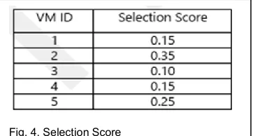
CloudSim a popular simulation framework for cloud environments as presented by Calheiros et al [8] has been used. CloudSim is an event-driven simulation framework where entities communicate with each other using a message passing mechanism. Entities in CloudSim are abstracted away as SimEntities, where each possesses its event queue and

1717 triggers for simulation of events. Events themselves are

abstracted away in a class called SimEvent. CloudSim also features classes for Hosts and VMsand supports time or space sharing VM scheduling policies. VMs themselves comprise of multiple Cloudlets representing a single task from the given workload. In the normal execution scenario of CloudSim simulation, Datacenter and Datacenter-Broker SimEntities are first created as can be seen in Figure 7. Each Data Center entity represents a user-specified configuration of Hosts and has associated classes for representing networking and storage. Datacenter broker sets-up the Data Center policies such as a VM allocation policy and number of VMs, as well as hands-off cloudlets from the workload to the datacenter for execution. Hosts in the Data Center has an associated power model which the Data Center entity uses to calculate its total energy consumption. Once the workload has finished running, the Data Center entity reports back to the broker with the simulation termination.

7.2 Setup

The following configurations in terms of the number of jobs, number, and types of host servers, VMs and replication factors were used as part of the Simulations.

 Simulation period – 3 hours

 Number of hosts – 2000

 4 VM types with configurations {CPUs, MIPS, RAM} = {1, 1000, 512 MB}, {2, 1500, 768 MB}, {2, 2000, 1536 MB}, {1, 2500, 1536 MB}

 2 host types with configurations {CPUs, MIPS, RAM} = {2, 5000, 4096 MB}, {2, 7500, 8192 MB}

7.3 Workload

All of these have been run with the PlanetLab workload which consists of CPU utilization traces from PlanetLab VMs collected during 10 random days in March and April 2011. We have chosen 3 hours of data of one day from the dataset. Since each job type has near constant CPU and memory allocations, as well as a near-constant number of running tasks, and we have considered each job to be an individual application.

We have also verified the results by running with Google Cluster Workload.

8 S

A

R

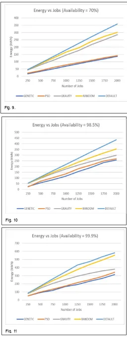
Simulation of the baselined algorithms with our adapted nature-inspired Genetic and PSO algorithm has been performed using the CloudSim infrastructure. This involved Workloads which were run with ~2000 Jobs with two Availability requirements 70% (Figure 9), 98.5% (Figure 10) and 99.9% (Figure 11) which are mapped to having 1, 2 and 3 replicas.

Fig. 9.

Fig. 10

1718 The above results of simulation running 2000 jobs for different

levels of availability for different algorithms. It can be seen that the energy consumption increases for increasing availability

The experimentation results (Figures 12, 13 and 14) also show that there is an increase in the time taken for finding the best physical machine to map on to increases with the number of jobs as expected and varies significantly as can be seen for

different Algorithms with different Availability percentages. The results also show that PSO and the Genetic Algorithms consume significantly higher time to find the right fit as compared to the Gravity Algorithm. This time also increases with the QoS Availability expectations along with the number of replications.

9 C

It can be concluded that Genetic and PSO Algorithms perform better than the default, random and Gravity algorithms in terms of power consumption or Energy efficiencies with Availability consideration. The other observation which can be made is, the total energy consumed expectedly increases with an increase in the Availability expectations due to the larger number of servers running in multiple failure zones. The computational overhead for both Genetic and PSO Algorithms is high and hence there is more latency involved in scheduling using these Algorithms when compared with the Gravity, Random and the default Algorithms. This is visible with the time taken by the algorithms to arrive at the best fit. So, we can conclude that a lightweight approach like Gravity algorithm provides a good trade-off between the different algorithms chosen for exploration for the given workload.

References

[1] Sitaram, Dinkar, H. L. Phalachandra, S. Gautham, H. V. Swathi, and T. P. Sagar. "Energy-efficient data center management under availability constraints." In Systems Conference (SysCon), 2015 9th Annual IEEE International, pp. 377-381. IEEE, 2015.

[2] Ghribi, Chaima, Makhlouf Hadji, and Djamal Zeghlache. "Energy-efficient VM scheduling for cloud Data Centers: Exact allocation and migration algorithms." In Cluster, Cloud and Grid Computing (CCGrid), 2013 13th IEEE/ACM International Symposium on, pp. 671-678. IEEE, 2013.

[3] Lin, Ching-Chi, Pangfeng Liu, and Jan-Jan Wu. "Energy-aware virtual machine dynamic provision and scheduling for cloud computing." In 2011 IEEE 4th International Conference on Cloud Computing, pp. 736-737. IEEE, 2011.

[4] Buyya, Rajkumar, Rajiv Ranjan, and Rodrigo N. Calheiros. "Modeling and simulation of scalable Cloud computing environments and the CloudSim toolkit: Challenges and opportunities." In High-Performance Computing & Simulation, 2009.

[5] Calheiros, Rodrigo N., Rajiv Ranjan, Anton Beloglazov, César AF De Rose, and Rajkumar Buyya. "CloudSim: a toolkit for modeling and simulation of cloud computing environments and evaluation of resource provisioning algorithms." Software: Practice and experience 41, no. 1 (2011): 23-50

[6] Wickremasinghe, Bhathiya, Rodrigo N. Calheiros, and Rajkumar Buyya."CloudAnalyst: A Cloudsim-based visual modeler for analyzing cloud computing environments and applications." In Advanced Information Networking and Applications (AINA), 2010 24th IEEE International Conference on, pp. 446-452. IEEE, 2010

[7] Zhang, Xinqian, Tingming Wu, Mingsong Chen, Tongquan Wei, Junlong Zhou, Shiyan Hu, and Rajkumar Buyya. "Energy-aware virtual machine allocation for the cloud with resource reservation." Journal of Systems and Software 147 (2019): 147-161.

[8] Kliazovich, D., Bouvry, P. and Khan, S.U., 2013. DENS: Data Center energy-efficient network-aware scheduling. Cluster computing, 16(1), pp.65-75.

Fig. 12

Fig. 13

1719 [9] Buyya, R., Beloglazov, A. and Abawajy, J., 2010. Energy-efficient

Management of Data Center resources for cloud computing: a vision, architectural elements, and open challenges. arXiv preprint arXiv:1006.0308

[10]Garg, S.K., Yeo, C.S. and Buyya, R., 2011, August. Green cloud framework for improving the carbon efficiency of clouds. In European Conference on Parallel Processing (pp. 491-502). Springer, Berlin, Heidelberg.

[11]Fayyaz, A., Khan, M.U., and Khan, S.U., 2015, December. Energy-efficient resource scheduling through VM consolidation in cloud computing. In 2015 13th International Conference on Frontiers of Information Technology (FIT) (pp. 65-70). IEEE. [12]Heller, B., Seetharaman, S., Mahadevan, P., Yiakoumis, Y.,

Sharma, P., Banerjee, S. and McKeown, N., 2010, April. Elastictree: Saving energy in Data Center networks. In NSDI (Vol. 10, pp. 249-264).

[13]Kliazovich, D., Bouvry, P. and Khan, S.U., 2012. GreenCloud: a packet-level simulator of energy-aware cloud computing Data Centers. The Journal of Supercomputing, 62(3), pp.1263-1283. [14]Fang, W., Liang, X., Li, S., Chiaraviglio, L. and Xiong, N., 2013.

VMPlanner: Optimizing virtual machine placement and traffic flow routing to reduce network power costs in Cloud Data Centers. Computer Networks, 57(1), pp.179-196.

[15]Combarro, M., Tchernykh, A., Kliazovich, D., Drozdov, A. and Radchenko, G., 2016, November. Energy-aware scheduling with computing and data consolidation balance in 3-tier Data Center. In 2016 International Conference on Engineering and Telecommunication (EnT) (pp. 29-33). IEEE.

[16]Moore, J.D., Chase, J.S., Ranganathan, P. and Sharma, R.K., 2005, April. Making Scheduling‖ Cool‖: Temperature-Aware Workload Placement in Data Centers. In USENIX annual technical conference, General Track (pp. 61-75).

[17]Cao, T., Huang, W., He, Y. and Kondo, M., 2017, May. Cooling-aware job scheduling and node allocation for overprovisioned HPC systems. In 2017 IEEE International Parallel and Distributed Processing Symposium (IPDPS) (pp. 728-737). IEEE

[18]Phalachandra HL, Priyank Bhandia, Ravi S. Anupindi, Pavan Yekbote, Nikhil Singh, Dinkar Sitaram, 2019 February, DCSim: Cooling Energy-Aware VM Allocation Framework for Cloud Data Center, In 2019 International Conference on Advances in Computing & Communication Engineering (ICACCE-2019), IEEE

[19]Vishwanath, Kashi Venkatesh, and Nachiappan Nagappan. "Characterizing cloud computing hardware reliability." In Proceedings of the 1st ACM symposium on Cloud computing, pp. 193-204. ACM, 2010.

[20]Failure Rates in Google Data Centers [https://www.datacenterknowledge.com/archives/2008/05/30/fail ure-rates-in-google-data-centers]

[21]Mao, M., Li, J. and Humphrey, M., 2010, October. Cloud auto-scaling with a deadline and budget constraints. In 2010 11th IEEE/ACM International Conference on Grid Computing (pp. 41-48). IEEE.

[22]Chen, Y., Wang, Q.B., Xiang, Z. and Yang, B. 2013. ―Method and Apparatus of Dynamically Allocating Resources across Multiple Virtual Machines.‖

[23]Liu, Haikun, et al. 2011. Performance and Energy Modeling for Live Migration of Virtual Machines.

[24]W. Wang and H. Chen, ―An availability-aware virtual machine placement approach for dynamic scaling of cloud applications,‖ in IEEE 9th International Conference on Ubiquitous Intelligence and Computing, 2012, pp. 509–516.

[25]J. Yang, C. Liu, Y. Shang, Z. Mao, and J. Chen, ―Workload Predicting-Based Automatic Scaling in Service Clouds,‖ 2013. [26]M. Jammal, A. Kanso, and A. Shami, ―CHASE: Component