DEPENDABLE FLOW ANALYSIS IN LEMATANG WEIR

1626

DEPENDABLE FLOW ANALYSIS

IN LEMATANG WEIR

Bambang Milianto, Anis Saggaff, Febrian Hadinata

Abstract— Water resources are needed currently very much, especially in the area of Kota Pagar Alam for the purposes of rice fields which are planned to be served by Lematang Weir. The purpose of this study is to determine water availability to calculate dependable flow in Lematang Weir by using the Hydrology Engineering Center-Hydrologic Modeling System (HEC-HMS) model. The Lematang Weir watershed is influenced by land cover and average monthly rainfall which ranges from 7.13 mm in 2018, based on rainfall data which is taken from satellite rainfall data (TRMM). Based on mapping analysis and Geographical Information System (GIS) software, the Lematang Weir watershed is obtained covers an area is 59.889 km2. By using HEC-HMS software, the simulation results to show that the Q80 dependable flow in the Lematang Weir watershed is 1 m3/s and Q90 is 0.70 m3/s.

Index Terms— Watershed, dependable flow, HEC-HMS, hydrology, water availability, Q80, TRMM.

——————————  ——————————

1

I

Water is an important resource for life sustainability and water accessibility is a very significant factor in the sustainable development of humans. Climate change, population, and land use have a deep impact on the future supply and demand for water resources in the future and global water availability and regional scale [1]. Watershed is one part of hydrology, Watershed also has the function of transforming from the form of rainfall input into other elements such as sediment, nutrients etc [2]. Water flow in a watershed depends on the amount of rainfall, rainfall intensity, catchment area characteristics, soil type, soil conditions and surface impermeability [3]. Information on how much flow discharge is available from a water source can be obtained from recorded river flow discharges or from high rainfall data recorded at a rainfall station. High rainfall data can be used when have time keeping to recorded [4]. Flow discharge is the total of all surface runoff, rainfall that falls directly in the river, streams around the river, and riverbed flow [5]. If the analysis of water availability uses high rainfall data, the next step is to change the high rainfall data for a station (rainfall point station) to be the high rainfall area (rainfall area). The final step in the analysis of water availability is to determine the dependable flow as the design value of the discharge from the monthly average [6]. Rainfall is one of the elements climate that has a high variation in the scale of space although time so that is difficult to predict. The degree of difficulty is getting lower after is found out some reliable rainfll data analysis techniques. However, this reliable analytical technique often requires the availability of complete observational rainfall data, ie the recording period is continuous and the number of staking stations represents the condition of the area being measured. This condition is not yet fully in the Lematang watershed. One of the ways to overcome this problem is to use simulated or conjecture rainfall data which is obtained from weather satellites such as TRMM rainfall data [7]. The limited data on a river will reduce the reliability of water potential in a river. Therefore, an analysis is needed to determine the availability of data in a river. One of analysis is used the rainfall runoff (R-R) analysis. In this study the R-R model that will be used is the HEC-HMS (Hydrology

Engineering Center-Hydrology Modeling System) software. The deterministic distributed hydrological model of HEC-HMS is used to simulate flow in watershed hydrological units. HEC-HMS is decided as a software-based tool to simulate the hydrological cycle in the context of problem solving techniques [8].

2 M

In general, this research is undertaken in 3 stages, i.e. correction of satellite rainfall data, determination of model parameters through model calibration and dependable flow calculation. Satellite rainfall data from TRMM will be corrected with existing data. This correction is needed to determine the impact of meteorology and the actual topographical conditions. The advantages of remote sensing technology should be further utilized to study the characteristics of weather and climate in an area for the benefit of water resource management and its utilization for the welfare of the community [9]. Specifically for the tropics area, a remote sensing device is currently available which undertaken rainfall measurement missions in the tropics area using the TRMM (Tropical Rainfall Measurement Mission) satellite. TRMM is a space cooperation project between NASA and the Japan Aerospace Exploration Agency (JAXA) which is intended to monitor and study rainfall in the tropics area in the context of NASA's long-term effort to study the earth as a global system [10]. Since it was published in 1998, TRMM data has been widely used in various studies of weather and climate problems in Indonesia, such as the use of TRMM satellite data for studies of extreme weather conditions [11]. Comparison of monthly rainfall based on observations by TRMM satellites and NOAH surface models, the results are TRMM data has the potential to fill temporally blank surface data for a location and spatial vacancy for areas that have less surface rainfall observation density [12]. TRMM produces estimates of rainfall for various monitoring activities. TRMM is equipped with three sensors i.e PR (Precipitation Radar), TMI (TRMM Microwave Imager), and VIRS (Visible and Infrared Scanner). TRMM data is able to measure daily three-to-monthly rain in a 0.25° or 27 km. After correction of satellite rainfall data, the model parameters are determined through model calibration using HMS software. The hydrological model with the HEC-HMS program is designed to simulate the rainfall-runoff process of a flow system. This program is designed to be applied in a certain area to represent the watershed hydrological process [13]. Several studies have been undertaken by using the HEC-HMS model in various regions with different soil and climatic conditions, by using the

HEC-————————————————

 Bambang Milianto is master student in Civil Engineering, Faculty of Engineering, Sriwijaya University, Indonesia. Corresponding Email: [email protected]

 Anis Saggaff, Civil Engineering Department, Faculty of Engineering, Sriwijaya University, Indonesia.

HMS model for both occasion and sustainable hydrological modeling in the Monalack watershed in western Michigan [14].

3 R

D

3.1 Satellite Data Correction

Before making corrections to satellite data, it must be known the distribution of rainfall data and discharge data availability at the study location.

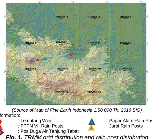
(Source of Map of Fine Earth Indonesia 1:50.000 Th. 2016 BIG)

Information:

: Lematang Weir : Pagar Alam Rain Posts : PTPN VII Rain Posts : Jarai Rain Posts

: Pos Duga Air Tanjung Tebat

Fig. 1. TRMM grid distribution and rain post distribution

Based on the map identification, it is known that there are 4 rainfall station in the Lematang weir watershed managed by the Climatology and Geophysics Meteorological Agency, and BPSDA Musi including Pagar Alam Rain Posts, Jarai, PTPN VII, and Tanjung Tebat/Pulau Pinang. In addition, there are also 2 water conjectures station located downstream of the watershed, i.e. the Lematang-Lebak Budi water conjectures station and Lematang-Pinang Belarik. Both of these water conjectures station are needed for using the calibration process of the R-R model. Based on existing ground station data, only PTPN VII rainfall sration and Jarai rainfall station are able to correct data from TRMM due to there are more data available than other rainfall station.

3.2 Topographic Characteristics for Modeling Parameter Selection

Based on mapping analysis and Geographic Information System (GIS) software, it is found that the Lematang weir watershed is 59.889 km2, due to the model scheme which is used up to downstream, the study watershed is 3.857 km2.

Fig. 2. Land use in the study basin

(Source of Map of Fine Earth Indonesia 1:50.000 Th. 2016 BIG)

Information:

: Lematang Weir : Plantation/Garden : Body Of Water : Paddy Field : Jungle / Forest : Shurbs

Fig. 3. Land use map

For land cover in the study watershed 45.03% are plantations, 26.5% of the forest and the rest are in the form of rice fields, shrubs and others. The watershed land use resume can be seen in Fig. 2. By seeing the condition of the land use distribution above, in general the condition of the watershed is still in good condition. The following is a map of land use distribution for the study area.

3.3 Modeling of Rainfall

The model is used in the local inflow analysis is the Hydrologic Engineering Center-Hydrologic Modeling System (HEC-HMS) software. The HEC-HMS model has been widely used as a runoff rain model with satisfactory calibration results in various studies [15]. By using the model for the hydrological study and analysis of the Krueng Langsa river form capacity. Hydrological simulations are based on rainfall data for a 2-year return period plan. Flood discharge is obtained to use HEC-HMS software is 59.30 m³/sec. This value approaches the discharge value by passing capacity analysis on the river cross section, which is 60.07 m³/sec, this was done on the prediction of supply and water needs of the Ciliwung River in the Panus to Manggarai bridge sections [16]. This model divides the watershed into small sub-watersheds. Based on GIS analysis, the study watershed is divided into 70 small sub-watersheds with a scheme as shown in Fig. 4. Due to the

1628

unavailability of hourly discharge data, data calibration is performed by using the daily discharge data.

The parameters which is calibrated in this model are: 1. A deficit constant parameter that describes the amount of

water that passes to become infiltration.

2. Transform parameters that describe the time is needed for rainfall to the ground surface to become a surface flow. 3. Baseflow parameters that describe river bed flow

characteristics.

Fig. 4. Rainfall mode scheme – watershed study using

HEC-HMS of HEC-HEC-HMS at the water forecast post of Lematang-Lebak Budi

Table 3 through Table 4 are the hydrological parameters is used in the model.

Calibration calculations are undertaken to use the parameters above to find the smallest absolute error so that the result calculation discharge approaches the observation flow discharge. Calibration was undertaken at the Lematang-Lebak Budi at conjecture station in the 1999 data, due to the data is used were quite feasible. The feasibility of the conjecture station data of the Lematang-Lebak Budi water is due to several things, i.e. the discharge curve is used and the form of daily hydrograph in 1 year. The following is a resume of the publication of discharge data based on the measurement of the discharge (making a discharge curve).

Table 1. Debit curve resume used

No. Water Forecast Post

Discharge data Publication

Discharge measurements years

(Discharge Curve) 1 Lematang-Lebak

Budi

1998-1999 2004-2008

2009

1991-1998

2 Lematang-Pinang Belarik

1998 2004-2007

1990-1999 2000-2003

Based on resumes in Table 1, the data that can be used is between 1998-1999 due to the discharge curve is used to convert daily water levels in the year are the result of discharge measurements made from 1991-1998 for the conjecture station Lematang-Lebak Budi and discharge measurements in 1990-1999 for the conjecture station Lematang-Pinang Belarik. Whereas for other year discharge like the table above, it can be seen that the publication of the 2004-2009 used the discharge curve of the measurement results 1998-1999 in other words the conversion of the

discharge data is doubtful because the cross section conditions at that time are not in accordance with the actual cross section conditions, take into consideration the river in

Indonesia is strongly influenced by crushing and

sedimentation. Calibration is used to determine the closeness between the value of the simulation model generated to the observation discharge data is obtained from the field. In addition to graphic form, the closeness can also be seen from the Nash-Sutcliffe coefficient (NSE) value. The following categories of model reliability are based on these coefficient values.

Table 2. NSE value range for the reliability level of the hydrological model

Goodness of fit NSE

Very good NSE>0,6

Goodness of fit 0,40<NSE≤0,60 Satisfactory 0,20<NSE≤0,40 Unsatisfactory NSE<0,20

Note : E: Nash-Sutcliffe coefficient, RRSE: root relative squared error, PBIAS: bias percentage (Sumber: Pérez-Sánchez, dkk (2017))

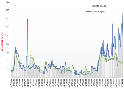
The results of calibration is undertaken by trial and error produce a satisfactory NSE value i.e 0.328. These results have been very good looking at the observation data which is a bit dubious in the last months of the year. This calibration can be seen in Fig. 5.

Fig. 5. Calibration of the rain flow model at the Air Lematang-Lebak Budi post

Table 3. Constant deficit parameters for the study watershed

Sub DAS

Initial deficit (mm)

Max storage (mm)

Constant rate (mm/hr)

W2270 0.6 49.22 1.27

W2280 0.6 61.77 1.27

W2290 0.6 67.71 1.27

W2300 0.6 41.76 1.27

W2310 0.6 63.67 1.27

W2320 0.6 30.26 1.27

W2330 0.6 36.02 1.27

W2340 0.6 60.95 1.27

W2350 0.6 63.54 1.27

W2390 0.6 41.29 1.27

W2430 0.6 59.61 1.27

W2440 0.6 52.85 1.27

W2450 0.6 56.54 1.27

W2460 0.6 60.38 1.27

W2490 0.6 52.26 1.27

Sub DAS

Initial deficit (mm)

Max storage (mm)

Constant rate (mm/hr)

W2550 0.6 38.08 1.27

W4270 0.6 132.65 3.81

W4290 0.6 115.12 3.81

W4440 0.6 140.22 3.81

W4520 0.6 103.75 3.81

W4530 0.6 145.26 3.81

W4570 0.6 69.32 1.27

W4580 0.6 94.21 3.81

W4630 0.6 87.20 3.81

W4670 0.6 51.70 1.27

W4680 0.6 44.75 1.27

W4720 0.6 43.49 1.27

W4730 0.6 40.67 0

W4780 0.6 57.35 1.27

W4820 0.6 63.94 1.27

W4830 0.6 67.71 1.27

W4870 0.6 42.40 3.81

W4880 0.6 57.64 3.81

W4270 0.6 132.65 3.81

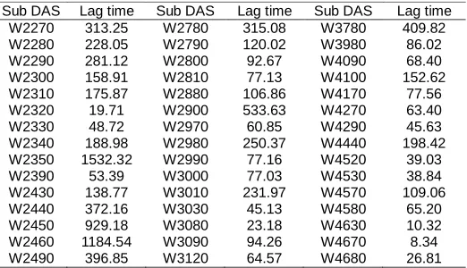
This loss method is able to calculate continuous rainfall loss to become runoff. This method is influenced by soil type and humidity. The loss parameter is used in this analysis ie. the Maximum Storage which is the capacity of the sub-watershed, while the Constant rate is the rate of water absorbed and stored in the soil due to the infiltration process. The following is the loss parameters generated based on the calibration results. This transform method is used to calculate the length of time the rainfall changes to become runoff. This parameter is explicitly determined by the Lag Time parameter which depends on length, slope, cross section of the channel and river and roughness coefficient. The grace period for this parameter can be estimated by calibration, for those who have observational data at the conjecture station. In cases where there is no data, suggest a grace period is estimated from the time of concentration tc through the formula tlag = 0.6 tc.

Whereas the concentration time is estimated from the formula:

t = tsheet + tshallow + tchannel (1)

where:

tsheet is the amount of travel time of a layer or sheet flow

segment above ground level, tshallow is the amount of travel time

of shallow flow on the road, gutters, soil grooves and tchannel is

the amount of travel time of the channel or river. For river flow, is needed cross-sectional, cross-sectional data and velocity estimates by using Manning formula n. Following is the lag time value for each sub-watershed.

Table 4. Input parameter transform for study watershed

Sub DAS Lag time Sub DAS Lag time Sub DAS Lag time W2270 313.25 W2780 315.08 W3780 409.82 W2280 228.05 W2790 120.02 W3980 86.02 W2290 281.12 W2800 92.67 W4090 68.40 W2300 158.91 W2810 77.13 W4100 152.62 W2310 175.87 W2880 106.86 W4170 77.56 W2320 19.71 W2900 533.63 W4270 63.40 W2330 48.72 W2970 60.85 W4290 45.63 W2340 188.98 W2980 250.37 W4440 198.42 W2350 1532.32 W2990 77.16 W4520 39.03 W2390 53.39 W3000 77.03 W4530 38.84 W2430 138.77 W3010 231.97 W4570 109.06 W2440 372.16 W3030 45.13 W4580 65.20 W2450 929.18 W3080 23.18 W4630 10.32 W2460 1184.54 W3090 94.26 W4670 8.34 W2490 396.85 W3120 64.57 W4680 26.81

Sub DAS Lag time Sub DAS Lag time Sub DAS Lag time W2530 85.64 W3150 163.62 W4720 191.73 W2550 202.20 W3170 116.19 W4730 49.76 W2570 70.42 W3220 326.90 W4780 60.42 W2610 164.40 W3340 132.38 W4820 59.15 W2670 406.18 W3360 297.04 W4830 28.19 W2680 78.30 W3370 51.81 W4870 65.63 W2710 19.47 W3450 224.91 W4880 193.93 W2720 92.27 W3530 332.37

W2730 36.05 W3620 289.28

The Baseflow method is used to determine the shape and magnitude of the baseflow that each Sub-Watershed has. This method uses linear reservoir parameters to simulate base flow after rain stops. Previously calculated infiltration acts as an inflow for a linear reservoir. This method can use one or two layers with 50% and 50% division. There are 6 parameters in the method, i.e.: Groundwater 1 has three parameters: initial conditions (m3/s/km2), reservoir reservoir coefficient (hours), number of reservoirs and groundwater layer 2: initial conditions (m3/s/km2), reservoir storage coefficient (hours), number of reservoirs. The initial conditions illustrate the contribution of base flow from the first and second layers of groundwater. Reservoir storage coefficient is the time of water storage in reservoirs in each layer due to it is calculated in hours it will give meaning to the response time of the sub-watershed. The number of groundwater reservoirs illustrates the search for basic flow through several series of reservoirs. Reducing the base flow discharge in each reservoir means that more reservoirs reduce so the effect more discharge is getting decrease. The calibration results show the parameters as follows:

GW 1 initial is 0.008 m3/s/km2 GW 1 coefficient is 110 hours GW 1 reservoir as much as 1 GW 2 initial is 0.008 m3/s/km2 GW 2 coefficient is 275 hours GW 2 reservoir as much as 2

If the discharge data is available, the dependable flow calculation can be done by following SNI No. 6738: 2015 concerning calculation of dependable flow with a discharge duration curve. The formula is used in the calculation of the dependable flow by using frequency method is as follows.

(2)

Where:

P(X<x) = probability of the occurrence of variable X (flow discharge) that is greater than x (m3/s)

m = data rank

n = the amount of data

X = a discharge data series

1630

Fig. 6. The duration curve of Lematang weir flow

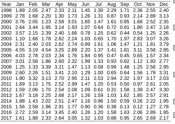
The following is the result of the calculation of flood discharge that has been done which can be seen in Fig. 9 that produces a resume of peak flood of the weir using the HSS Gamma 1 method. Based on the results of calculations that have been made, the resulting Q80 is 1 m3/s, Q95 is 0.40 m3/s, and Q98 is 0.3 m3/s. While the average monthly discharge that occurs at Lematang weir can be seen below.

Table 5. Input parameter transform for study watershed

Year Jan Feb Mar Apr May Jun Jul Aug Sep Oct Nov Dec 1998 1.89 2.05 2.47 2.33 2.11 1.45 1.30 2.29 1.71 2.36 2.55 2.40 1999 2.78 1.68 2.20 1.30 1.73 1.26 1.31 0.87 0.93 2.14 2.89 3.13 2000 3.76 2.05 1.23 2.58 3.01 1.65 1.47 1.61 0.85 1.68 2.52 2.35 2001 2.64 3.44 1.95 3.14 1.93 1.07 0.64 0.72 0.81 1.80 2.47 2.18 2002 3.57 2.15 2.39 2.40 1.66 0.78 1.25 0.62 0.44 0.54 1.25 2.26 2003 1.10 1.68 1.78 2.62 2.24 1.03 0.65 1.70 1.97 2.83 3.07 3.26 2004 2.31 2.40 2.03 2.62 2.74 0.99 1.61 1.06 1.47 1.21 1.81 3.79 2005 4.55 3.19 4.54 3.25 2.89 2.20 1.37 1.41 1.81 3.11 3.58 2.85 2006 4.03 2.78 2.03 2.34 1.76 1.84 0.95 0.47 0.45 0.65 1.57 2.34 2007 3.01 2.58 1.86 2.60 2.32 1.99 1.33 0.93 0.82 1.12 1.93 2.77 2008 1.25 1.33 3.39 3.21 1.47 1.13 0.58 0.99 1.48 1.25 2.56 2.95 2009 2.60 2.26 1.51 3.41 2.10 1.29 1.00 0.65 0.64 1.56 1.78 3.31 2010 1.80 3.32 3.13 2.70 2.95 2.11 2.53 2.94 2.32 1.97 3.17 2.03 2011 1.69 3.13 1.75 2.52 2.99 1.47 1.20 0.53 0.50 0.97 2.61 2.05 2012 1.59 2.06 1.70 2.54 2.08 1.09 0.61 0.31 1.58 1.39 2.47 3.30 2013 1.67 3.18 2.25 2.68 2.17 1.26 1.59 1.03 1.62 1.85 2.57 2.91 2014 1.88 1.43 2.02 2.51 2.47 1.16 0.96 1.50 0.59 0.26 2.22 1.95 2015 1.56 2.58 1.96 2.91 1.77 0.90 0.36 0.38 0.13 0.12 1.27 2.78 2016 2.72 2.59 3.14 3.45 2.40 1.26 1.20 1.58 1.63 2.06 2.89 1.95 2017 1.61 1.88 2.33 2.64 3.05 1.32 1.03 0.88 0.95 2.65 2.69 2.17

4 C

1. Based on the results of research that has been done it can be concluded that the results of verification using groundstation rainfall data show an NSE value is 0.328. This shows that the runoff rain model formed is satisfactory. Simulation results shows that dependable flow Q80 in Lematang Weir watershed is 1 m3/s and Q90 is 0.70 m3/s.

2. From the analysis results above, it shows that TRMM satellite data can be used to replace incomplete rainfall data in a study area.

R

[1] Arnell, N., W., van Vuuren, D., P., & Isaac, M. ―The implications of climate policy for the impacts of climate

change on global water resources‖, Global Environmental Change, vol. 21, no. 2, pp. 592-603, May 2011.

[2] Seyhan, E. Dasar-Dasar Hidrologi, Yogyakarta : Gadjah Mada University Press, 1990.

[3] Willems, P., Arnbjerg-Nielsen, K., Olsson, J., & Nguyen, V. ―Climate change impact assessment on urban rainfall

extremes and urban drainage: methods and

shortcomings‖, Atmospheric research, vol. 103, pp. 106-118, Jan 2012.

[4] Chay, A. Hidrologi dan Pengelolaan Daerah Aliran Air Sungai: Edisi Revisi Kelima, Yogyakarta : Gadjah Mada University Press Yogyakarta, 2010.

[5] Tivianton, T., A, ―Analisis Hidrograf Banjir Rancangan terhadap Perubahan Penggunaanlahan dalam Berbagai Kala Ulang Metode Hujan-Limpasan dengan HEC-GeoHMS dan HEC-HMS (Studi Kasus: Daerah Aliran Sungai Garang, Provinsi Jawa Tengah),‖ Tesis Program Pascasarjana Universitas Gadjah Mada., 2008.

[6] Triatmodjo, B. Hidrologi Terapan, Yogyakarta : Beta Offset, 2016.

[7] Bambang Dwi Dasanto. ―Evaluasi Curah Hujan TRMM menggunakan Pendekatan Koreksi Bias Statistik‖, Jurnal Tanah dan Iklim, vol. 31, no. 1, 2014.

[8] Scharffenberg, W., Ely, P., Daly, S., Fleming, M., & Pak, J. ―Hydrologic Modeling System (HEC-HMS): Physically-Based Simulation Components‖, 2nd Joint Federal Interagency Conference, June 27-July 1, Las Vegas, NV, 2010.

[9] Syaifullah, M., D. ―Validasi Data TRMM Terhadap Data Curah Hujan Aktual di Tiga DAS di Indonesia‖, Jurnal Meteorologi dan Geofisika, vol. 15, no. 2, pp. 109-118, Nov 2014.

[10]NASDA. TRMM Data Users Handbook. Earth Observation Center, National Space Development Agency of Japan, 2001.

[11]Marpaung, S., Satiadi, D., & Harjana, T. ―Analisis Kejadian Curah Hujan Ekstrim di Pulau Sumatera Berbasis data Satelit TRMM dan Observasi Permukaan‖, Jurnal Sains Dirgantara, vol. 9, pp. 127-138 Juni 2012.

[12]Gunawan, D, ―Perbandingan Curah Hujan Bulanan Dari Data Pengamatan Permukaan, Satelit TRMM dan Model permukaan NOAH‖, Jurnal Meteorologi dan Geofisika, vol. 9, no.1, pp. 65-77 2008.

[13]US Army Corps of Engineers, Technical Reference Manual Hydrologic Modelling System, Washington, 2000. [14]Chu, X., & Steinman, A. ―Event and Continuous

Hydrologic Modeling with HEC-HMS‖, Journal of Irrigation And Drainage Engineering, vol. 135, no. 1, pp 119-124, Feb 2009.

[15]Ichsan, S. ―Kajian Hidrologi dan Analisa Kapasitas Tampang Sungai Krueng Langsa Berbasis HEC-HMS dan HEC-RAS‖. Universitas Abulyatama, Fakultas Teknik, Jurusan Teknik Sipil, 2015.

[16] Suprapto, M., Yohana, B., N., P, & Siti, Q. ―Prediksi Pasok