Review of background oriented schlieren and development for ballistic
range applications
Ardian B. Gojani1,a, Burim Kamishi2, and Shigeru Obayashi1
1 Institute of Fluid Science, Tohoku University, 2-1-1 Katahira, Aoba, 980-8577 Sendai, Japan
2 Department of Physics, Faculty of Mathematical and Natural Sciences, University of Prishtina, Mother Theresa str., nn, 10 000 Prishtina, Kosovo
Abstract. Quantitative measurements of fluid flow can be achieved by flow visualization techniques, and this paper reviews and outlines background oriented schlieren, with emphasis on its performance: measurement sen-sitivity and uncertainty. Since the technique depends on cross-correlation, an assessment of image evaluation is also conducted. Background oriented schlieren is applied to two flows: shock reflection from a wedge in a shock tube, and natural cooling by convection. It is estimated that the technique can be applied to ballistic facilities.
1 Introduction
The idea of developing a quiet supersonic transport aircraft based on the Busemann biplane relies on the fact that wave drag which appears during supersonic fligh – and conse-quently, the intensity of the sonic boom, – can be reduced by a clever combination of aircraft elements. Details can be found in the article 4.19 of Liepmann and Roshko’s book Elements of Gasdynamics, [1]. This concept is supported by theoretical considerations, as it historically originated and developed, and a wealth of numerical studies. A more recent parametric study is given in the work by Igra and Arad [2], and airfoil optimization in the work by Hu et al. [3]. A thorough numerical study with many references is presented in the Lecture Notes of Kusunose et al. [4].
The scarcity of experimental studies, on the other hand, is evidenced by the most recent review on the state of the study of supersonic biplane written by Kusunose et al. [5], where the only published experimental work on Busemann biplane prior to the ongoing work in Japan that started in mid 2000s, was conducted by A. Ferri, which was car-ried out in 1940s in a wind tunnel, and where aerodynamic forces were measured and flow visualization was done by using Toepler schlieren method. Applications of these two methods make the bulk of recent experiments, as well. Qual-itative flow characteristics, mainly the effect of shock wave – expansion wave interference, are obtained indirectly by using schlieren visualization on wind tunnels, and the re-sulting images are later compared to CFD calculations, [6– 9]. Smoke based visulaization in combination with force measurements has also been applied, with the aim to in-vestigate the biplane behaviour at liftoffor nondesign con-ditions, [9, 10]. The pressure distribution on the surface of the biplane has been experimentally measured by pres-sure and temperature sensitive paints, [7, 8, 11], and in the work of Saito et al. some boundary layer effects were ob-served. Concluding remarks common to all these exper-iments are that, in general, flow field matches well with CFD predictions, but quantitative 3D (even 2D)
measure-a e-mail:gojani@edge.ifs.tohoku.ac.jp
ments are still required, and that biplane model support-ing mechanisms in wind tunnels interefere with the overall flow. The second issue is addressed by experimenting with a free flight of a Busemann biplane model in a ballistic range, with schlieren visualization as the main diagnostic method, [12].
It is a normal development of this study to experimen-tally attempt quantitative flow field characterization in and around supersonic Busemann biplane. The closest to ideal measurements on a real model in free flight are measure-ments on a scaled model flying supersonically in a ballistic range. This experiment, then, requires the development of two independent tasks: (i) launching of the biplane model in a ballistic range facility, and (ii) measuring flow charac-teristics.
There is already a precedent with the first part, as re-ported by Toyoda et al. [12], while the ballistic range at IFS, Tohoku University is constantly used for launching projectiles up to hypersonic velocities. Thus, the operation of the ballistic range does not pose any challenges, if the model and flight conditions are provided.
For the measurement of flow characteristics, on the other hand, the best option lays with flow visualization. Direct temperature and pressure measurements by using gauges on a small model in a ballistic range are forbidingly dif-ficult, while alternative options of temperature measure-ments by using imaging and spectroscopic methods (for example, thermal imaging, laser induced fluorescence, etc.) usually end up being expensive and complicated. Within two types of flow visualization, as categorized by Merzkirch in [13], marker methods (smoke visualization, particle im-age velocimetry, molecular tagging velocimetry, oil drops, etc.) are not applicable for the problem at hand, because of the complicated interaction of the model’s flight and the seeded flow markers, or because they give only informa-tion about the flow properties on the surface of the wings. In optical flow visualization types of experiments (shadow-graph, schlieren, interferometry, speckle, etc.), light serves as thegaugeof the refractive index or its variation in the flow field, and by virtue of direct relationship between
re-DOI: 10.1051/
C
Owned by the authors, published by EDP Sciences, 2013 epjconf 201/ 34501034
This is an Open Access article distributed under the terms of the Creative Commons Attribution License 2 0 , which . permits unrestricted use, distributi and reproduction in any medium, provided the original work is properly cited.
fractive index and density, optical visualization yields den-sity measurements. As already stated, schlieren methods have already been used even for Busemann biplane model in a ballistic range, but only qualitatively. Although schlieren method and its numerous modifications can give quantita-tive results, their implementation is very difficult – the dif-ficulty being the rigorous demands on measurement pre-cision and on high-quality optical components. With dig-ital recording of light intensity, one can get some relative quantitative mearurements, but there still remains the prob-lem of calibration for absolute measurements even for the amount of change of light intensity. The main obstacles to application of interferometry and its variations, e. g. MZI, holographic interferometry, shearing interferometry, etc. are the implementation difficulty and the requirements of specific coherent light sources, as well as high quality optical components.
The proposed alternatives for quantitative flow visual-ization based on pattern deflectometry are a combination of flow visualization methods and image analysis meth-ods. Merzkirch in [14] definesmoir´e deflectometryfor reg-ular patterns. Instead, the proposed name pattern deflec-tometrywould encapsulate all types of patterns (regular, random, colored, lined, dotted, naturally occurring, arti-ficially produced, . . . ), and the-metrypart would ensure of the quantitative nature of the method. In applications to gas dynamics problems, this method is refered as back-ground oriented schlieren(BOS), while other names, such as synthetic schlieren, grid schlieren, etc., are also used for techniques with minor variations. The quantiative results extracted depend heavily on image analysis methods de-veloped for computer vision [15, 16].
2 Principles of BOS
The fundamentals of BOS technique have been outlined in references [17] and [18], and a broad assessment is given in [19]. BOS falls in the category of pattern deflection tech-niques, similar to grid schlieren and moir´e deflectometry, as opposed to standard schlieren, which records the vari-ations of light intensity on the recording plane. Thus, the principle of BOS measurement lays in the difference in a pattern imaged through a test fluid at two different states: thereference image is taken without, and the BOS mea-surementimage is taken with the disturbance that is to be evaluated present in the fluid. The disturbance, e. g. a vor-tex, a heat wave or a shock wave, causes local changes of fluid’s density, resulting in transient changes of the refrac-tive index of that fluid at the points through which the dis-turbance is propagating. Hence, the imaging light beams passing through the disturbance will deflect, resulting in the shift of some features that are being imaged. The an-gle of deviation, and consequently the value of the refrac-tive index, is encoded in the difference between the refer-ence and measurement images, and can be extracted, for example, by analyzing images with cross-correlation algo-rithms, [20], [21]. Thus, in its simplest form, BOS is a line-of-sight integrating technique that gives the 2D projection of the refractive index of the fluid.
BOS has been applied to numerous types of flows in different conditions. Diagnostics of flows in supersonic and hypersonic facilities by BOS has been carried out in refer-ences [22–26], while in referrefer-ences [27–29] BOS has been
used in the outdoors, with a large field of view. Several im-provements of the technique are proposed, mainly in ob-taining 3D measurements by tomographic imaging, [30– 32], or by increasing the accuracy through colored back-grounds, [33].
A BOS measurement procedure consists of two parts: (i) image recording, and (ii) image evaluation.
2.1 Image recording
In the image recording part, reference and measurement images are taken at two instances, as illustrated in figure 1. This figure shows a typical BOS setup consisting of a structured backgroundB, the test section under investiga-tionT, also referred to as the phase object, transfer chan-nel, density field, etc., the objective lensLwith focal length f, and the image recording sensor I. When the reference image is being recorded, a feature from the background lo-cated at pointBis imaged in the pointI. Introduction of the fluid flow with variable refractive indexn(r) will de-flect the beam for the angleε, thus the image of pointB
now will be shifted for∆i j to pointJ. This effect will be recorded only if the shift is larger than the linear dimen-sions of the pixel`px, that is, if∆i j ≥`px. This condition represents the detection limit of the system.
A light ray propagating through the test section in the direction of unit vector s, is bent due to the variation of the refractive index. The reciprocal of the local radius of curvatureRis given by [34]
1 R =
ds
ds· ∇lnn. (1)
On the other hand, from geometric considerations,
dε= ds
R. (2)
The total angle of deflection is found by integrating along the entire path through which the refractive index varies, thus
ε=Z
w
∇lnnds≈ w
n0∇n, (3)
wheren0is the refractive index of the air andwis the width of the test section, or the length of the inhomogeneity in n(r). The refractive index is related to densityρthrough the Gladston-Dale equation,n−1=Kρ, whereK=2.23×
10−4m3kg−1, therefore it is straightforward to express the density change in the fluid as a function of the angle of deflection.
Angle of deflection ε and feature shift in the image plane∆i jare related by equation
∆i j =M stε, (4)
where M is the transverse magnification of the system. Sensitivity, which for the case at hand is defined asS =
∆i j/ε, then is
S =M st. (5)
-15 -10 -5 0 5 10 15
-1200 -1000 -800 -600 -400 -200 0 200 400 600 Doa
/
10
−
3
m
Dpp/ 10−3m
w st
so si
B
T
B T
n(r)
L I
I J
∆ij
α
ε
Fig. 1.A meridional plane of a BOS setup:B– the background,T
– the test section with the variable refractive indexn(r) and width w,L– the imaging lens focused on the background,I– the im-age plane, coplanar with the recording sensor. Distances between these planes and the angles of the light rays are also given, while in axesDppis the distance from the principal plane (the lens) and
Doais the distance from the optical axis. The blue line indicates
the light ray during the imaging of the reference image, while the green line illustrates the deflection of the ray in the test section and shows the ray position during the measurement image.
cone of light on it, even a point in the object plane is not imaged into a point, but into a square the size of a pixel, resulting in a discretized image of the object plane, as il-lustrated in figure 2. For a givencircle of the least confu-sion∆t, the size of the recorded feature on the background will beδb=∆t/M, while the diameter of the physical spot at the test section is given by
δt= M M+1
st f# +
∆t
M, (6)
where f# is the f-number of the lens. Equation 6 presents the spatial resolution of the BOS system obtained during the image recording stage. It also justifies neglection of the shift of the light ray inside the test section, thus allowing for the approximation that the light rays enter and exit the test section at the same distance from the optical axis.
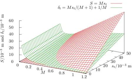
Equations 5 and 6 present the sensitivity and uncer-tainty of a BOS optical setup, respectively. Their plot as a function of the optical magnificationMand the distancest between the imaged background and the flow field is given in figure 3. This plot presents the experiment design space for unit values of f#and∆t. In practical implementations,
f#=5.6−40, and∆t=3−4×`px ≈10−20µm.
2.2 Image evaluation
The result of image recording are two images,IrandIm, i. e. reference and measurement images as vectors of grayscale values. In the image evaluation step it is required to ex-tract∆i j, which is achieved by correlation. In cross-correlation, a subset of one of the images (representing the interrogation windowW) is defined, and then its grayscale values are compared for similarity to grayscale values of all equal subsets of the other image. In this case, the vectors are multiplied and the most similar subsets yield the high-est product (maximal value being 1). The product, known
-15 -10 -5 0 5 10 15
-1200 -1000 -800 -600 -400 -200 0 200 400 600 Doa
/
10
−
3
m
Dpp/ 10−3m
st
so si
T
B L I
∆t
δb
δt
Fig. 2.Circle of least confusion∆t and spatial resolutionδtper
pixel.δbis the smallest feature on the background that can be
re-solved in imaging, effectively determining the diameter of a dot. In axes,Dppis the distance from the principal plane (the lens) and
Doais the distance from the optical axis.
S=M st δt=M st/(M+ 1) + 1/M
0 0.2
0.4 0.6
0.8 1
1.2
M 0 10
20 30 40 50
st/10−3m
0 10 20 30 40 50 60
S
/10
−
3
m
and
δt
/10
−
3m
Fig. 3.Surface plot of the sensitivityS (red surface, equation 5) and uncertaintyδt (green surface, equation 6) of a BOS system
for unit values of f# (f-number of the lens) and∆px (linear
di-mension of the pixel size). For small magnifications, uncertainty plays the determining role in adjusting the system, while for large magnifications, the system can be made quite sensitive.
as the cross-correlation coefficient, is
c(p,q)=X h
X
v
W(h, v)[Ir(h, v)− hIri]×
×W(h+p, v+q)[Im(h+p, v+q)− hImi], (7)
where hIri and hImi are the average values of reference and measurement images over windowW, andhandvare the horizontal and vertical pixel locations. The summation is done over all pixel count values, with the largest num-ber equal to the pixel count of the cameraNpx = H×V. p andq are trial displacement components. Thus, the re-sult of the cross-correlation is a spatial displacement vec-torc(p,q), which relates the correlation peaks. Applying a three point Gaussian peak detection scheme, this vector can be determined with an accuracy better than 0.1 pixel (in some implementations, down to 0.01 pixel). The mag-nitude ofc(p,q) is the amount of pixel shift due to light ray deflection of a background pattern projected (imaged) in the image plane,∆i j.
smoothen-ing from non uniform image blur, etc. Some of these ef-fects are studied by numerical experiments in synthetic im-ages, in particular the effect of the IW, the background dot size, dot density, and the introduction of blur. Half of a 128×128 pixels synthetically generated reference image of randomly distributed dots is shifted for a number of pix-els, giving the simulated measurement image. This corre-sponds to the treatment of the image with the step function H[N], where
H[N]= (
0 forN <0,
1 forN ≥0, (8)
withN =H/2. In other words, the image is sliced in two equal parts, with the right side (pixels in horizontal loca-tions 64 and higher) slided for one or more pixels to the left. Then, the simulated reference and measurement im-ages are cross-correlated. The effects are observed by the changes on the step function response width (SFWR), as defined in [35].
Image evaluation with different IW shows that the smaller the IW the closer the evaluated jump is to the real step function, as shown in figure 4. In this investigation, the simulated images had a dot the size of a pixel, and the im-age coverim-age by dots was 50%. The spread and gradual increase of the discontinuity means that there can not be an independent shift vector within the length it takes the evaluated pixel shift value to jump. Therefore, the evalu-ated spatial resolution for IW=32 pixel is about 38 pixel, and for IW=8 it is about 16 pixels. Multipass evaluation with successively smaller IW did not show any improve-ment in the evaluation of the jump, while it gave erroneous (fluctuating) values for the amount of the pixel shift.
The preparation of the background involves determina-tion of the dot size, frequency (in terms of the number of dots in the field of view), and coverage. While in experi-ments with natural backgrounds the experimenter has no control over the background features, in experiments un-der laboratory conditions (e. g. shock tube or wind tunnel experiments), the experimenter can prepare a background that optimizes the measurement based on the camera specifics and the field of view. Figure 5 shows the effect of the dot size in the resolution, where dot sizesδbequal to one and four pixels are compared after images are treated by a one pixel step function. The evaluation does not show any large effect on the resolution, but it does give different values for the pixel shift. For the case withδb=4 pixels, the effective shift of the image corresponds to a quarter of a dot, hence some pixels are not recorded as shifted. This situation ap-pears in synthetic image evaluations, because these images have a well defined binary structure. In experiments, an image of a binary background results in a grayscale im-age with spread histogram peaks around the binary values. This leads to more accurate results during evaluation. Fig-ure 6 shows the effect of dot density, which is defined as the number of dots per unit area of the field of view projected in the total image area. Maximal dot density, 50%, means that half of the image is covered by dots, and the mini-mal density simulated (5% coverage with dots) is mainly a white featureless background. As previously, the image is treated to a one pixel shift and evaluated with IW=8 pixel. Virtually, there is no difference in evaluating images with dot density of higher than 20 – 25%, but pixel shift evalu-ation artifacts start showing for images with lower number
0 0.2 0.4 0.6 0.8 1
-20 -10 0 10 20 30 40
∆
H
/
pixel
Dps/ pixel
IW(32) IW(32, 16, 8) SFRW for IW(32)
SFRW for IW(8)
H[N]
IW(8)
IW(16)
Fig. 4.The effect of the size of the interrogation window on the cross-correlation evaluation.Dpsis the distance from the location
of pixel shift,H[N] is the step function, SFRW is the step func-tion response width, and IW(a) is the interrogation window, with
abeing its value in pixels. For IW(32, 16, 8), multipass evaluation was carried out.
0 0.2 0.4 0.6 0.8 1
-20 -10 0 10 20 30 40
∆H
/
pixel
Dps/ pixel
δb= 1 pixel
δb= 4 pixels
Fig. 5.The effect of the background dot size on evaluating pixel shift.
of dots. This result is in agreement with the previously pub-lished requirement that an IW should have at least four to five dots, each covering 2 pixels.
The effect of the blur is investigated by treating the syn-thetic measurement image with a Gaussian blur of radius of 2 pixels, and the result is shown in figure 7. In this case, the image was shifted for five pixels and the interrogation window was 16 pixels. The effect of the blurring in SFRW is negligible, but this is not so for the determination of the amount of pixel shift. The blurring of the image has the ef-fect of reducing this value for about 10% and introducing fluctuations in its behaviour, thus yielding a lower signal-to-noise (S/N) ratio. This effect comes about because, as compared to the binary image, the blurred image is popu-lated by all possible grayscale values and pattern’s spatial frequency is not conserved.
3 Experiments
0 0.2 0.4 0.6 0.8 1
-20 -10 0 10 20 30 40
∆
H
/
pixel
Dps/ pixel 50% 25% 5%
Fig. 6.The effect of the dot distribution density on evaluating pixel shift.
-1 0 1 2 3 4 5 6
-20 -10 0 10 20 30 40
∆
H
/
pixel
Dps/ pixel SFRW
Binary Blurred
20 60 100 20
60 100 20 60 100
Fig. 7.Pixel shift evaluation by cross-correlation (IW=16 pixels) of binary (inset, up) and Gaussian blurred (inset, down) synthetic images with dots of one pixel, shifted for 5 pixels. Tics in insets are image pixels. Again, SFRW is virtually the same for both cases, but the S/N changes for the worst in the case of blurred images.
3.1 Shock reflection
A BOS experiment for the investigation of shock diff rac-tion and reflecrac-tion from a wedge (inclined plane) in a shock tube was conduced, with the aim of testing BOS capabili-ties, because the passage of a planar shock wave is a well studied and documented phenomenon, thus it can serve as a benchmark test. The shock tube was run with air at P1 =0.10 MPa as the driven gas and nitrogen N2atP4 = 0.35 MPa as the driver gas. The model was a stainless steel wedge with the base attached to the top of the shock tube, effectively creating an inclined plane with inclination of 49◦. Shock propagation was monitored by three Kistler 603B pressure transducers, which also sent the triggering signal for the image recording system. Timing of the exper-iment was controlled by a combination of an oscilloscope and a pulsed delay generator. Shock Mach number for all experiments was 1.3, and since the effective field of view was 220 mm×150 mm, a high speed camera was needed for freezing shock’s motion. For this reason, two types of cameras were used:
– Shimadzu HPV-1 camera with 312×260 pixel count and time resolution of 0.5µs, capable of taking 100 im-ages with a maximal frame rate of 1 Mfps. The camera
sensor is of the IS-CCD type, with a linear dimension of pixel’s light collecting area of about 50µm;
– Imacon DRS 200 camera with 1200×980 pixel count and linear dimension of pixel size approximately 6.5
µm. This camera has 7 channels, each being capable of taking two images with the fastest interframe of 1
µs, thus resulting in a total of 14 images. Since all 7 channels are independent, their respective interframes can be adjusted freely. The minimal exposure time of the camera is 5 ns, which is faster than the required and used 1µs time resolution.
The main differences between these two cameras come from their pixel count, with Imacon having a 10×better characteristic, and the pixel area, with the Shimadzu one having a 10×larger area. The background used in the shock tube experiments was a white sheet with randomly dis-tributed square dots of 1 mm side length. This background was illuminated by a xenon flashlamp that has pulse dura-tion longer than 1 ms. Although in both experiments the background was a binary image, that is with only white and black areas, the recorded image was an 8 bit grayscale digital file.
3.2 Natural convection
The steady temperature field was achieved by a cylindri-cal radiative heater with diameter of 10 mm, length of 150 mm (corresponding to w in figure 1), and power of 100 W, placed perpendicularly to the background. Since the temperature field changed slowly with time, the require-ments on the temporal resolution were minimal, so a stan-dard DSLR Pentax K-5 (digital single-lens reflex) camera was used. This camera has a sensor of 23.6 mm ×15.8 mm and pixel count of 4928×3264 pixels, hence a linear pixel size of about 5µm. The objective lens had a focal length of 300 mm and experiments were done with aper-ture of f/32. Small apertures were used in order to obtain longer depths of field. Illumination was achieved by back-lighting the printed background with a xenon flashlamp, and the camera exposure times were 1/180 s. Several types of backgrounds were generated by printing a random dot pattern in an A4 paper. Setup distances were adjusted to achieve an optical magnification of the system M = 0.1, with 30 pixels imaging 1 mm of the field of view. The tem-perature was simultaneously monitored by 2 thermocou-ples with temperature resolution of 0.1◦C.
4 Results
4.1 Instrumentation - image quality
exposure time is not a limiting factor, because it can be large enough to reach an average value of temperature read-ing smaller than the measurement uncertainty, but still be orders of magnitude smaller than the temperature measure-ment steps. Thus, one would be free to choose a camera with a high pixel count or a large sensor size, so that the image detail is satisfactory for precise measurements.
Images shown in figure 8 are from both types of high speed cameras and show a detail of the same background imaged through the test section of a shock tube. If one con-siders the sensitivity of a BOS setup based on the geome-try of the layout and the size of the image sensor, Ima-con camera would be preferable to Shimadzu, for two rea-sons: larger pixel count and smaller pixel size. But, despite the facts that the shown field of view is the same and that the images were taken with the same lens as well as un-der the same illumination, obtained images are quite dif-ferent, which fundamentally comes about due to the diff er-ent quantum efficiencies of the respective image sensors. A dramatic outcome of this difference is that the direct (without any processing) evaluation with cross-correlation of images captured by Imacon camera could not give any meaningful results, while images captured by Shimadzu did, as illustrated later. The difference can be explained through different response to luminance of the image sen-sors and the contrast values of the output file. Both cameras have a sensor with 10 bit dynamic range and give compa-rable dark images, but the histogram of the measurement images, shows that the Shimadzu camera produces a better contrast.
Since the images in BOS are of randomly scattered dots, that is structureless distribution of black and white dots, it is of prime importance that cameras yield high im-age quality. One way of determining the quality of imim-ages is by measuring the universal image quality index, as pro-posed in [36], which in a modified form is
Qmod=QLQC=
2hxihyi
hxi2hyi2 2σxσy
σ2 x+σ2y
, (9)
where xis the captured image, y is an ideal to which x is being measured, hxi andhyi are their respective aver-age values, andσx andσy their standard deviations. The first term in equation 9, QL, corresponds to the compar-ison of the luminance between images, the second term, QC, describes the comparison of the contrast between the images. The closer the imagexis to an idealy, the closer these values will be to 1. Overall,Qmod quantifies the re-sponse of the camera sensor and its quantum efficiency in a simple manner, giving a value that allows for a judgement whether a camera can give a file that can be evaluated by cross-correlation. Values ofQmodfor the cameras used in these experiments are given in table 1.
4.2 Shock reflection
Results of cross-correlation for the shock reflection exper-iment are shown in figure 9, where the magnitude map of dot displacement vector shift is plotted. The interrogation window for this evaluation was 8 pixels, thus giving a res-olution of 10 pixels. Since the optical magnification was 0.1, the measurement uncertainty then is 5 mm. As already stated when the role of the interrogation window was dis-cussed, its large value results in the spill of the pixel shifts
Fig. 8. Images on the left and on the center - the latter being the framed part of the former, - are taken with Imacon DSR200 camera, and that on the right with Shimadzu HPV-1. The left and right images show the same field of view, while the one on the center and that on the right have the same pixel count.
0 50 100 150 200 250 300 Horizontal pixel location 0
50 100 150 200 250
V
ertical
pixel
lo
cation
0 0.1 0.2 0.3 0.4 0.5 0.6 0.7 0.8
1
Fig. 9.Background oriented schlieren result for the shck reflec-tion from a wedge (black full lines), shown as a magnitude map of vector shift, with pixel locations in coordinates and pixel shift amount in the magnitude bar. The small rectangle starting at pixel (50,0) is the part of the image given in figure 8.
inside the wedge. Nevertheless, some clear features of the phenomena are observed, such as the shock wave, its re-flection, and the sonic domain.
4.3 Natural convection
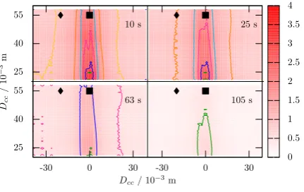
-30 0 30 -30 0 30 Dcc/ 10−3m
25 40 55 25 40 55
Dcc
/
10
−
3m
0 0.5 1 1.5 2 2.5 3 3.5 4
10 s 25 s
63 s 105 s
1
Fig. 10.BOS results for cooling by natural convection, taken at four different times: 10 s, 25 s, 63 s, and 105 s after the heater was turned off(times noted in the upper right courner of each map).Dccis the distance from the center of the heating cylinder.
Thermocouple positions are noted by the symbolsand. Co-ordinates give the distance from the center of the heat source, in mm, and the magnitude bar gives the pixel shift. Contour lines correspond to borders between zones with pixel shift diference of 0.5 pixel.
20 40 60 80 100 120 140
0 50 100 150 200 250 300 350 400 450 500
T
/
◦C
t/ s NLC
TC BOS BOS
Fig. 11.Quantitative BOS result for cooling by natural convec-tion, and the comparison of BOS data to thermocouple (TC) read-ings and Newton’s law of cooling (NLC). Here, temperatureTis given as a function of timet.
Table 1.Luminance and contrast image quality indices for high speed cameras (Imacon, Shimadzu) and standard DSLR cameras (Pentax K-5).
QL QC
Imacon DSR200 0.18 0.07 Shimadzu HPV-1 0.62 0.54 Pentax K-5 0.99 0.71
5 Prospects for ballistic range experiments
In applying the BOS technique for ballistic range measure-ments, one should take into consideration the small size of the model and its fast velocity. Current research predicts that the optimal cruise flight will be with Mach number about 1.7. The small size of the model would allow for a relatively large magnification: for a 50 mm model, and considering double the size of the field of view,M ≈0.3.
But, this would require a very fast shutter speed. During the exposure time of 1µs, a model flying at speed≈600 m·s−1will traverse more that 0.5 mm, limiting the field of view imaged by a pixel in at least 1 mm (or, alternatively, limiting the minimal size of the background dot at least at 1 mm, for a dot per pixel). As a consequence, the field of view would appear quite coarse.
An alternative is the use of short light pulse for imaging (e.g. nanosecond white light flash system, or a pulsed laser with destroyed coherence) in combination with a high res-olution camera. Increased magnification would allow for sensitive measurements, as well as for the decrease of the distance between the background and the test section, st, which would make possible having the entire test section in focus by using large depths of field.
Another improvement in spatial resolution of the mea-surement would be using single-pixel correlation, although this would require a large number of experimental images under the same conditions.
6 Conclusions
The development of background oriented schlieren (BOS) technique is advanced by assessing several factors that in-fluence the extraction of quantitative data, be it in the ex-perimental or image evaluation stage. The sensitivity and uncertainty of a BOS setup was obtained, as well as the im-age quality index was introduced to assess the instrumenta-tion. This assessment would not only assist with the judg-ment of the image quality and whether the image would yield meaningful results after cross-correlation, but also would be beneficial for diagnostics of the faulty arrange-ments (illumination or contrast).
Investigation of the geometrical arrangement of the in-struments used for BOS visualization reveal that arbitrary sensitivity and resolution can be achieved, but, these spec-ifications, though, are later deteriorated by image evalua-tion. Uncertainties related to the point of measurement are influenced by the interrogation window, defining the spa-tial resolution of the measurement, while image blurring influences the determination of the pixel shift.
In accordance to previous studies, investigation of back-ground featurres showed that a good cross-correlation eval-uation requires at least four to five dots for an interrogation window, with a dot covering two pixels.
BOS technique was applied to two types of flows, with variable success. Shock reflection from a wedge was visu-alized, albeit only qualitatively. Several features were ob-served, such as the reflected shock, and probably the acous-tic region behind the refelection. In the case of natural con-vection, the results had a quantitative nature, comparable to the results obtained with thermocouples.
Acknowledgment
This work was supported by Global Center of Excellence Program ”World Center of Education and Research for Trans-disciplinary Flow Dynamics,” Tohoku University, Japan.
References
1. H. W. Liepmann and A. Roshko,Elements of Gasdy-namics(John Wiley and Sons, New York 1957)
2. D. Igra and E. Arad, Shock Waves16, 269–273 (2007) 3. R. Hu, A. Jameson and Q. Wang, AIAA paper 2011–
1248, (2011)
4. K. Kusunose, K. Matsushima, S. Obayashi, T. Fu-rukawa, N. Kuratani,Y. Goto, D. Maruyama, H. Ya-mashita and M. Yonezawa,Aerodynamic Design of Su-personic Biplane: Cutting Edge and Related Topics – The 21st Century COE Program, International COE of Flow Dynamics Lecture Series, volume 5(Tohoku Uni-versity Press, Sendai 2007)
5. K. Kusunose, K. Matsushima and D. Maruyama, Progress in Aerospace Sciences47, 53–87 (2011) 6. N. Kuratani, T. Ogawa, H. Yamashita, M Yonezawa and
S. Obayashi, AIAA paper 2007–3674, (2007)
7. K. Saito, H. Nagai, T. Ogawa and K. Asai, Proc. of 22nd ICIASF, 1–8 (2007)
8. N. Kuratani, M. Yonezawa, H. Yamashita, S. Ozaki, T. Ogawa and S. Obayashi, Proc. of 26th ICAS, 2008-2.4ST (2008)
9. H. Kawazoe, S. Abe, T. Matsuno, G. Yamada and S. Obayashi, Proc. of 27th ICAS, 2010-2.10ST2 (2010) 10. M. Kashitani, Y. Yamaguchi, Y. Kai, K. Hirata and K.
Kusunose, AIAA paper 2008–349, (2008)
11. H. Nagai, S. Oyama, T. Ogawa, N. Kuratani and K. Asai, Proc. 26th ICAS, 2008-3.7.5 (2008)
12. A. Toyoda, M. Okubo, S. Obayashi, K. Shimizu, A. Matsuda and A. Sasoh, AIAA paper 2010–873, (2010) 13. W. Merzkirch, Flow Visualization(Academic Press,
New York, 1987)
14. W. Merzkirch, inSpringer Handbook of Experimental Fluid Mechanics, editors C. Tropea, A. L. Yarin and J. F. Foss, (Springer, Berlin 2007)
15. D. A. Forsyth and J. Ponce,Computer Vision: a Mod-ern Apporach, (Prentice Hall, New York 2002)
16. B. J¨ahne,Digital Image Processing, (Springer, Berlin 2002)
17. H. Richard and M. Raffel, Meas. Sci. Technol. 12, 1576–1585 (2001)
18. G. E. A. Meier, Exp. Fluids33, 181–187 (2002) 19. E. Goldhahn and J. Seume, Exp. Fluids43, 241–249
(2007)
20. M. Sj¨odahl, Appl. Opt.36, 2875–2885 (1997) 21. M. Raffel, C. E. Willert, S. T. Wereley and J.
Kom-penhans, Particle Image Velocimetry, (Springer, Berlin 2007)
22. F. Klinge, T. Kirmse and J. Kompenhans, Proc. of PSFVIP-4, F4097 (2003)
23. L. Venkatakrishnan and G. E. A. Meier, Exp. Fluids
37, 237–247 (2004)
24. D. Ramanah, S. Raghunath, D. J. Mee, T. R¨osgen and P. A. Jacobs, Shock Waves17, 65–70 (2007)
25. T. Mizukaki, Shock Waves20, 531–537 (2010)
26. M. Ota, K. Hamada, H. Kato and K. Maeno, Meas. Sci Technol.22, 104011 (2011)
27. M. Raffel, H. Richard and G. E. A. Meier, Exp. Fluids
28, 477–481 (2000)
28. O. K. Sommersel, D. Bjerketvedt, S. O. Christensen, O. Krest and K. Vaagsaether, Shock Waves18, 291–297 (2008)
29. M. J. Hargather and G. S. Settles, Exp. Fluids48, 59– 68 (2010)
30. K. Kindler, E. Goldhahn, F. Leopold and M. Raffel, Exp. Fluids43, 233–240 (2007)
31. B. Atcheson, W. Heidrich and I. Ihrke, Exp. Fluids46, 467–476 (2009)
32. L. Venkatakrishnan and P. Suriyanarayanan, Exp. Flu-ids47, 463–473 (2009)
33. F. Sourgen, F. Leopold and D. Klatt, Opt. Laser Eng.
50, 29–38 (2012)
34. M. Born and E. Wolf,Principles of Optics(Cambridge University Press, Cambridge 1999)
35. C. J. K¨ahler, S. Scharnowski and C. Cierpka, Exp. Flu-ids52, 1629–1639 (2012)