OIL PRICE, EXCHANGE RATE AND DISAGGREGATE CONSUMER PRICES: CAUSALITY, IMPULSE RESPONSE, AND VARIANCE DECOMPOSITION

(1)

United Kingdom Vol. V, Issue 6, June 2017

Licensed under Creative Common Page 37

http://ijecm.co.uk/

ISSN 2348 0386

OIL PRICE, EXCHANGE RATE AND DISAGGREGATE

CONSUMER PRICES: CAUSALITY, IMPULSE

RESPONSE, AND VARIANCE DECOMPOSITION

Umar Bala

Department of Economics, Faculty of Economics and Management, Universiti Putra Malaysia Department of Economics, Faculty of Management and Social Sciences,

Bauchi State University, Gadau, Nigeria [email protected]

Lee Chin

Department of Economics, Faculty of Economics and Management, Universiti Putra Malaysia [email protected]

Abstract

This study attempts to examine whether the unpredictability causes of higher prices is

connected with the changes in oil price and exchange rate. Since there are numerous consumer

prices with are affected differently by the changes in oil price and exchange rate. The study

used aggregate inflation and the disaggregated prices components annual data within the

sample period of 1976-2015. Augmented Dickey-Fuller (ADF) and Philips-Perron (PP) test were

used to neutralize data and to free them from unit-root. The Johansen Juselius (JJ)

Cointegration test was used to check if there is the prospect of long-run relation among the

variables in the models. Then from the property of VAR model the models are express in VECM

approach to ascertain the direction of a causal relationship both in the short-run and the

long-run, generalized impulse response functions (IRFs) and Variance Decomposition. The results

revealed that the causality between oil price, exchange rate are indirect related to inflation

mostly through the money supply.

Keywords: oil price, exchange rate, disaggregate consumer price, causality, impulse response,

(2)

Licensed under Creative Common Page 38 INTRODUCTION

The causes of inflation and the how a country are affected by the changes in oil prices and exchange become a major concern among policymakers. Most of the oil exporting countries are affected when oil price changes in the world market due to the nature of its fluctuation. The changes in oil price may cause the exchange rate to adjust defending whether oil price increase or decrease. Ordinarily, increases in oil price may lead to appreciation in the exchange rate in oil exporting countries while a decrease is the other way round. The adjustment of exchange rate may affect the general price especially a country which is highly depended on import. There is a lot of empirical studies on how exchange rate pass-through to inflation (Garcia 2001;Ghosh and Rajan 2009;Kara and Öğünç 2009;Jimborean 2013;Jiang and Kim 2013;Peón and Brindis

2014;Mirdala 2014). Some studies focus on the oil price pass-through to inflation (Hooker 2002; Gregorio et al. 2007; Chen 2009; Jongwanich and Park 2011; Ibrahim and Said 2012; Baumeister and Kilian 2014; Nazarian and Amiri 2014; Sakashita and Yoshizaki 2016; Hasanov et al. 2017). A country has a specific inflation target to maintain example single digit inflation in Nigeria. The country is able to maintain it a target when oil price increases as exchange rate appreciated. But it seems that when oil price decrease exchange rate depreciated inflation exceeded the central bank target. Essential the policy makers are concentrated on the general inflation targeting overlook the aggregate prices from various consumer prices which may have a different effect. Although, there are several interesting motivations that make the studies of energy prices and international finance interested especially through how oil price and exchange rate pass-through to inflation. Particularly to investigate the causal relationship between oil price, exchange rate, and inflation. Most of the studies of exchange rate pass-through are tried to look at the direct impact on economic performance, other studies on fluctuations of the exchange rate in international finance.

(3)

open economy. Find that asymmetry is mostly visible after exogenous shocks and reject the hypothesis of an asymmetric reaction of prices in a high- and the low- inflation environment. Exchange rate shocks are transmitted into aggregate inflation at a much faster rate in emerging economies than in industrials economies (Choudhri, et al., 2005; Devereux and Yetman, 2002). Doğan, (2013) also found similar results in his study using Turkish time series data ranging from

2001:10 to 2011:3 of average nominal Turkish lira (TL) against the U.S. dollar, and the manufacturing industry producer price index (MPI). The pass-through is affected positively by the aggregate demand conditions. In particular, when the economy is growing, exchange rate changes are transmitted to prices to a larger extent than otherwise. María-Dolores, (2009) studies eleven NMSs in (Bulgaria, Cyprus, the Czech Republic, Estonia, Hungary, Latvia, Lithuania, Poland, Romania, Slovakia, Slovenia and Turkey) used data from January 2000 to July 2007 applying vector autoregressive (VAR) model. Exchange rate pass-through is larger for these developing countries. Find the evidence of a larger response in energy than in manufacturing.

(4)

tended to revert to headline, which suggests that higher commodity prices have generally not produced strong effects on inflation.

RESEARCH METHODOLOGY

Econometric Method

In Standard Granger Causality (SGC) according to Granger's (1969) method, a variable Bis caused by a variable Aif Bcan be predicted better from past values of both Band Athan from past values of Balone. For a simple bivariate model, we can test if Ais Granger-causing Bby estimating Equation (1) and then test the null hypothesis in Equation (2) by using the standard Wald test.

𝐴 =∝ + 𝛾11𝑗𝑌𝑡−𝑗 + 𝛾12𝑗𝐵𝑡−𝑗 + 𝜌

𝑗 =1 𝜌

𝑗 =1

𝜇𝑡 (1)

𝐻𝑜: 𝛾12𝑗 = 0 for j=1…..,p

𝐻1: 𝛾12𝑗 ≠ 0 for at least one j

(2)

Where: ∝is a constant and𝜇𝑡is a white noise process. The variable Bis said to Granger-cause variable Aif we reject the null hypothesis (2), where 𝛾12 is the vector of the coefficients of the lagged values of the variable A. Similarly, we can test if B causes A by replacing B for A and vice versa in Equation (1). Let use the following vector autoregressive model of order 𝑃

𝐴𝑡 = ∝ +𝑋1𝐴𝑡− 1+. . . +𝑋𝑃−1𝐴𝑡−𝑃+ 𝜀𝑡 (3)

Where: 𝐴𝑡represent the cointegration variables in 5× 1 vector

𝐴1= Disaggregate consumer prices

𝐴2= Oil price

𝐴3= Exchange rate

𝐴4= GDP

𝐴5= money supply

(5)

Granger representation theorems hold if they are moving in the same direction toward the long-run equilibrium, the VAR model can be express as the following VECM model:

∆𝐴𝑡 = ∝ + 𝛤1𝑋𝑡−1+. . . +𝛤𝑃−1 ∆𝐴𝑡−𝑃+1+ 𝛱𝐴𝑡−1 + 𝜀𝑡 (4)

Where ∆ represent changes in operator, while 𝜀𝑡 represent white noise residual of the vector. When 𝛱is assumed to be cointegrated between 1 <r < 5, and it can be decompressed like this 𝛱 = 𝛼𝛽, where 𝛼(5𝑥𝑦) 𝑎𝑛𝑑 𝛽(5𝑥𝑦), also the second equation will be re expressed in this foam:

∆𝐴𝑡 = ∝ + 𝛤1𝐴𝑡−1+. . . +𝛤𝑃−1 ∆𝐴𝑡−𝑃+1+ 𝛼(𝛽′𝐴𝑡−1) + 𝜀𝑡 (5)

Where the 𝛽 rowsremain the interpreted as different cointegration vectors, also the α’s stand for the adjustment of coefficient showing the possible movement to the equilibrium in the long-run, and also linear combinations of 𝛽′𝑋𝑡−1are stationary procedures then each of the variable in Equation three is in stationary foam. The cointegration methods of Johansen (1988) allowed to check also detects the possible amount of cointegrated equation among the non-stationary variables in technique through the procedure of a maximum likelihood.

Vector Error-correction Model (VECM) Causality Tests

The Granger causality is employed to examine the short-run and long-run causality relationship among the variables in the models are: aggregate consumer price (CPI), food prices (FP), tobacco price (TA), accommodation price (AP), household price (HP), transport price (TP), other prices (O), oil price (OP), exchange rate (EX), GDP, and money supply (M2) the models are made in accordance with the VECM (Pesaran et al. 1999). Considering the following technique of vector error-correction model (VECM) model, from the long-run equation will transform in as follows:

∆𝑃 ∗1𝑡= 𝑢1+ 𝛼1,𝑕,𝐸𝐶𝑇𝑕.𝑡−𝐼 𝑟

𝑕=1

+ 𝐵11.𝑘 ∆𝑃 ∗5𝑡−𝑘 𝑝−1

𝑘=1

+ 𝐵12,𝑘 ∆𝑂𝑃1𝑡−𝑘 𝑝−1

𝑘=1

+ 𝐵13.𝑘 ∆𝐸𝑋4𝑡−𝑘 𝑝−1

𝑘=1

+ 𝐵14.𝑘 ∆𝐺𝐷𝑃5𝑡−𝑘 𝑝−1

𝑘=1

+ 𝐵15,𝑘 ∆𝑀25𝑡−𝑘 𝑝−1

𝑘=1

(6)

∆𝑂𝑃2𝑡 = 𝑢2+ 𝛼2,𝑕,𝐸𝐶𝑇𝑕.𝑡−𝐼+ 𝑟

𝑕=1

𝐵21,𝑘 ∆𝑂𝑃1𝑡−𝑘 𝑝−1

𝑘=1

+ 𝐵22,𝑘 ∆𝐸𝑋2𝑡−𝑘 𝑝−1

𝑘=1

+ 𝐵23,𝑘 ∆𝐺𝐷𝑃3𝑡−𝑘 𝑝−1

𝑘=1

+ 𝐵24.𝑘 ∆𝑀24𝑡−𝑘 𝑝−1

𝑘=1

+ 𝐵25,𝑘 ∆𝑃 ∗5𝑡−𝑘 𝑝−1

𝑘=1

+ ℰ2𝑡

∆𝐸𝑋3𝑡 = 𝑢3+ 𝛼3,𝑕,𝐸𝐶𝑇𝑕.𝑡−𝐼+ 𝑟

𝑕=1

𝐵31,𝑘 ∆𝐸𝑋1𝑡−𝑘 𝑝−1

𝑘=1

+ 𝐵33,𝑘 ∆𝑀23𝑡−𝑘 𝑝−1

𝑘=1

+ 𝐵34.𝑘 ∆𝑃 ∗4𝑡−𝑘 𝑝−1

𝑘=1

+ 𝐵35,𝑘 ∆𝑂𝑃5𝑡−𝑘 𝑝−1

𝑘=1

+ ℰ3𝑡

∆𝐺𝐷𝑃4𝑡 = 𝑢4+ 𝛼4,𝑕,𝐸𝐶𝑇𝑕.𝑡−𝐼+ 𝑟

𝑕=1

𝐵41,𝑘 ∆𝐺𝐷𝑃1𝑡−𝑘 𝑝−1

𝑘=1

+ 𝐵42,𝑘 ∆𝑀22𝑡−𝑘 𝑝−1

𝑘=1

+ 𝐵43,𝑘 ∆𝑃 ∗3𝑡−𝑘 𝑝−1

𝑘=1

+ 𝐵44.𝑘 ∆𝑂𝑃4𝑡−𝑘 𝑝−1

𝑘=1

+ 𝐵45,𝑘 ∆𝐸𝑋5𝑡−𝑘 𝑝−1

𝑘=1

+ ℰ3𝑡

∆𝑀24𝑡 = 𝑢4+ 𝛼5,𝑕,𝐸𝐶𝑇𝑕.𝑡−𝐼+ 𝑟

𝑕=1

𝐵51,𝑘 ∆𝑀21𝑡−𝑘 𝑝−1

𝑘=1

+ 𝐵52,𝑘 ∆𝑃 ∗2𝑡−𝑘 𝑝−1

𝑘=1

+ 𝐵53,𝑘 ∆𝑂𝑃3𝑡−𝑘 𝑝−1

𝑘=1

+ 𝐵54.𝑘 ∆𝐸𝑋4𝑡−𝑘 𝑝−1

𝑘=1

+ ℰ3𝑡

Where the ECTh,t−1 represent 𝑕𝑡𝑕 the error correction term the residuals from the 𝑕𝑡𝑕of one

lagged period of the cointegration equation, and 𝛽𝑖𝑗 ,𝑘 explains the effect of the 𝑘𝑡𝑕 amount of lag

in the variable 𝑗on the present amount of variable. Moreover, by generating the causal direction between the variables, VECM methodology differentiates the causality in two different ways (short-run causality and long-run causality). The above settings in the six equations, is a Granger causality in the long-run from variable 𝑌𝑖to variable 𝑋𝑗in the presence of cointegration is

estimated to examination the null hypothesis is 𝛼𝑗 ,𝑕 = 0 for 𝑕 = 1, . . . , 𝑟, however, the causality

in the short-run from variable 𝑌𝑖to variable 𝑋𝑗is estimated to examination the null hypothesis is

𝛽𝑖𝑗 ,1 = 𝛽𝑖𝑗 ,p−1 = 0,by estimating the standard F-statistic. To accept or reject between the two

null hypotheses, in accomplishing the variable 𝑌𝑖Granger causes 𝑋𝑗variable.

The Data

(7)

revenue and expenditure pushed inflation rate to 23 percent between 1975 and 1976. The variables consist eight indicators of disaggregated consumer price indexes namely aggregate consumer price (CPI), food prices (FP), tobacco price (TA), accommodation price (AP), household price (HP), clothing price (CP), transport price (TP) and other prices (O). The official exchange rate was used as a proxy for the exchange rate (EX), the Nigerian oil price Bonny Light is used as a proxy oil price, GDP per capita constants US dollar is used as economic growth, money, and quasi-money (M2) as a percentage of GDP is used as a proxy money supply. The data are extracted from the Central Bank of Nigeria (CBN) Statistical bulletin and World Bank online database and converted into natural log format.

RESULTS AND DISCUSSION

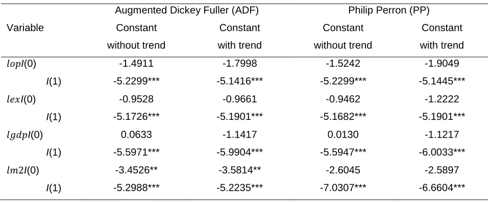
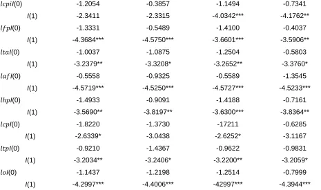
The Unit root test table below displays the outcome of the variables. The study used two most common tests in the time series literatureknown as Augmented Dickey-Fuller (ADF) and Phillips-Perron (PP) test. Based on their level or I(0), the result indicates that the null hypothesis has failed to reject or non-stationary both constant with and without trend. It is because all variables are not statistically significant at 1, 5, or at least 10 percent. Though the first differences or I(1), the result showed that all the variables at 1, 5 and 10 percent level are statistically significant. The test has processed the results of all the variables are stationary in first differences. Those variables are Log oil price, log of exchange rate, log of GDP, log of money supply, log of aggregate CPI, log of food prices, log of tobacco prices, log of accommodation price, log of household price, log of cloth price, log of transport price and log of other prices.

Table 1. Unit-root Test

Variable

Augmented Dickey Fuller (ADF) Philip Perron (PP)

Constant

without trend

Constant

with trend

Constant

without trend

Constant

with trend

𝑙𝑜𝑝I(0)

I(1)

-1.4911

-5.2299***

-1.7998

-5.1416***

-1.5242

-5.2299***

-1.9049

-5.1445***

𝑙𝑒𝑥I(0)

I(1)

-0.9528

-5.1726***

-0.9661

-5.1901***

-0.9462

-5.1682***

-1.2222

-5.1901***

𝑙𝑔𝑑𝑝I(0)

I(1)

0.0633

-5.5971***

-1.1417

-5.9904***

0.0130

-5.5947***

-1.1217

-6.0033***

𝑙𝑚2I(0)

I(1)

-3.4526**

-5.2988***

-3.5814**

-5.2235***

-2.6045

-7.0307***

-2.5897

(8)

𝑙𝑐𝑝𝑖I(0)

I(1) -1.2054 -2.3411 -0.3857 -2.3315 -1.1494 -4.0342*** -0.7341 -4.1762**

𝑙𝑓𝑝I(0)

I(1) -1.3331 -4.3684*** -0.5489 -4.5750*** -1.4100 -3.6601*** -0.4037 -3.5906**

𝑙𝑡𝑎I(0)

I(1) -1.0037 -3.2379** -1.0875 -3.3208* -1.2504 -3.2652** -0.5803 -3.3760*

𝑙𝑎𝑓I(0)

I(1) -0.5558 -4.5719*** -0.9325 -4.5250*** -0.5589 -4.5727*** -1.3545 -4.5233***

𝑙𝑕𝑝I(0)

I(1) -1.4933 -3.5690** -0.9091 -3.8197** -1.4188 -3.6300*** -0.7161 -3.8364**

𝑙𝑐𝑝I(0)

I(1) -1.8220 -2.6339* -1.3730 -3.0438 -17211 -2.6252* -0.6285 -3.1167

𝑙𝑡𝑝I(0)

I(1) -0.9210 -3.2034** -1.4367 -3.2406* -0.9622 -3.2200** -0.9831 -3.2059*

𝑙𝑜I(0)

I(1) -1.1437 -4.2997*** -1.2198 -4.4006*** -1.2514 -42997*** -0.7999 -4.3944***

Note: SIC is used to select the optimum lag order in ADF and PP test and ***, ** and * denote significance level at 1 percent, 5 percent, and 10 percent.

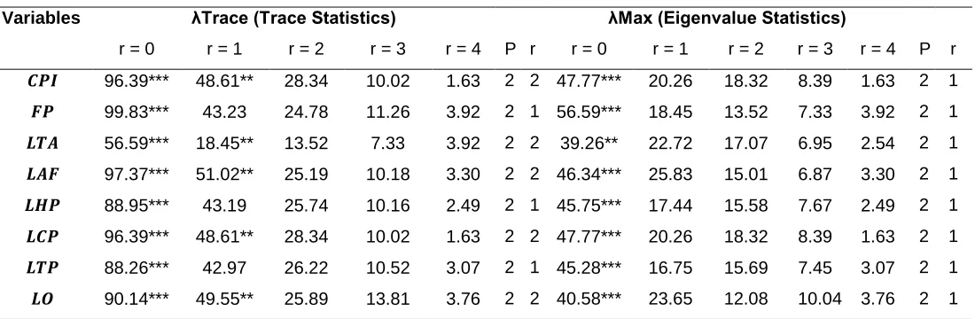
The next step is to determine the cointegration relationship between the oil price, exchange rate and the eight disaggregate consumer prices models. The Johansen cointegration test was used throughout the estimation of the long-run equations. The estimation consists two major statistics trace statistics (λtrace) and maximum eigenvalue statistics (λmax). The Johansen procedure

was chosen because has the properties to detect more than one cointegrating relationship in the long-run model rather than the Philips Ouliaris method which can detect only one cointegration relationship in the models (Ssekuma, 2011). The results obtained from the Johansen cointegration test from the two statistics Trace statistics and Max-Eigen statistics are closely similar, usually, the results may show little dissimilarities when the sample size is small(Lutkepohl and NeiSunajev 2014).The study used Akaike Information criteria (AIC) in determining the optimum lags selection in the VAR model. Table 2 provides the cointegration of eight disaggregated consumer price models indicated the evidence of long-run relations. Model 1 with aggregate consumer price trace statistics indicated 2 cointegrated vectors and eigenvalue indicated 1 vector. Model 2 with food price trace statistics indicated 1 cointegration vectors and eigenvalue indicated 1 vector. Model 3 with tobacco price indicated the existence of 2 cointegration vectors and eigenvalue indicated 1 vector. Model 4 with accommodation price indicated the existence of 2 cointegration vectors and eigenvalue indicated 1 vector. Model 5

(9)

with household price indicated the existence of 1 cointegration vector and eigenvalue indicated 1 vector. Model 6 with cloth price indicated the existence of 2 cointegration vectors and eigenvalue indicated 1 vector. Model 7 with transport price indicated the existence of 1 cointegration vector and eigenvalue indicated 1 vector. Model 8 with other prices indicated the existence of 2 cointegration vectors and eigenvalue indicated 1 vector. All the models are chosen 2 lags has optimal lags as indicated in the table, the cointegration vectors are significance at 1 percent and 5 percent level.

Table 2. Cointegration Results Based on Trace and Eigenvalue Statistics

Variables λTrace (Trace Statistics) λMax (Eigenvalue Statistics)

r = 0 r = 1 r = 2 r = 3 r = 4 P r r = 0 r = 1 r = 2 r = 3 r = 4 P r

𝑪𝑷𝑰 96.39*** 48.61** 28.34 10.02 1.63 2 2 47.77*** 20.26 18.32 8.39 1.63 2 1

𝑭𝑷 99.83*** 43.23 24.78 11.26 3.92 2 1 56.59*** 18.45 13.52 7.33 3.92 2 1

𝑳𝑻𝑨 56.59*** 18.45** 13.52 7.33 3.92 2 2 39.26** 22.72 17.07 6.95 2.54 2 1

𝑳𝑨𝑭 97.37*** 51.02** 25.19 10.18 3.30 2 2 46.34*** 25.83 15.01 6.87 3.30 2 1

𝑳𝑯𝑷 88.95*** 43.19 25.74 10.16 2.49 2 1 45.75*** 17.44 15.58 7.67 2.49 2 1

𝑳𝑪𝑷 96.39*** 48.61** 28.34 10.02 1.63 2 2 47.77*** 20.26 18.32 8.39 1.63 2 1

𝑳𝑻𝑷 88.26*** 42.97 26.22 10.52 3.07 2 1 45.28*** 16.75 15.69 7.45 3.07 2 1

𝑳𝑶 90.14*** 49.55** 25.89 13.81 3.76 2 2 40.58*** 23.65 12.08 10.04 3.76 2 1

Note: *** and **: indicate significance at 1% and 5%, levels.

λtrace is the trace statistics value and .λmax is the maximum eigenvalue statistics. P indicates

the optimal lag length based on AIC from the unrestricted VAR model. r is the number of cointegration vectors based on Johansen’s method.

The confirmation the mutual relationship in the long-run has satisfied the requirement to testify the direction of Granger causality between oil price, exchange rate, and inflation. Since, when the variables are cointegrated, there must be a possibility of the existence of Granger causality of a minimum of one-way direction(Granger, 1988). Since the existence of cointegration does not an indication the direction of causal relationship among them. The only provide the evidence of the existence of Granger causality. The possible way to detect the causal relationship is to use the vector error correction model (VECM) which originated directly from the cointegration vectors.

(10)

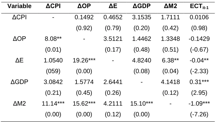
clarified the possibility of causality effects in two categories: the short-run and the long-run. The second column is for t-test while the third column is for F-test and both of them are to determine the either the null hypothesis is accepted or rejected. Therefore to avoid the spurious regression results problem, the model as a feature of error correction term to capture the variations related to the adjustment level in long-run. The study further estimated the VECM base causality tests by applying Johansen cointegration vectors. The direction of causality between the variables in the model with the aggregate CPI which indicate that in the short-run CPI is causes oil price, oil price causes oil price-exchange rate, money supply cause exchange rate, CPI cause money supply, oil price cause money supply, GDP cause money supply. While in the long-run exchange rate and money supply models are significant meanings that cause CPI in the long-run. The results reveal that in the short-run the impact of exchange rate on aggregate CPI is indirect through the other indicators in the model.

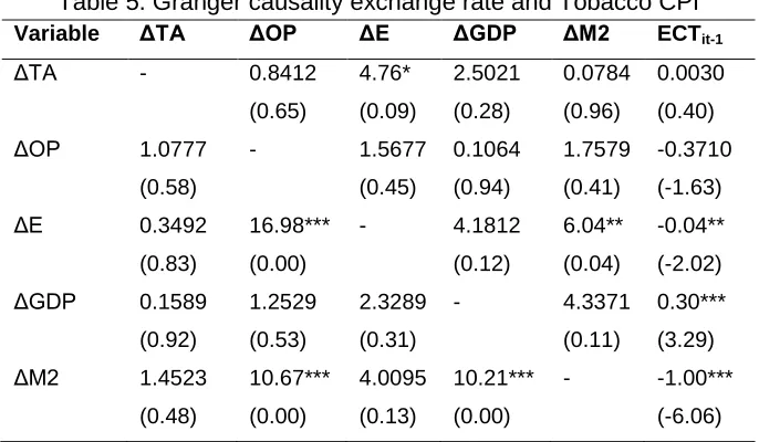
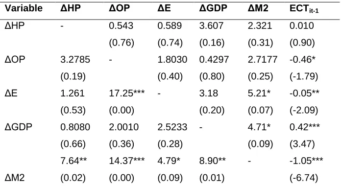
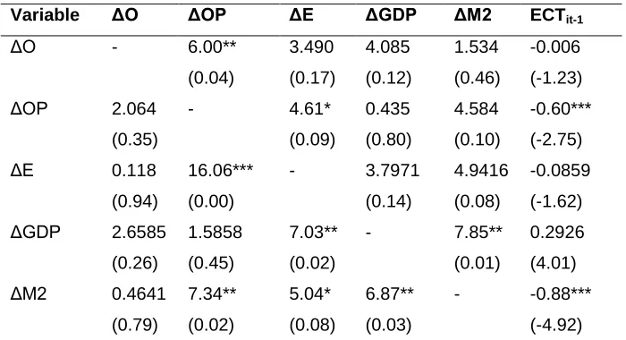
Table 4 to 10 presents the direction of causality with the disaggregated CPI. Table 4 present the result indicate that in the short-run oil price is causes exchange rate, food price, oil price, exchange rate and GDP are causes oil money supply. Whereas in the long-run model indicate that exchange rate and money supply is significant meanings that cause prices in the long-run. The results reveal that in the short-run the impact of exchange rate on aggregate CPI is indirect through the oil price and money supply. The other disaggregate prices has different long-run causality as indicate in the models.

Table 3. Granger causality exchange rate Aggregate CPI

Variable ΔCPI ΔOP ΔE ΔGDP ΔM2 ECTit-1

ΔCPI - 0.1492

(0.92)

0.4652

(0.79)

3.1535

(0.20)

1.7111

(0.42)

0.0106

(0.98)

ΔOP 8.08**

(0.01)

- 3.5121

(0.17)

1.4462

(0.48)

1.3348

(0.51)

-0.1429

(-0.67)

ΔE 1.0540

(059)

19.26***

(0.00)

- 4.8240

(0.08)

6.38**

(0.04)

-0.04**

(-2.33)

ΔGDP 3.0842

(0.21)

1.5774

(0.45)

2.6441

(0.26)

- 4.1418

(0.12)

0.31***

(2.95)

ΔM2 11.14***

(0.00)

15.62***

(0.00)

4.2111

(0.12)

15.10***

(0.00)

- -1.09***

(11)

Table 4. Granger causality exchange rate and Food CPI

Variable ΔFP ΔOP ΔE ΔGDP ΔM2 ECTit-1

ΔFP - 0.8224

(0.66) 3.0864 (0.21) 0.6623 (0.71) 2.0638 (0.35) -0.0127 (-0.43)

ΔOP 0.8651

(0.64)

- 2.0553

(0.35) 0.2678 (0.87) 0.5169 (0.77) -0.2685 (-1.03)

ΔE 0.9358

(0.62)

15.40***

(0.00)

- 2.8375

(0.24)

3.6160

(0.16)

0.0252

(1.83)

ΔGDP 2.3929

(0.30)

1.0986

(0.57)

1.2319

(0.54)

- 1.4681

(0.47)

0.3436

(3.00)

ΔM2 6.45**

(0.03) 11.74*** (0.00) 6.05** (0.04) 9.57*** (0.00)

- -1.00***

(-6.00)

Table 5. Granger causality exchange rate and Tobacco CPI

Variable ΔTA ΔOP ΔE ΔGDP ΔM2 ECTit-1

ΔTA - 0.8412

(0.65) 4.76* (0.09) 2.5021 (0.28) 0.0784 (0.96) 0.0030 (0.40)

ΔOP 1.0777

(0.58)

- 1.5677

(0.45) 0.1064 (0.94) 1.7579 (0.41) -0.3710 (-1.63)

ΔE 0.3492

(0.83)

16.98***

(0.00)

- 4.1812

(0.12)

6.04**

(0.04)

-0.04**

(-2.02)

ΔGDP 0.1589

(0.92)

1.2529

(0.53)

2.3289

(0.31)

- 4.3371

(0.11)

0.30***

(3.29)

ΔM2 1.4523

(0.48) 10.67*** (0.00) 4.0095 (0.13) 10.21*** (0.00)

- -1.00***

(-6.06)

Table 6. Granger causality exchange rate and Accommodation CPI

Variable ΔAF ΔOP ΔE ΔGDP ΔM2 ECTit-1

ΔAF - 0.338

(0.84) 1.618 (0.44) 0.507 (0.77) 0.150 (0.92) 0.008 (0.52)

ΔOP 3.714

(0.15)

- 3.897

(0.14) 0.709 (0.70) 1.779 (0.41) -0.35* (-1.82)

ΔE 1.7119

(0.42)

19.75***

(0.00)

- 5.44*

(0.06)

8.10**

(0.01)

0.29***

(3.07)

ΔGDP 4.64*

(0.09)

1.1276

(0.56)

3.6699

(0.15)

- 2.9704

(0.22)

-0.12**

(-2.27)

ΔM2 14.67***

(0.00) 8.38** (0.01) 4.3852 (0.12) 8.94** (0.01)

- -0.82***

(12)

Table 7. Granger causality exchange rate and Household CPI

Variable ΔHP ΔOP ΔE ΔGDP ΔM2 ECTit-1

ΔHP - 0.543

(0.76) 0.589 (0.74) 3.607 (0.16) 2.321 (0.31) 0.010 (0.90)

ΔOP 3.2785

(0.19)

- 1.8030

(0.40) 0.4297 (0.80) 2.7177 (0.25) -0.46* (-1.79)

ΔE 1.261

(0.53)

17.25***

(0.00)

- 3.18

(0.20)

5.21*

(0.07)

-0.05**

(-2.09)

ΔGDP 0.8080

(0.66)

2.0010

(0.36)

2.5233

(0.28)

- 4.71*

(0.09) 0.42*** (3.47) ΔM2 7.64** (0.02) 14.37*** (0.00) 4.79* (0.09) 8.90** (0.01)

- -1.05***

(-6.74)

Table 8. Granger causality exchange rate and Clothing CPI

Variable ΔCP ΔOP ΔE ΔGDP ΔM2 ECTit-1

ΔCP - 0.149

(0.92) 0.465 (0.79) 3.153 (0.20) 1.711 (0.42) 0.010 (0.98)

ΔOP 8.08**

(0.01)

- 3.5121

(0.17) 1.4462 (0.48) 1.3348 (0.51) -0.1429 (-0.67)

ΔE 1.0540

(0.59)

19.26***

(0.00)

- 4.82*

(0.08)

6.38**

(0.04)

-0.04**

(-2.33)

ΔGDP 3.0842

(0.21)

1.5774

(0.45)

2.6441

(0.26)

- 4.1418

(0.12)

0.31***

(2.95)

ΔM2 11.14***

(0.00) 15.62*** (0.00) 4.211 (0.12) 15.10*** (0.00)

- -1.09***

(-7.26)

Table 9. Granger causality exchange rate and Transport CPI

Variable ΔTP ΔOP ΔE ΔGDP ΔM2 ECTit-1

ΔTP - 0.257

(0.87) 2.494 (0.28) 4.337 (0.11) 1.122 (0.57) 8.21 (0.01)

ΔOP 2.5288

(0.28)

- 1.8707

(0.39) 0.3476 (0.84) 0.5515 (0.75) -0.27 (-1.24)

ΔE 1.7884

(0.40)

20.06***

(0.00)

- 4.0033

(0.13)

6.53**

(0.03)

-0.06**

(2.21)

ΔGDP 4.85*

(0.08)

1.421

(0.49)

2.563

(0.27)

- 2.723

(0.25)

0.32***

(3.32)

ΔM2 10.32***

(13)

Table 10. Granger causality exchange rate and Others CPI

Variable ΔO ΔOP ΔE ΔGDP ΔM2 ECTit-1

ΔO - 6.00**

(0.04)

3.490

(0.17)

4.085

(0.12)

1.534

(0.46)

-0.006

(-1.23)

ΔOP 2.064

(0.35)

- 4.61*

(0.09)

0.435

(0.80)

4.584

(0.10)

-0.60***

(-2.75)

ΔE 0.118

(0.94)

16.06***

(0.00)

- 3.7971

(0.14)

4.9416

(0.08)

-0.0859

(-1.62)

ΔGDP 2.6585

(0.26)

1.5858

(0.45)

7.03**

(0.02)

- 7.85**

(0.01)

0.2926

(4.01)

ΔM2 0.4641

(0.79)

7.34**

(0.02)

5.04*

(0.08)

6.87**

(0.03)

- -0.88***

(-4.92)

Note: ECTit-1 is the error correction term indicating the long-run causality

*, **, *** shows the significance levels at the 10%, 5%, and 1%, respectively.

(14)

Licensed under Creative Common Page 50 CONCLUSIONS AND POLICY IMPLICATIONS

The study examines the causality, impulse response and variance decomposition of oil price and exchange rate on disaggregated consumer prices in Nigeria. The study used aggregate inflation and the disaggregated prices components annual data within the sample period of 1976-2015. Augmented Dickey-Fuller (ADF) and Philips-Perron (PP) test were used to neutralize data and to free them from unit-root. The Johansen Juselius (JJ) Cointegration test was used to check if there is the prospect of long-run relation among the variables in the models. Then from the property of VAR model the models are express in VECM approach to ascertain the direction of a causal relationship both in the short-run and the long-run, generalized impulse response functions (IRFs) and Variance Decomposition. The study concludes that the causality between oil price, exchange rate are indirect related to inflation mostly through the money supply. The results highlight the policymakers on numerous aspects that need additional care Firstly, the confirmation of indirect causality of oil price, exchange rate are giving the insight to use contractionary monetary policy to reduce the amount of money in circulation. Furthermore, in the disaggregated consumer prices, there is different causality direction that the policy makers need to consider during the policy formation to reduce inflation. The impact of oil price and exchange rate pass-through to inflation results has implications first for economic modeling based on disaggregate and for policymakers to target specific price among the consumer prices that will reduce the high level of inflation. For further research, it is recommended to explore the nonlinear impact of oil price and exchange rate changes on inflation.

REFERENCES

Baumeister, C., & Kilian, L. (2014). Do oil price increases cause higher food prices? Economic Policy, 29(80), 691–747. http://doi.org/10.1111/1468-0327.12039

Brahmasrene, T., Huang, J. C., & Sissoko, Y. (2014). Crude oil prices and exchange rates: Causality,

variance decomposition and impulse response. Energy Economics, 44, 407–412.

http://doi.org/10.1016/j.eneco.2014.05.011

Calvo, G. A., & Reinhart, C. M. (2000). Fear of floating. National Bureau of Economic Research, (No. w7993).

Campa, J. M., & Goldberg, L. S. (2002). Exchange rate pass-through into import prices: A macro or micro phenomenon? National Bureau of Economic Research, (No. w8934).

Cecchetti, S. G., & Moessner, R. (2008). Commodity prices and inflation dynamics. BIS Quarterly Review. Retrieved from http://ideas.repec.org/a/bis/bisqtr/0812f.html

Chang, J.-C., & Tsong, C.-C. (2010). Exchange rate pass-through and monetary policy: A

cross-commodity analysis. Emerging Markets Finance and Trade, 46(6), 106–120.

http://doi.org/10.2753/REE1540-496X460607

(15)

Licensed under Creative Common Page 51 Choudhri, E. U., Faruqee, H., & Hakura, D. S. (2005). Explaining the exchange rate pass-through in

different prices. Journal of International Economics, 65, 349–374.

http://doi.org/10.1016/j.jinteco.2004.02.004

Choudhri, E. U., & Hakura, D. S. (2006). Exchange rate pass-through to domestic prices: Does the inflationary environment matter? Journal of International Money and Finance, 25(4), 614–639. http://doi.org/10.1016/j.jimonfin.2005.11.009

De Gregorio, J., Landerretche, O., & Neilson, C. (2007). Another pass-through bites the dust? Oil prices and inflation. Economía, 7(2), 155–196. http://doi.org/10.1353/eco.2007.0014

Devereux, M. B., & Yetman, J. (2002). Menu costs and the long-rub output-inflation trade-off. Economics Letters, 76(1), 95–100. http://doi.org/10.1016/S0165-1765(02)00022-8

Doğan, B. Ş. (2013). Asymmetric behavior of the exchange rate pass-through to manufacturing prices in Turkey. Emerging Markets Finance and Trade, 49(3), 35–47. http://doi.org/10.2753/REE1540-496X490303

Doroodian, K., & Boyd, R. (2003). The linkage between oil price shocks and economic growth with inflation in the presence of technological advances: a CGE model. Energy Policy, 31(10), 989–1006. http://doi.org/10.1016/S0301-4215(02)00141-6

Doyle, E. (2004). Exchange rate pass-through in a small open economy: the Anglo-Irish case. Applied Economics, 36(5), 443–455. http://doi.org/10.1080/00036840410001682142

Garcia, R. (2001). Price inflation and exchange rate pass-through in Chile. Central Bank of Chile Working Papers, (128).

Ghosh, A., & Rajan, R. S. (2009). Exchange rate pass-through in Korea and Thailand: Trends and determinants. Japan and the World Economy, 21(1), 55–70. http://doi.org/10.1016/j.japwor.2008.01.002

Goldfajn, I., & Werlang, S. R. D. C. (2000). The pass-through from depreciation to inflation: a panel study. Banco Central de Brasil Working Paper, (5).

Granger, C. W. (1988). Some recent development in a concept of causality. Journal of Econometrics, 39(11–2), 199–211.

Guillermo Peón, S. B., & Rodríguez Brindis, M. A. (2014). Analyzing the exchange rate pass-through in Mexico: Evidence post inflation targeting implementation. Ensayos Sobre Política Económica, 32(74), 18– 35. http://doi.org/10.1016/S0120-4483(14)70025-9

H. Ibrahim, M., & Said, R. (2012). Disaggregated consumer prices and oil price pass-through: evidence

from Malaysia. China Agricultural Economic Review, 4(4), 514–529.

http://doi.org/10.1108/17561371211284858

Hasanov, F., Mikayilov, J., Bulut, C., & Suleymanov, E. (2017). The role of oil prices in exchange rate movements: The CIS oil exporters. Economies, 5(2), 1–18. http://doi.org/10.3390/economies5020013

Hooker, M. a. (2002). Are oil shocks inflationary? Asymmetric and nonlinear specifications versus

changes in regime. Journal of Money, Credit and Banking, 34(2), 540–561.

http://doi.org/10.1353/mcb.2002.0041

Ibrahim, M. H. (2015). Oil and food prices in Malaysia: A nonlinear ARDL analysis. Springer Open Journal, 3(2), 1–14. http://doi.org/10.1186/s40100-014-0020-3

Ibrahim, M. H., & Chancharoenchai, K. (2014). How inflationary are oil price hikes? A disaggregated look at Thailand using symmetric and asymmetric cointegration models. Journal of the Asia Pacific Economy, 19(3), 409–422. http://doi.org/10.1080/13547860.2013.820470

Jiang, J., & Kim, D. (2013). Exchange rate pass-through to inflation in China. Economic Modelling, 33, 900–912. http://doi.org/10.1016/j.econmod.2013.05.021

(16)

Licensed under Creative Common Page 52 Jongwanich, J., & Park, D. (2011). Inflation in developing Asia: Pass-through from global food and oil price shocks. Asian-Pacific Economic Literature, 25(1), 79–92. http://doi.org/10.1111/j.1467-8411.2011.01275.x

Kara, H., & Öğünç, F. (2009). Inflation targeting and exchange rate pass-through: The Turkish experience. Emerging Markets Finance and Trade, 44(6), 52–66. http://doi.org/10.2753/REE1540-496X440604

Koop, G., Pesaran, M. H., & Potter, S. M. (1996). Impulse response analysis in nonlinear multivariate models. Journal of Econometrics, 74(1), 119–147.

Lutkepohl, H., & NeiSunajev, A. (2014). Disentangling demand and supply shocks in the crude oil market: How to check sign restrictions in structural VARs. Journal of Applied Econometrics, 29(3), 479–496.

María-Dolores, R. (2009). Exchange rate pass-through in Central and East European countries. Eastern European Economics, 47(4), 42–61. http://doi.org/10.2753/EEE0012-8775470403

McCarthy, J. (1999). Pass-Through of exchange rates and import prices to domestic inflation in some industrialized Countries. Federal Reserve Bank of New York.

Mirdala, R. (2014). Exchange rate pass-through to consumer prices in the European transition economies. Procedia Economics and Finance, 12(March), 428–436. http://doi.org/10.1016/S2212-5671(14)00364-5

Nazarian, R., & Amiri, A. (2014). Asymmetry of the oil price Pass-through to inflation in Iran. International Journal of Energy Economics and Policy, 4(3), 457–464.

Pesaran, M. H., & Shin, Y. (1998). Generalized impulse response analysis in linear multivariate models. Economics Letters, 58(1), 17–29. http://doi.org/10.1016/S0165-1765(97)00214-0

Przystupa, J., & Wróbel, E. (2011). Asymmetry of the exchange rate pass-through. Eastern European Economics, 49(1), 30–51. http://doi.org/10.2753/EEE0012-8775490103

Sakashita, Y., & Yoshizaki, Y. (2016). The effects of oil price shocks on IIP and CPI in emerging countries. Economies, 4(20), 1–9. http://doi.org/10.3390/economies4040020

(17)

Licensed under Creative Common Page 53 APPENDICES

.00 .02 .04 .06 .08 .10 .12

1 2 3 4 5 6 7 8 9 10

Res pons e of LCPI to Choles ky One S.D. LE Innovation

-.100 -.075 -.050 -.025 .000 .025 .050

1 2 3 4 5 6 7 8 9 10

Res pons e of LOP to Choles ky One S.D. LE Innovation

-.24 -.20 -.16 -.12 -.08 -.04

1 2 3 4 5 6 7 8 9 10

Res pons e of LGDP to Choles ky One S.D. LE Innovation

-.06 -.04 -.02 .00 .02 .04

1 2 3 4 5 6 7 8 9 10

Res pons e of LM2 to Choles ky One S.D. LE Innovation

0 20 40 60 80 100

1 2 3 4 5 6 7 8 9 10

LCPI LOP LE LGDP LM2

(18)

-.04 .00 .04 .08 .12 .16

1 2 3 4 5 6 7 8 9 10

Res pons e of LFP to Choles ky One S.D. LE Innovation

-.100 -.075 -.050 -.025 .000 .025 .050

1 2 3 4 5 6 7 8 9 10

-.24 -.20 -.16 -.12 -.08 -.04

1 2 3 4 5 6 7 8 9 10

-.06 -.04 -.02 .00 .02 .04

1 2 3 4 5 6 7 8 9 10

0 20 40 60 80 100

1 2 3 4 5 6 7 8 9 10

LFP LOP LE LGDP LM2

(19)

.00 .04 .08 .12

1 2 3 4 5 6 7 8 9 10

Res pons e of LTA to LE

-.100 -.075 -.050 -.025 .000 .025 .050

1 2 3 4 5 6 7 8 9 10

Res pons e of LOP to LE

-.16 -.14 -.12 -.10 -.08 -.06 -.04

1 2 3 4 5 6 7 8 9 10

Res pons e of LGDP to LE

-.04 -.03 -.02 -.01 .00 .01 .02

1 2 3 4 5 6 7 8 9 10

Res pons e of LM2 to LE

Response to Cholesky One S.D. Innovations

0 20 40 60 80 100

1 2 3 4 5 6 7 8 9 10

LTA LOP LE LGDP LM2

(20)

-.01 .00 .01 .02 .03 .04

1 2 3 4 5 6 7 8 9 10

Res pons e of LAF to LE

-.04 .00 .04 .08

1 2 3 4 5 6 7 8 9 10

-.16 -.12 -.08 -.04

1 2 3 4 5 6 7 8 9 10

-.06 -.05 -.04 -.03 -.02 -.01 .00 .01

1 2 3 4 5 6 7 8 9 10

0 20 40 60 80 100

1 2 3 4 5 6 7 8 9 10

LAF LOP LE LGDP LM2

(21)

.00 .04 .08 .12 .16

1 2 3 4 5 6 7 8 9 10

Res pons e of LHP to Choles ky One S.D. LE Innovation

-.12 -.08 -.04 .00 .04

1 2 3 4 5 6 7 8 9 10

-.20 -.16 -.12 -.08 -.04

1 2 3 4 5 6 7 8 9 10

-.04 -.03 -.02 -.01 .00 .01 .02 .03

1 2 3 4 5 6 7 8 9 10

0 20 40 60 80 100

1 2 3 4 5 6 7 8 9 10

LHP LOP LE LGDP M2

(22)

.00 .02 .04 .06 .08 .10 .12

1 2 3 4 5 6 7 8 9 10

Res pons e of LCP to LE

-.100 -.075 -.050 -.025 .000 .025 .050

1 2 3 4 5 6 7 8 9 10

-.24 -.20 -.16 -.12 -.08 -.04

1 2 3 4 5 6 7 8 9 10

-.06 -.04 -.02 .00 .02 .04

1 2 3 4 5 6 7 8 9 10

0 20 40 60 80 100

1 2 3 4 5 6 7 8 9 10

LCP LOP LE LGDP LM2

(23)

.00 .02 .04 .06 .08 .10 .12

1 2 3 4 5 6 7 8 9 10

Res pons e of LTP to LE

-.06 -.04 -.02 .00 .02 .04 .06

1 2 3 4 5 6 7 8 9 10

-.14 -.12 -.10 -.08 -.06 -.04 -.02

1 2 3 4 5 6 7 8 9 10

-.06 -.05 -.04 -.03 -.02 -.01 .00 .01

1 2 3 4 5 6 7 8 9 10

0 20 40 60 80 100

1 2 3 4 5 6 7 8 9 10

LTP LOP LE LGDP LM2