Published online July 20, 2013 (http://www.sciencepublishinggroup.com/j/ijepe) doi: 10.11648/j.ijepe.20130203.17
Mathematical modelling, finite element simulation and
experimental validation of biogas-digester slurry
temperature
Suresh Baral
1, 2, *, Shiva P. Pudasaini
3, Sanjay Nath Khanal
4, Dil Bahadur Gurung
31
School of Engineering, Pokhara University, Kaski, Nepal 2
Department of Mechanical Engineering, Kathmandu University, Kavre, Nepal 3
Department of Mathematical Sciences, Kathmandu University, Dhulikhel, Kavre, Nepal 4
Department of Environmental Science and Engineering, Kathmandu University, Dhulikhel, Kavre
Email address:
[email protected](S. Baral)To cite this article:
Suresh Baral, Shiva P. Pudasaini, Sanjay Nath Khanal, Dil Bahadur Gurung. Mathematical Modelling, Finite Element Simulation and Experimental Validation of Biogas-digester Slurry Temperature. International Journal of Energy and Power Engineering.
Vol. 2, No. 3, 2013, pp. 128-135. doi: 10.11648/j.ijepe.20130203.17
Abstract:
The present describes and simulates the temperature distribution of slurry by using the heat equation and appropriate boundary conditions and their numerical simulations with the Finite Element Method. This method is suitable to describe the temperature profile in Bio-digester and Bio-rectors for optimum biogas production. The Mathematical modeling of bio-digester helps us to understand the change in digester temperature with the change in the ambient temperature, internal heat generation, thermal conductivity and other physical and thermo-dynamical processes that govern the thermal system. Mathematical modeling can also be used to predict and estimate the physical and chemical parameters affecting the biogas production. The internal heat generation was estimated to be 1.2 W/m3.The Finite Element linear, quadratic solutions and exact solution was compared for the profile of temperature of the bio-digester slurry. The average temperature of bio-digester slurry was found to be 33.12 °C at its center. The thermal conductivity we have also found to be0.69 W/ m °C. By using the finite element method to solve the mathematical modeling, the maximum slurry temperature was found to be 33.13 °C at its center. Furthermore, we have calculated the thermal conductivity in the biogas chamber from our measurement data. This thermal conductivity (k) 0.69 W/m °C was used in the exact solution of the physical model equation, linear and quadratic finite elements solutions. The temperature profiles of these three solutions virtually collapse to a single parabolic profile, which in term agreed very well with our measured data of the temperature profile.
Keywords
:
Mathematical Modeling, Slurry Temperature, Thermal Conductivity, Biogas-Digester, Finite Element Method, Internal Heat Generation1. Introduction
Nepal, one of the least developed countries, is categorized by very low per capita energy consumption. Because of a lack of other commercial sources of energy, the country relies heavily on traditional fuel source, especially firewood. In order to solve the energy problem in rural areas, the country initiated production and distribution of several renewable energy technologies. Among several technologies, biogas has been proved to be viable and emerged as a promising technology. It has been one of the most successful models for the production of clean, environmental friendly, cost effective source of energy and
International Journal of Energy and Power Engineering 2013; 2(3): 128-135 129
considered to be reliable, well-functioning, simple, low maintenance cost and durable. Within the dome, bacteria, which occur naturally in cow dung, break down the raw materials to produce methane. Cattle manure, human excreta and agriculture residues are used in anaerobic bioreactors in many parts of the world to produce methane gas, which is used for the purpose of cooking and lighting. Since such waste materials are readily available in farms, rural people of many developing countries have been benefited from this technology. Besides, this technology is cheaper and simpler, thus, gaining popularity throughout the world. Nepal is one of the least developed countries with the vast majority of people involved in subsistence agriculture. The use of biogas technology in Nepal has benefited the country in improving health, environment, economy and energy conservation [2].The reaction in the biogas plant takes place in the absence of oxygen and the gas contains up to 70 per cent methane and 30 per cent carbon dioxide. At the top of the dome there is a gas outlet pipe that is connected to the house hold appliances. Once the gas is produced, the remaining matter comes out as slurry, which can be used as organic fertilizer.
The objectives of paper were
a) To develop a general one-dimensional model based on fundamental principle of conservation of energy to predict the temperature distribution and other important physical properties of slurry such as thermal conductivity (k), and internal heat generation (fe) by using the Ritz Finite
Element Method (FEM).The main aim is to generate experimental data of temperature in the digester and calibrate the mathematical computational model.
b) To develop a Finite Element Model for the simulation of the physical variable e.g. the temperature distribution in the biogas-digester.
c) To check the Finite Element Method model prediction against the measured data.
d) To analyze the physical and geometrical parameters of the digester and the digester process by using the Finite Element Method (FEM) so as to design the efficient digester from engineering point of view.
Production of biogas by digestion of organic wastes and other feedstock is one of the important technical solutions that contribute to the transform of the energy system from being fossil fuel dependent to renewable energy originated. To be fully commercial and competitive, the production of biogas needs to be further developed and optimized based on the technical, economic and environmental aspects. Thus, comprehensive understanding of fluid dynamics and microbial reactions in the digestion process is necessary to accurately and robustly model, predict and control the biogas production. In this paper possible pathways for modeling the biogas reactor is discussed based on previous work on anaerobic digestion modeling and modeling of the fluid flow in reactors. Important parameters for modeling biogas production, with a focus on processes using waste as feedstock, are considered. Identification of knowledge gaps for the modeling of the biogas process is performed and
how to overcome the obstacles is addressed. Biswas et al.[3]
experimented on anaerobic digester of 10 L ca
pacity
operated in batch mode at an optimum temperature of 40 °C and at a pH of 6.8 using vegetable/food residues as the feed material
for modeling of biogas digester.
Rapport et al. [4] developed a model to predict the mass and energy balance for a full-scale high-solids anaerobic digester using research data from lab and pilot scale systems and estimated the Costs, revenues project cash flow, net present worth (NPW), simple payback, internal rate of return, and revenue requirements. Li et al. [5] studied the feasibility of using synthetic kitchen waste (KW) and fat, oil, and grease (FOG) as co-substrates in the anaerobic digestion of waste activated sludge (WAS) using two series of biochemical methane potential (BMP) tests and modeled had been developed. Liliana et al. [6] concluded that the mathematical modeling is useful in determining the temperature and biogas production. The working temperature of bio-reactor was 37 °C with the thermal conductivity of 0.6197 W/m°C for biogas generation without any bacteria to die off.
2. Methods and Materials
For conducting of experiment, cattle dung slurry was prepared with the ratio of distribution of dung and water is 1:1. The digester of 1 m radius and digester volume of 4 m3 was taken as research work which was located in Kathmandu University, Dhulikhel. The total cattle dung used in digester is approximately 2500 kg. The hydraulic retention time was 25 days. The temperature was measured every day in the mid-day during hydraulic retention time. The initial temperature without pre-heating of slurry was found to be 25 °C. The anaerobic fermentation starts after the temperature difference of 2°C [7]. The temperature measurements were taken on radial distance of bio-digester in the top layer. Three equidistant points were marked on the radial distance for daily temperature measurements. The measurements were stopped once the temperatures in successive days were near steady state. The temperature measurements were carried out by using digital temperature measurement with an uncertainty ±0.05°C. Finite Element solution codes were written with commercial software Matlab 5 and the results were analyzed. For validation of the model, the temperature of slurry is observed from 10th day of feeding to final production of gas.
3. Mathematical Modeling and its Finite
Element Simulation for Heat
Transfer Problem
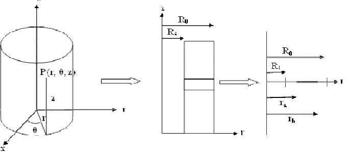
equation is a diffusion equation. The problem is known as axisymmetric when the geometry, loading and boundary conditions are independent of the circumferential dire (i.e. θ-coordinates), so this governing equation in turn
Figure 1.Volume element and computational domain of an axisymmetric problem
The governing equation of the problem is as follows
)
(
)
(
1
r
f
dr
du
r
a
dr
d
r
=
−
forR
= radial coordinateA
=k
r
(k
is the thermal conductivity) = known functions ofr
u
= temperature= dependent variablef
= internal heat generation= known functions ofi
R
= inner radius of cylindero
R
=outer radius of cylinderThe finite element model is obtained by substituting approximation
1
( ) ( ) (2)
n e e j j j
u r u
ψ
r=
≈
∑
and
w
=
ψ
1,
ψ
2,...
.
ψ
n, the finite element model is given by{ } { } {
e e e e
K u f Q
= +
Where
2 , 2
b b
a a
e
r e r
j
e i e e
ij i i
r r
d d
K a dr f f r dr
dr dr
ψ ψ
π π ψ
=
∫
=∫
And
ψ
eiis the interpolation functions expressed in terms of the radial coordinater
. The linear interpolation functions are of the form (h
e=
r
b−
r
a).1( ) , 2( )
e b e a
e e
r r r r
r r
h h
ψ = − ψ = −
equation is a diffusion equation. The problem is known as axisymmetric when the geometry, loading and boundary conditions are independent of the circumferential direction coordinates), so this governing equation in turn
converts to two-dimensional in terms of r and z. If the problem geometry and data are independent of z, the equations are functions of only the radial coordinate r
Volume element and computational domain of an axisymmetric problem
The governing equation of the problem is as follows
o
i
r
R
R
<
<
(1)is the thermal conductivity) = known
= temperature= dependent variable
= internal heat generation= known functions of
r
The finite element model is obtained by substituting
( ) e e( ) (2)
j j
u r
∑
uψ
r, the finite element model
}
(3)e e e e
K u f Q
2 , 2
b b
a a
r r
e e e
ij i i
r r
K = π
∫
a dr f = π ψ∫
f r dr (4)is the interpolation functions expressed in terms . The linear interpolation functions
1( ) , 2( )
e b e a
e e
r r r r
r r
h h
ψ = − ψ = − (5)
The quadratic interpolation functions expressed in terms of the radial coordinate r.
The forms of the coefficients
and f = fe are given below.
Linear Element
[ ]
=
π
h
a
2
K
e e{ }
e 2f =
Quadratic Element
(
(
)
(
3 14 4 16 2
4 16 16 32 12 16
2 12 16 11 14
e a e a e a
e a e a e a
e a e a e a
h r h r h r
h r h r h r
h r h r h r
+ − + + − + + − + + − + +
{ }
f
e=
2π
The following data were considered for numerical computations.
Assuming, natural convection (β) = 3 W/ Wall temperature of slurry (T
Outer radius (R0) = 1 m.
Thermal conductivity of slurry (k) = (Calculated)
Internal heat generation (fe)
dimensional in terms of r and z. If the problem geometry and data are independent of z, the equations are functions of only the radial coordinate r [8-9].
Volume element and computational domain of an axisymmetric problem
The quadratic interpolation functions expressed in terms
The forms of the coefficients
K
eij andf
ie for a = aer
−
−
+
1
1
1
1
)
h
2
1
r
(
a ee , (6) 3 2 3 2 6 a e e e a e r h f h r h
π
+ = + (7)
e K
=
2 e
e a h π
)
(
)
)
3 14 4 16 2
4 16 16 32 12 16
2 12 16 11 14
e a e a e a
e a e a e a
e a e a e a
h r h r h r
h r h r h r
h r h r h r
+ − + + − + + − + + − + + (8)
6
h
f
e eπ
+
+
e a e a ah
r
h
2
r
4
r
(9)The following data were considered for numerical
natural convection (β) = 3 W/ m2 °C Wall temperature of slurry (T0) = 32.7 °C
Thermal conductivity of slurry (k) = 0.69W/m°C
International Journal of Energy and Power Engineering 2013; 2(3): 128-135 131
It is important to note that the value of (fe) is estimated
from the Newton’s Law of Cooling. Assuming the natural convection is 3 W/m2 °C. Exact mathematical solution exists for this simple diffusion problem. This is advantageous here, because the measured temperature values at known spatial position and the estimated value of internal heat generation can be inspected in to the exact
solution as in
(
)
−
−
=
22o 2 o e
o
R
r
1
T
U
4
R
f
k
from which the conductivity is estimated. Although the determination of k by experiment could be difficult and time consuming the estimation of k by our method is very crucial as (k) is one of the key parameters for generating the Finite Element solution of the problem. Similarly, the value of (k) is estimated with this value of (fe) and from the known exact
solution for T for which T values were replaced by its measured values in the radial direction from the center to the chamber wall.
4. Results and Discussion
The temperature of digester was measured in May, 2010, Dhulikhel, Nepal (Altitude-1441 Meters, Latitude- N 270 – 36' – 992” Longitude – E 850 33' 432”). The values so obtained were the three nodal temperatures at the radial
distance of bio-digester. One at the outer wall of digester, other two are in mid- point and center of digester respectively as shown in figure 2.
Figure 2. Nodal points in Biogas Digester
Where node 1 denotes outer wall temperature of digester, node 2 denotes midpoint temperature of radius between center and wall and node 3 denotes center of digester temperature
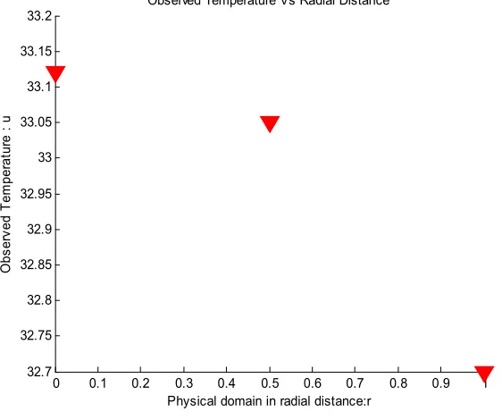
4.1. Observed Temperature Profile
Figure 3. Twelve linear elements showing temperature profile by FEM
4.2. Calculation of Thermal Conductivity of Cattle Dung (k)
The calculated value for the thermal conductivity of cattle dung (k) is 0.69 W/ m °C. This is the first step of initiation of calculation. The thermal conductivity was calculated by the boundary temperature observed during the experiment when the process became steady state. The
program code was developed for physical parameter i.e. thermal conductivity of the exact solution of the heat transfer problem in Finite Element Method by using boundary temperature. The observed temperature was plotted and the center of digester temperature was found to be 33.11 °C.
4.3. Results for the Temperature Distribution Using FEM
Y
0 0.1 0.2 0.3 0.4 0.5 0.6 0.7 0.8 0.9 1 32.7
32.75 32.8 32.85 32.9 32.95 33 33.05 33.1 33.15 33.2
Physical domain in radial distance:r
O
b
s
e
rv
e
d
T
e
m
p
e
ra
tu
re
:
u
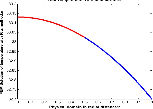
4.3.1. Twelve Linear Elements
Figure 4. Twelve linear elements showing temperature profile by FEM
This graph shows that the temperature profile of bio-digester slurry temperature with twelve linear elements by using Finite Element Method. This suggests that the center of bio-digester with its source at its vertex has temperature
33.13 °C when the wall boundary temperature is 32.7 °C.
4.3.2. Two Quadratic Elements
Figure 5. Twoquadratic elements showing temperature profile by FEM
This graph shows that the temperature profile of bio-digester slurry temperature with two quadratic elements by using Finite Element Method for obtaining more accurate
temperature. This also suggests that the center of bio-digester with its source at its vertex has temperature 33.13 °C when the wall boundary temperature is 32.7 °C.
0 0.1 0.2 0.3 0.4 0.5 0.6 0.7 0.8 0.9 1 32.7
32.75 32.8 32.85 32.9 32.95 33 33.05 33.1 33.15 33.2
Physical domain in radial distance:r
F
E
M
S
o
lu
ti
o
n
o
f
te
m
p
e
ra
tu
re
w
it
h
R
it
z
m
e
th
o
d
:u
FEM Temperature Vs Radial Distance
0 0.1 0.2 0.3 0.4 0.5 0.6 0.7 0.8 0.9 1 32.7
32.75 32.8 32.85 32.9 32.95 33 33.05 33.1 33.15 33.2
Physical domain in radial distance:r
F
E
M
S
o
lu
ti
o
n
o
f
te
m
p
e
ra
tu
re
w
it
h
R
it
z
m
e
th
o
d
:u
International Journal of Energy and Power Engineering 2013; 2(3): 128-135 133
4.3.3. Exact Solution of Heat Transfer Problem
Figure 6. Exact solution of heat transfer problem
This graph shows the temperature profile of exact solution of heat transfer problem by Finite Element Method. Here the exact solution of the heat transfer problem also suggests that the temperature at the center of digester to be 33.13 °C.
The results help in knowing how the experimented
results are correlated with the simulation method. This also helped to validate the experimented bio-gas digester slurry temperature.
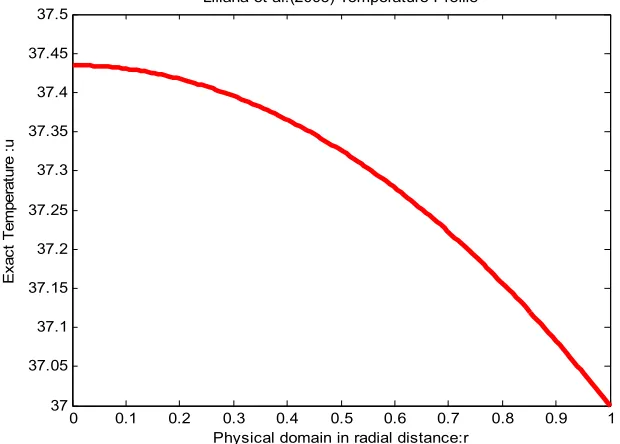
4.3.4. Temperature Simulation for Liliana et al. [6]
Figure 7. Temperature simulation for Liliana et al.[6]
This graph shows the temperature profile of Bio-reactor of radius 0.6 m, a research conducted by Liliana et al. [6]. The Bio-reactor was operated at 37 °C. The thermal
conductivity calculated for the research work was used to obtain the temperature profile of Bio-reactor. The temperature at the center of Bio-reactor was found to be
0 0.1 0.2 0.3 0.4 0.5 0.6 0.7 0.8 0.9 1
32.7 32.75 32.8 32.85 32.9 32.95 33 33.05 33.1 33.15 33.2
Physical domain in radial distance:r
E
x
a
c
t
T
e
m
p
e
ra
tu
re
:
u
Exact Temperature Vs Radial distance
0 0.1 0.2 0.3 0.4 0.5 0.6 0.7 0.8 0.9 1 37
37.05 37.1 37.15 37.2 37.25 37.3 37.35 37.4 37.45 37.5
Physical domain in radial distance:r
E
x
a
c
t
T
e
m
p
e
ra
tu
re
:
u
37.43 °C. Here the boundary temperature was assumed to be 37 °C during steady state condition.
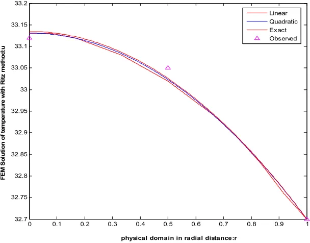
4.3.5. Graph for FE-linear, FE-quadratic and Exact Solution and Observed Data
Figure 8. FE-linear, FE-quadratic and Exact Solution, and Observed Data
This graph shows the FE-linear, FE- quadratic, Exact Solution, and observed temperature overlapping to a single line virtually, suggesting approximately the same temperature at the center of bio-digester to be 33.13 °C.
The simulation method proved that linear, quadratic and experimental data are almost similar.
5. Conclusion
The paper presented the temperature distribution in biogas digester slurry temperature by finite element method. Due to some technical difficulties, only a limited data were generated. However, still, some temperatures were measured for bench-mark problem in the field of biogas-digester. To the best of our knowledge the simulation of the bio-digester slurry temperature by the Finite Element Method (FEM) has not been carried out before, as the literature review showed. We implemented the FEM to the heat diffusion equation to simulate the temperature distribution in the digester as a pioneering work as far as the simulation tools and the physical parameter estimation methods are concerned. This heat conduction was assumed to be in the steady state. The Finite Element Method in heat transfer problem describes the heat dynamics. Since the exact solution of the heat conduction model exists, it was possible to estimate the most important parameter once the internal heat generation parameter (fe) is obtained from the
measured temperature. The free parameter, internal heat generation, was first estimated from the Newton’s Law of Cooling. The internal heat generation (fe) was found to be
1.2 W/m3 is a reasonable estimation which was later used to estimate the thermal conductivity and ultimately the entire
simulation of temperature profile. The estimated thermal conductivity (k) was found to be 0.69 W/m °C. The estimated values of the physical parameters (fe) and (k)
were then used to obtain the Finite Element simulation of temperature profile. The temperature profile was generated along the radial distance of Bio- Digester.
Furthermore, heat equation and finite elements solution was calibrated by using the measured temperature and then estimated values of (fe) and (fe) based on this measurement.
It is very important to note that, in similar physical situations, the estimated values of (fe) and (k) can be used
in future for further studies of biogas production, and also for complicated geometry. Here, we have initiated Finite element solution only for one-dimensional problem. However, this work can be extended for two and three dimension that in general may better predict the dynamics. For inhomogeneous material distribution in the bio-digester or stratification of material or any other situation in which the material properties are not constant in the problem domain, the FE simulation technique is generally the most appropriate numerical technique to describe the flow on deformation dynamics including the heat dynamics in biogas-digester/reactors.
Finally, the simulation was carried out again for the experiment conducted by Liliana et al. [6] the thermal conductivity so obtained during the research work was used for estimating the internal heat generation of bio-reactor. The internal heat generation of bio-reactor was estimated to be 12 W/ m3 where the working temperature was 37 °C and this estimation of could be a very important information to simulate the temperature distribution for the chamber.
Instead of cattle dung for biogas production, if solid
0 0.1 0.2 0.3 0.4 0.5 0.6 0.7 0.8 0.9 1
32.7 32.75 32.8 32.85 32.9 32.95 33 33.05 33.1 33.15 33.2
physical domain in radial distance:r
F
E
M
S
o
lu
ti
o
n
o
f
te
m
p
e
ra
tu
re
w
it
h
R
it
z
m
e
th
o
d
:u
International Journal of Energy and Power Engineering 2013; 2(3): 128-135 135
organic wastes are used, the production of gas is maximized [10-13]. The thermal conductivity of composite material such as solid organic waste can be calculated by the developed computer program code for bio-digester. So, solid organic waste plays greater role in reducing the energy crisis by producing huge amount of biogas in digester, which is the prime important sector in renewable energy in Nepal to be developed in today’s context.
References
[1] Katuwal, Hari, and Alok K. Bohara. "Biogas: A promising renewable technology and its impact on rural households in Nepal." Renewable and Sustainable Energy Reviews 13.9 (2009): 2668-2674.
[2] Gautam, Rajeeb, Sumit Baral, and Sunil Herat. "Biogas as a sustainable energy source in Nepal: Present status and future challenges." Renewable and Sustainable Energy Reviews 13.1 (2009): 248-252.
[3] Biswas, J., R. Chowdhury, and P. Bhattacharya. "Mathematical modeling for the prediction of biogas generation characteristics of an anaerobic digester based on food/vegetable residues." Biomass and Bioenergy 31.1 (2007): 80-86.
[4] Rapport, J. L., Zhang, R., Jenkins, B. M., Hartsough, B. R., & Tomich, T. P."Modeling the performance of the anaerobic phased solids digester system for biogas energy production." Biomass and Bioenergy35.3 (2011): 1263-1272.
[5] Li, Chenxi, Pascale Champagne, and Bruce C. Anderson. "Evaluating and modeling biogas production from municipal
fat, oil, and grease and synthetic kitchen waste in anaerobic co-digestions." Bioresource technology 102.20 (2011): 9471-9480.
[6] Zashkova, Liliana, Nina Penkova and Rositza Karamfilowa."Heat transfer processes in a biogas-reactor." Task Quarterly 9.4 (2005): 427-438.
[7] Mittal, K. M. Biogas systems: principles and applications. New Age International Limited Publishers, 1996.
[8] Rao, Singiresu S. "The finite element method in engineering." (1986).
[9] Reddy, Junuthula Narasimha. An introduction to the finite element method. Vol. 2. No. 2.2. New York: McGraw-Hill, 1993.
[10] DeWalle, Foppe B., Edward Hammerberg, and Edward SK Chian. "Gas production from solid waste in landfills." Journal of the Environmental Engineering Division 104.3 (1978): 415-432.
[11] Reinhart, Debra R., and A. Basel Al-Yousfi. "The impact of leachate recirculation on municipal solid waste landfill operating characteristics." Waste Management & Research 14.4 (1996): 337-346.
[12] Kayhanian, M., and S. Hardy. "The impact of four design parameters on the performance of a high‐solids anaerobic digestion of municipal solid waste for fuel gas production." Environmental technology 15.6 (1994): 557-567.