http://www.sciencepublishinggroup.com/j/ijssn doi: 10.11648/j.ijssn.20170503.11
Trajectory Tracking of locomotive Using IMM-Based Robust
Hybrid Control Algorithm
Tanuja Parameshwar Patgar
1, *, Shankaraiah
21
SJCE Research Center, Mysore, India 2
Department of ECE, SJCE, Mysore, India
Email address:
[email protected] (T. P. Patgar), [email protected] (Shankaraiah) *
Corresponding author
To cite this article:
Tanuja Parameshwar Patgar, Shankaraiah. Trajectory Tracking of locomotive Using IMM-Based Robust Hybrid Control Algorithm. International Journal of Sensors and Sensor Networks. Vol. 5, No. 3, 2017, pp. 34-42. doi: 10.11648/j.ijssn.20170503.11
Received: June 4, 2017; Accepted: June 26, 2017; Published: August 10, 2017
Abstract:
Locomotive surveillance is the most active research topic and still faces big technical challenges in railway safety control system. An end-to-end locomotive tracking and continuous monitoring system is necessary for safety measures in satellite visible and low satellite visible environment. These smart systems aim to updates the information on location, exact detection, speed limitation and also rail track information. This paper contributes to develop an intelligent tracking and monitoring system based on Internet of Things (IoT) platform using Differential Global Positioning System (DGPS) for improved tracking accuracy of locomotive in both environments. Interacting Multiple Model (IMM) tracking algorithm based on Di-filter model is proposed for analysis that make it easy to pinpoint the location and its status of the locomotive.Keywords:
DGPS, Di-filter, IMM Algorithm, Model Matching, Tracking Surveillance Model1. Introduction
Many real world applications managed in military and civilian require accurate tracking of moving targets acquired by sensors. In military applications, tracking is continuously updated the performance of target’s position and also tracking of enemy vehicles so that they are blocked and destroyed immediately [1]. In civilian applications target tracking is of much use in autonomous vehicles, home security etc. Accurate target tracking is used in many situations to accommodate the need for constant human help and thus it is simple to achieve much higher degree of intelligent, wireless and automatic [2]. There is loads of real time application for locomotive tracking and monitoring using satellite based navigation system with high level of speed and precision. These systems are more accurate, precise, efficient, low cost and less economic maintenance. But in poor satellite visible areas such as mountains, tunnel, valleys, deep cuttings etc. they are facing many service failure issues [3].
Land vehicle navigation technologies mainly depend on the Global Positioning System (GPS). The user platform mainly based on receiver which receives the radio signals
from four or more satellites provides the position and velocity information. In spite of diverse application of GPS, the flexibility of service is still limited as the GPS based tracking accuracy is decreases when it passes through poor satellite visible areas such as tunnel, mountain, forest, slope, bridge, urban or canopy areas due to signal failure and attenuation [4, 6]. Different locations have affected by different atmosphere factors which vary with locations and these errors are corrected by Differential GPS. The most enhanced version of Global Positioning System is Differential Global positioning System (DGPS) [8]. It provides precise and improved location tracking accuracy than GPS. It increases the tracking accuracy of the target locations or the coordinates which are derived from the GPS receivers. For improvement in tracking accuracy and monitoring the integrity of GPS satellite radio transmissions, it provides differential correction to GPS receiver. With DGPS receivers, the position tracking accuracy is improved from 30m to better than 2m.
The kinematic quantities such as position, velocity and acceleration are to be estimated. Kalman Filters are used in measurement model to reduce the errors due to noise in the observation and state process model to accurately predict the target’s estimation parameters. State estimation of potentially locomotive tracking in satellite visible and low visible often requires the use of filter models to account for varying target behavior in two different environments [14]. Efficient management of the Di-filter models for two different areas is critical to limiting algorithm computations while achieving the desired tracking performance. This requirement is achieved with the Interacting Multiple Model (IMM) algorithm. Di-filter models enable tracking system to better match changing target dynamics. In this paper, we propose Di-filter model management for the IMM algorithm that is governed by Markov chain that controls the switching behavior among the two models [15].
The organization of the paper is as follows. Section (2) explains the surveillance integration model based on Differential GPS navigation system in which how data are communicated to central office. The Di-filter model based on Kalman filter concept is proposed with Interacting Multiple Model (IMM) algorithm is depicted in section (3). Section (3.1) describes the problem formulation to track the locomotive using Di-Filter design parameters. The explanation in Section (3.2) is about the selection of tracking performance model and how it depends on the measurement noise also explains the designed target (locomotive) state kinematics models for both environment Section (4) explains the problem formulation decision logic for Di-filter and its general steps to resolve noises. Section (5) explains simulation set up using Mat Lab. The results and analysis of the moving locomotive kinematics such as position and
velocity estimation accuracy graph with related effects on noise inputs are explained. Finally section (6) depicts concluding remarks.
2. Sensor Accuracy Remote Access
Surveillance Wireless Automatic
Tracking Heuristic Innovation
(SARASWATHI) Model
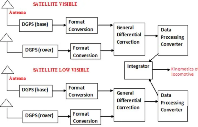
This paper highlights the main suggestion to improve the performance of locomotive detection and continuous tracking by contributing originally two different segment environments (a) satellite visible environment (b) poor satellite visible environment. Hence an accurate and efficient continuous tracking capability at the core of such system is essential for building higher level Internet of Things (IoT) vision-based intelligence system. The major objective of ground based surveillance system is to track, detect and recognize the moving object in the allocated area. For continuous tracking and monitoring of locomotive movement in satellite visible and poor satellite visible environment, a sensor based wireless surveillance model is proposed. The on-board locomotive tracking model called “Sensor Accuracy Remote Access Surveillance Wireless Automatic Tracking Heuristic Innovation (SARASWATHI)” is designed with the satellite based navigation system called Differential GPS. This model measure the position, velocity and other current state values of the locomotive when it is travels in satellite visible and low satellite visible areas. Figure. 1 describes the block diagram of surveillance heuristic model based on wireless sensor based Differential GPS technology.
Figure 1. Block diagram of remote surveillance innovation model.
Differential Global Positioning System (DGPS) is consider as one of the best accurate and precise satellite based navigation system. Its function is to identify specific location
receivers that use these measured position to compute signal timing along with increase in measurement tracking accuracy. The mobile receivers calculate the absolute positions with increased accuracy by altering their received satellite measurements in co-ordination with base station. Pre-processing is then carried out to convert the different input data from various satellites in to other prescribed readable format for Human Machine Interfacing (HMI) unit. The improved accuracy advancement offered by DGPS takes on greater significance in the 21st century. This is because the use of highly accurate positional information is collected from navigational aids like Automatic Identification system, Electronic Information and chart display system.
3. Proposed Interacting Multiple Model
(IMM) Algorithm for Di-Filter Model
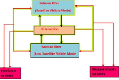
Di-filter model is designed with two tuned Kalman filter for satellite visible and satellite low visible environment model. In real-time application, tracking the locomotive in satellite visible and low satellite visible environment leads to variations in filter accuracy performance. Using Di-filter model built with two tuned Kalman filter is proposed here to track the locomotive trajectory easily. The low satellite visible tracking filter model degrades the tracking accuracy performance. Hence, we propose Interacting Multiple Model (IMM) algorithm for analysis. The filter bank is designed in such a way that one could be satellite visible filter model (X1) and the other could be based on poor
satellite visible model (X2). The IMM algorithm is one such
algorithm which combining state hypotheses from multiple filter models to get better state estimate of targets with varying dynamics [16]. The filter models used to form each state hypothesis are derived to match the behavior of targets. Figure 2 shows the flow diagram for an IMM algorithm with two filter models.
Figure 2. A block diagram of the IMM algorithm with Di-filter model.
IMM algorithm is recursive estimator having modular structure. Generally it consists of four major steps – interaction, mode-conditioned filtering, probability evaluation, combined state and covariance estimation.
3.1. Proposed Di-Filter Algorithm and Design Parameters
The state estimates for satellite visible (X1) and poor
satellite visible filter (X2) model are mixed prior to state
update using set of conditional model probabilities. The con-ditional model probabilities PIJ are computed using the model
probabilities from the previous update and state switching matrix selected a priori. The mixed state estimates are updated using each Kalman filter model. The likelihood (Aj )
for each filter model is computed during the state update from the innovations (Zi) and innovations covariance matrix [17]. The likelihood, prior model probabilities and state switching matrix are then used to update the filter model probabilities. The estimates from each Kalman filter model are combined like weighted sum using the updated model probabilities. The following steps outlined about how we are design IMM algorithm using Di-filter model.
1. Model set consisting of possible target (locomotive) tracking mode such as constant position model, constant velocity model and constant acceleration model.
2. Process noise variances for the adopted models with different regimes of target (locomotive) motion is tracked using low-level process noise covariance matrix for satellite visible model and high-level process noise for low satellite visible model.
3. Mode transition probabilities to switch from one mode to another.
The equations governing the IMM algorithm for an ‘N’ number of filter models are outlined in equation (9). The process then begins with the computed quantities from the previous filter iteration. Initialization procedures are required to obtain the state estimate, covariance, and initial probabilities for each filter model.
3.2. Proposed Design Methodology for State Kinematics Models for Both Environments
In this research work, the problem formulation is concentrate on the type of locomotive motion in satellite visible and poor satellite visible environment. The locomotive is constrained to move in straight line with constant velocity. Let X (k) is locomotive position and X’ (k) is locomotive velocity are consider fruitfully. Let V (k) be the measurement noise observed during kinematics calculation process. By consider, the locomotive is moving with constant speed X” k) = 0. The systems states consider are position, velocity and acceleration. The state parameters are [X, Y, Z] where X= Position, Y= Velocity, Z= Acceleration.
Tracking state model
Let us consider the state tracking and measurement model for locomotive position and velocity only. The tracking kinematic parameter are along X and Y co-ordinates with the time interval from n to n+1. Let us consider X (k), Y (k) are locomotive position tracking values in two direction and X1 (k), Y1 (k) are locomotive velocity tracking parameters respectively.
Where A = system transition matrix and B= process noise gain matrix
A=
1 δt δt 2 δt 3
0 1 δt δt 2
0 0 1 δt
0 0 0 1
B=
δt 3 δt
2 δt
1
∂t is a sampling interval
X (k+1) = A X (k) + B u (k)
x(k + 1) x′(k + 1) y(k + 1) y′(k + 1)
= A
x(k) x′(k) y(k) y′(k)
+ B
u (k) u ′(k)
u (k) u (k)
If the time interval is from i to i-1, then the tracking state model equation becomes
X (k) = A X (k-1) + B u (k-1) (2) A and B matrices remains same. Where E {u (k)}= 0 and Variance{u (k) } = M,
Where M = Target model noise co-variance matrix. Measurement Model
The output equation is given by
Y (k) = C X (k) + V (k) (3) Where C is sensor output
C=
1 δt δt 2 δt 3
0 1 δt δt 2
0 0 1 δt
0 0 0 1
If δt=0 C =
1 0 0 0 0 1 0 0 0 0 1 0 0 0 0 1 Y (k)
Y ′(k) Y (k) Y ′(k)
=
1 0 0 0 0 1 0 0 0 0 1 0 0 0 0 1
x(k) x′(k) y(k) y′(k)
+ v (k) v (k) v (k) v (k)
E {v (k)} = 0, Variance {v (k)} = N Where N is Measurement noise co-variance matrix.
Prediction updates
Filter predicts the state and variance at time i+1 based on information at time i. This is also known as time updates. The equations are responsible for projecting forward the current state and error covariance estimates to obtain the priori estimates for the next time step.
(1)State Prediction: X# (i + 1 i) = A X# (i i)
(2)Prediction Covariance: P&(i + 1 i) = A P& (i i) AT + M (i) Measurement updates
Kalman filter updates the state and variance using combination of the predicted state and the observation Y (i+1). These equations are responsible for the feedback which incorporates new measurement in to priori estimate to obtain an improved posteriori estimate.
(1)State estimate: X# (i + 1 i + 1 ) = X&(i + 1 i) + K [Yi
-CX# (i + 1 i) ]
(2)Estimation Covariance: P# ( i + 1 i + 1 ) = [I-KC] P#(i + 1 i)
Gain matrix
To minimize the conditional mean-squared estimation error with respect to the Kalman gain.
Kalman gain: K = P# (i + 1 i) CT [C P '(i + 1 i) CT + N]-1
3.3. Adopted Algorithm for Analysis of Kalman Filter Model
The Kalman filter is a recursive predictive filter that is based on the use of state space techniques and recursive algorithms. It is estimated the state of dynamic system. This dynamic system can be disturbed by some noise, mostly assumed as white noise. The tracking accuracy is determined by the movement of locomotive in straight line. To perform this, algorithm is build with set of nominal design parameters.
Function Value [X prediction, P prediction ] = Predict ( X, P, A,
M)
X prediction = A* X;
P prediction = A*P*A1 + M;
Function Value [Difference, T] = Dynamic ( X prediction, P prediction, Y, C, N)
Difference = Y-C* X prediction;
T = N+C * P prediction *C1
Function Value [ X KUSHI, PKUSHI] = Dynamic @ update (X prediction, P prediction, Diff, T, C)
K= P prediction *H1*T1
X KUSHI = X prediction +K*Difference
P KUSHI = P prediction – K*T*K1
Nominal Parameters used in algorithm
A). Sensor Location: S1 = [0, 0, 0] and S2 = [60, 0, 0] B)
Positional Measurement error -X direction= 0.0001 m, C). Sampling interval–1 sec D) Initial track reading - 0.8 E) Process Noise Covariance = 0.8 * Measurement error covariance F) Initial State Estimate Covariance- Position Variance = 0.1 [X, Y] Velocity Covariance = 0.0001 [X, Y]
3.4. Problem Analysis of DI-Filter Using Model Matching Technique
In this section, we presented a procedure for finding stable transfer function which in turn increase the tracking accuracy. Let us consider satellite visible model (X1) with A
(Z) is an i-th degree polynomial for stable controllable and observable transfer function. Similarly for low satellite visible model (X2) with B (Z) is an j-th degree polynomial
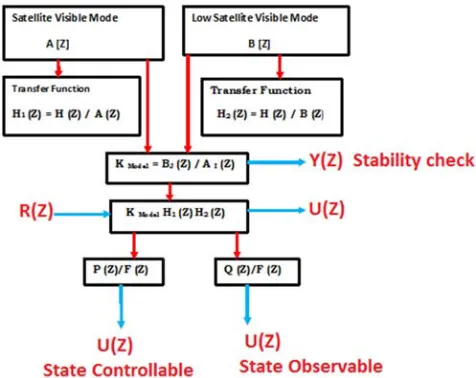
Figure 3. depicts the block diagram of model matching control system.
Figure 3. Block diagram of model matching control system.
Under certain conditions, it is possible to design such system by use of polynomial equation approach with desired stable transfer function act exactly like the model. For the closed loop system, the transfer function of the di-filter model is noted as,
Y (Z) / U (Z) = Polynomial of satellite low visible model
B (Z) / Polynomial of satellite Visible model A (Z)
Where A (Z) is an i-th degree polynomial for satellite visible model and B (Z) is an j-th degree polynomial for low satellite visible model. We assume that there is no common factor between the two models. Under certain conditions it is possible to design model system by use of the polynomial equation approach. Since we consider the transfer function of the control system exactly like the model, we call such model matching control system.
In the design process, we choose the resulting system transfer function as
H1 (Z) = H (Z) / A (Z) for satellite visible model and H2 (Z)
= H (Z) / B (Z) for satellite low visible environment.
As Y (Z) / R (Z) = K Model = BJ (Z) / A I (Z) (4)
We assume that the plant B (Z) / A (Z) is completely state controllable and completely observable function F (Z) with stable polynomial of (n-1) th degree. Using Di-ophantine equation,
P (Z) A (Z) + q (Z) B (Z) = F (Z) B (Z) H1 (Z) (5)
Where p (Z) and q (Z) are polynomial of (n-1) degrees. From the block diagram, it is analyzed the controllable and stable system resultant output as
U (Z) = - [p (Z)/F (Z)* U (Z) – U (Z) + q (Z) / F (Z) *Y (Z)] +V (Z)
P (Z)/F (Z)* U (Z) + q (Z) / F (Z) *Y (Z) = V (Z) (6) Since U (Z) = A (Z) / B (Z) * Y (Z), We have p (Z)/F (Z)* A (Z) / B (Z) * Y (Z) + q (Z) / F (Z) *Y (Z) = V (Z)
Y (Z) / V (Z) = F (Z) B (Z) / p (Z) A (Z) + q (Z) B (Z) = F (Z) B (Z) / F (Z) B (Z) H1 (Z) = 1/ H1 (Z)
V (Z) = K Model H1 (Z) R (Z), Y (Z)/ R (Z) = Y (Z) V (Z) / V (Z) R (Z) = K Model H 1 (Z) / H 1 (Z) = K Model
V (Z)/ R (Z) = K Model H1 (Z) (7)
The significance of above equation is said to be improvement in stability of the system model. First order homogeneous Markov chain,
Q{ K j (p+1) / K i(p) } = Q i (8)
¥ i, j ∑ K Where ‘K’ is a set of possible model. The model switching carried out using Markov process with known transition probabilities. The set of modes may consist of several target models.
4. Performance Analysis of Di-Filter Decision Logic
Design parameters for the Di-filter based on IMM algorithm are selected to control filter operating characteristics such as gain, measurement noise and response to operating modes such as satellite visible environment model (X1) and poor satellite
visible model (X2). The required design parameters for the filtering methods defined in the performance comparison are the
IMM state target matrix and the filter model values. Step1. The interaction of Model
The initial conditions for the filters for all ¥ i, j ∑ K
) 1 | 1 ( ) 1 | 1 ( ˆ )
1 | 1 ( ˆ
| 1
0 − − =
∑
− − − −=
k k
k k
X k
k
X i j
r
i i
(9)
Step 2 – Probability testing process
Mixing Probabilities --
Initial mode probabilities corresponding to satellite visible and poor satellite visible mode can be taken as 0.8 and 0.2 Mode transition probability
p)*= + 0.80.62 0.33/0.2 Where P12 is chosen 0.2 assuming that satellite visible model starts with a low probability. Assume
expected dwell time in a mode is 4 sec. Step-3 Mode conditioned filtering
The states and covariance estimates using the standard prediction and updates steps for each mode matched filter. The equations are
Likelihood functions for mode matched filter is given by
Step-4 Over all state and covariance estimate values
Average mode probabilities obtained are used as weighting factor to combine the updated state and covariance.
The above steps make it possible to calculate the tracking accuracy of locomotive in both satellite visible and low satellite visible environments with multiple point targets simultaneously without any a priori performance about the target (locomotive) movement.
5. Simulation Results and Discussion
We considered the state estimation problem of locomotive movement in two environments such as satellite visible and
low satellite visible environment. Simulations were executed to compare the performance of IMM algorithms with the Di-filter (Kalman) model for tracking locomotive in two different environments. Di-filter kinematic models were used to track the locomotive in two different environments with the help of constant velocity and position model and by then comparing the performance of two different model using IMM algorithm. It is assumed that the locomotive moves straight in the satellite visible area and its initial positions and velocities were differently note for each case. The
single-) 1 | 1 ( ] )} 1 | 1 ( ˆ ) 1 | 1 ( ˆ { )} 1 | 1 ( ˆ ) 1 | 1 ( ˆ [{ ) 1 | 1 ( ) 1 | 1 ( | 1 0 0
0 − −
− − − − − − − − − − − + − = − −
∑
= XX kk kk XX kk kk x k k
k k P k
k
P i j
r i T j i j i i j µ
i j ij i
j
k k p k
c |
1
( 1| 1) ( 1)
µ − − = µ −
r
j ij i i
c p k
1 ( 1) µ = =
∑
− T j j j j j j j j j T j j j T j j j j j j j j j k K k S k K k k P k k P k v k K k k X k k X k G k Q k G k F k k P k F k k P k w k G k k X k F k k X ) ( ) ( ) ( ) 1 | ( ) | ( ) ( ) ( ) 1 | ( ˆ ) | ( ˆ ) 1 ( ) 1 ( ) 1 ( ) 1 ( ) 1 | 1 ( ) 1 ( ) 1 | ( ) 1 ( ) 1 ( ) 1 | 1 ( ˆ ) 1 ( ) 1 | ( ˆ 0 0 − − = + − = − − − + − − − − = − − − + − − − = − 1 ) ( ) ( ) 1 | ( ) ( ) ( ) ( ) 1 | ( ) ( ) ( ) 1 | ( ˆ ) ( ) ( − − = + − = − − = k S k H k k P k K k R k H k k P k H k S k k Z k Z k v j T j j j j T j j j j j j )] ( 1 ) ( ) ( [ 5 . 0 2 /)
2
(
)
(
1
)
(
S j k vj ktarget track of the locomotive in satellite visible is assumed to have been previously initialized and that track maintenance in poor satellite visible is also the goal of the IMM algorithms. Mixing Di-filter model states and co-variances in the IMM algorithm allows for prompt reaction to changing locomotive motion in the environment modes. However, this mixing will also affect the individual filter model gains.
Case 1. Tracking trajectory of locomotive
Figure 4 shows the trajectory of locomotive is consider for satellite visible environment mode and low satellite visible environment mode. The locomotive trajectory is drawn from initial point in satellite visible areas to final point in low satellite visible area. Data is generated using 2rd order kinematic model with process noise velocity increments. Total 25 scans (k=25) generated with sampling interval of T= 1 sec. The velocity reading of 5 m/s for distance of 300m along X-direction and 225m along Y-direction with scan of k=8 are noted in satellite visible model. Similarly the velocity reading of 7 m/s for distance of 600m along X-direction and 225m along Y-X-direction with scan of k=15 are noted in satellite low visible model induce locomotive motion.
Figure 4. Trajectory of locomotive.
Conceptually, Interact Multiple Model filter algorithm based on Di- filter models, one at each extreme of the trajectory spectrum and the algorithm would select the proper balance between the two filters.
Case 2 Estimated tracking accuracy
Figure 5 describes the position tracking of locomotive in two different environments. The simulation results for each filter model are obtained from Kalman filter simulations with 50 samples. The Root Mean Square (RMS) errors for position and velocity are computed from the filtered track state estimate of each filter model. IMM algorithm truthfully reflects the discrepancies in locomotive tracking by way of increased standard deviations and RMS errors in tracking mode. Each Kalman Filter shows nominal RMS error but the corresponding increase in standard deviation in satellite visible mode is not reflected. This inconsistency in Kalman Filter leads to erroneous data fusion for processes based on covariance of state estimates.
Figure 5. Comparison of estimator tracking accuracy for position tracking.
Case 3 Probability tracking model concept
Figure 6 indicates the tracking performance of locomotive based on probabilistic IMM model. These model probability calculations are affected by the process noise selection for each filter. The selection of process noise parameters for filters requires bridge between the satellite visible and low satellite visible models to achieve the best model interaction. The sharp increase in target mode probability at k=9 and subsequent fall at k=15 indicates rapid detection of the locomotive by IMM. The blue and orange curves in Figure 6 show that moderate changes to the state tracking matrix will affect small changes to the filter performance. The largest effects are seen during the low satellite visible mode when the total error is dominated by state noise. In general, the performance of the IMM appears to be relatively insensitive to the selection of the state tracking matrix.
Figure 6. Tracking performance based on probabilistic model.
Case 4 Estimation errors during tracking
accuracy with R=10. Similarly with higher onset probability p2=0.04, then accuracy yield to decrease in value. With lower
value of tracking onset probability p12=0.02, IMM algorithm
is slow in adapting from satellite visible to low satellite visible mode. This delay on part of IMM in detecting the onset of tracking is reflected in increased RMS error.
Figure 7. RSS errors Vs tracking matrix.
The IMM algorithm based model produce RMS errors in velocity calculations also are affected by the process noise for each filter. The selection of process noise along with measurement noise parameters for filters within the IMM algorithm based model requires balance between the high Q [State track matrix], P [Probability track matrix] and R [Measurement noise covariance matrix] as well as low errors to achieve the best model interaction. When the difference between process noises in the Di-filter (Kalman) tracking models is too large, the probability of the filter model will be low during target locomotive. The effect of this is decrease in performance on targeting locomotive when filter with higher process noise is used. It is conclude that the suggested IMM algorithm has almost equal position and velocity estimation tracking accuracy for all scenarios.
Figure 8. Effect of Probability on period.
Design parameters consider in simulation
Table 1 show the real data which are referred in simulation.
Table 1. Simulation Data.
Case Velocity Position V x V y P x P y
1. Satellite Visible
Control Parameters 0.2 -0.2 0.4 - 0.4
U(k)= 0.7913, J= 0.5
2. Satellite Low Visible
Control Parameters 0.5 -0.6 0.6 -0.5
U(k)= -0.2087, J= 1.8
6. Conclusion
In this paper, Di-filter model based tracking algorithm called Interacting Multiple Model (IMM) algorithm is designed to track the locomotive’s kinematics updates in satellite visible and low satellite visible areas. The suggested algorithm reduced the root mean square error in velocity and position measurements. The designed parameters show a smaller estimation tracking error of 0.02% when locomotive in satellite visible mode and comparable estimation tracking errors of 0.17% when locomotive in poor satellite visible mode when compared with other existing model. It is conclude that the suggested IMM algorithm has almost equal position and velocity estimation accuracy for all scenarios.
References
[1] U. S. Coast Guard Navigation Centre, NAVSTAR GPS user equipment introduction (Aug 1, 2011).
[2] AGUADO, L, et al.: “A low Cost Low Power GPS Positioning system for monitoring Landslide” NAVI Tech 2007.
[3] Will HEDGCOCK et al. “High accuracy difference tracking of low cost GPS receive”, Elsevier 2011.
[4] M. A. HANNAN et al. “Intelligent bus monitoring and management system”. IEEE vehicular communication journal, 2012.
[5] T. G. Lee, “Centralized Kalman filter with adaptive measurement fusion: its application to a GPS/SDINS integration system with an additional sensor,” International Journal of Control, Automation, and Systems, vol. 1, no. 4, pp. 444-452, December 2003.
[6] I. Simeonova et al., “Specific features of IMM tracking filter design,” An International Journal of Information and Security, vol. 9, pp. 154-165, 2009.
[7] Z. F. Syed, et al. Civilian Vehicle Navigation: Required Alignment of the Inertial Sensors for Acceptable Navigation Accuracies. IEEE Trans. Weh. Tech Nol., 57 (6): 30402 – 30412, 2008.
[8] J. H. Wang, et al. Land vehicle dynamics-aided inertial navigation. IEEE Trans. Aerospace. Electron. Syst, 46 (4): 1638-1653, 2010.
[10] H. Zhang et al. The performance comparison and analysis of first order EKF, Second Order EKF and smoother for GPS/DR navigation. Optik, 122: 777-781, 2011.
[11] R. R. Pinho, et al., “Comparison between Kalman and Unscented Kalman Filters in Tracking Applications of Computational Vision”, in Vip IMAGE 2009.
[12] S. J. Julier et al. “Reduced Sigma Point Filters for the Propagation of Means and Covariance’s Through nonlinear Transformations”, in Proc. American Control Conference Alaska, pp.887-892, USA, 2002.
[13] R. Merwe, et al. “The Unscented Kalman Filter Advances” in Neural Information Processing Systems 2010, Vancouver, Canada.
[14] S. Antonov, et al. “Unscented Kalman filter for vehicle state estimation,” Vehicle System Dynamics, vol. 49, no. 9, pp. 1497–1520, September 2011.
[15] A. Budiyono, et al. “Principles of optimal control with applications.” Lecture Notes on Optimal Control Engineering, Department of Aeronautics & Astronautics, Bandung Institute of Technology, 2004.
[16] Duncan, et al. “Approaches to multi sensor data fusion in target tracking: a survey. IEEE Trans. Knowl. Data Eng.” 2006, 18, 1696–1710.
[17] Yong et al. “An IMM Algorithm for Tracking Maneuvering Vehicles in an Adaptive Cruise Control Environment.” Vol.14, no, 8, 1523-1603, Elsevier, Network and computer application, 2015.