IMPLICIT EULER TIME DISCRETIZATION AND FDM WITH NEWTON METHOD IN
NONLINEAR HEAT TRANSFER MODELING
Ph.D. Filipov S.1, Prof. D.Sc. Faragó I.2 1
Department of Computer Science, University of Chemical Technology and Metallurgy, Bulgaria 2
Department of Applied Analysis and Computational Mathematics, MTA-ELTE Research Group, Eötvös Loránd University, Hungary [email protected], [email protected]
Abstract: This paper considers one-dimensional heat transfer in a media with temperature-dependent thermal conductivity. To model the transient behavior of the system, we solve numerically the one-dimensional unsteady heat conduction equation with certain initial and boundary conditions. Contrary to the traditional approach, when the equation is first discretized in space and then in time, we first discretize the equation in time, whereby a sequence of nonlinear two-point boundary value problems is obtained. To carry out the time-discretization, we use the implicit Euler scheme. The second spatial derivative of the temperature is a nonlinear function of the temperature and the temperature gradient. We derive expressions for the partial derivatives of this nonlinear function. They are needed for the implementation of the Newton method. Then, we apply the finite difference method and solve the obtained nonlinear systems by Newton method. The approach is tested on real physical data for the dependence of the thermal conductivity on temperature in semiconductors. A MATLAB code is presented.
Keywords: HEAT CONDUCTION EQUATION, TEMPERATURE-DEPENDENT THERMAL CONDUCTIVITY, IMPLICIT EULER
METHOD, BOUNDARY VALUE PROBLEM, FINITE DIFFERENCE METHOD, NEWTON METHOD
1. Introduction
We consider the one-dimensional unsteady heat conduction equation [1-3]
𝜌𝑐𝑝
𝜕𝑢 𝜕𝑡=
𝜕 𝜕𝑥 𝜅 𝑢
𝜕𝑢
𝜕𝑥 , (1)
where 𝑢(𝑥, 𝑡) is the temperature at position 𝑥 and time 𝑡, 𝜌 is the density, 𝑐𝑝 is the heat capacity at constant pressure, and 𝜅 is the
thermal conductivity of the media. We assume that 𝜌 and 𝑐𝑝 have
constant values, but 𝜅 depends on the temperature 𝑢. This assumption is often justifiable for certain temperature range (e.g. for silicon [4]). Performing the differentiation in the right-hand side of (1) we get
𝜌𝑐𝑝
𝜕𝑢
𝜕𝑡= 𝜕𝑢𝜅 𝑢 𝜕𝑢 𝜕𝑥
2
+ 𝜅 𝑢 𝜕
2𝑢
𝜕𝑥2. (2)
When 𝜅 does not depend on 𝑢, i.e. 𝜕𝑢𝜅 𝑢 = 0, then (2) is a linear
(parabolic) partial differential equation. When 𝜕𝑢𝜅 𝑢 ≠ 0, then
(2) is nonlinear. Equation (2) will be solved on the spatial interval [𝑎, 𝑏] subject to certain boundary and initial conditions:
𝑢 𝑎, 𝑡 = 𝛼(𝑡), 𝑢 𝑏, 𝑡 = 𝛽(𝑡), 𝑡 > 0, (3) 𝑢 𝑥, 0 = 𝑢0(𝑥),
𝑥 ∈ 𝑎, 𝑏 . (4)
The boundary conditions (3) give the temperature at the two ends as function of time. The initial condition (4) specifies the initial spatial distribution of the temperature.
2. Implicit Euler time discretization
For the linear problem (𝜕𝑢𝜅 𝑢 = 0), the numerical methods
for solving (2)-(4) are well elaborated (finite difference, finite element methods, etc.). Usually, (2) is first discretized in space, whereby an initial-value (Cauchy) problem for first order ODE system is obtained. If the explicit Euler method is used to solve the Cauchy problem, then the method is stable only for 0 < 𝐷𝜏/ℎ2≤
1/2, where 𝐷 = 𝜅/(𝜌𝑐𝑝) is the thermal diffusivity, ℎ is the
discretization step in space, and 𝜏 is the discretization step in time. Our approach is different. We first discretize (2) in time. Using a time-step 𝜏, the time line 𝑡 ≥ 0 is partition by equally separated mesh-points:
𝑡𝑛= 𝑛𝜏,
𝑛 = 0, 1, 2, … (5)
Then, using implicit Euler scheme [5], equation (2) is discretized on the mesh (5):
𝜌𝑐𝑝
𝑢𝑛− 𝑢𝑛−1
𝜏 = 𝜕𝑢𝜅 𝑢𝑛 𝑑𝑢𝑛
𝑑𝑥
2
+ 𝜅 𝑢𝑛
𝑑2𝑢 𝑛
𝑑𝑥2 , (6)
where 𝑢𝑛= 𝑢𝑛 𝑥 and 𝑢𝑛 −1= 𝑢𝑛−1 𝑥 approximate the values of
𝑢 𝑥, 𝑡𝑛 and 𝑢 𝑥, 𝑡𝑛−1 , respectively. Equation (6) approximates
the partial differential equation (2). The error is 𝑂 𝜏 , hence the discretization scheme is first-order accurate in time. The method is stable, unlike the explicit method, i.e. evaluating the right-hand side of (2) at 𝑢𝑛−1, which is only conditionally stable.
Solving (6) for the second spatial derivative of the temperature 𝑢𝑛 we get
𝑑2𝑢 𝑛
𝑑𝑥2 = 𝑓 𝑢𝑛, 𝑣𝑛; 𝑢𝑛−1 , (7)
where 𝑣𝑛= 𝑑𝑢𝑛/𝑑𝑥 is the temperature gradient and 𝑓 is the
following nonlinear function:
𝑓 𝑢𝑛, 𝑣𝑛; 𝑢𝑛−1 =
𝜙 𝑢𝑛, 𝑣𝑛; 𝑢𝑛−1
𝜅 𝑢𝑛 , 8
𝜙 𝑢𝑛, 𝑣𝑛; 𝑢𝑛−1 = 𝜌𝑐𝑝
𝑢𝑛− 𝑢𝑛−1
𝜏 − 𝜕𝑢𝜅 𝑢𝑛 𝑣𝑛
2. (9)
Equation (7), together with the boundary conditions 𝑢𝑛(𝑎) =
𝛼(𝑡𝑛), 𝑢𝑛(𝑏) = 𝛽(𝑡𝑛), constitutes a nonlinear two-point boundary
value problem (TPBVP) for the unknown function 𝑢𝑛. If the
function 𝑢𝑛−1 is known (given) the problem can be solved by using
from the initial condition 𝑢0 we can solve successively (7) for 𝑛 =
1, 2, …
3. Derivatives for the Newton method
The implementation of the Newton method requires the partial derivatives of 𝑓(𝑢𝑛, 𝑣𝑛; 𝑢𝑛−1) with respect to 𝑢𝑛 and 𝑣𝑛.
Introducing the notation 𝑓𝑛= 𝑓(𝑢𝑛, 𝑣𝑛; 𝑢𝑛−1),
𝜙𝑛= 𝜙(𝑢𝑛, 𝑣𝑛; 𝑢𝑛−1) and denoting the derivatives by 𝑞𝑛=
𝑞(𝑢𝑛, 𝑣𝑛; 𝑢𝑛−1), 𝑝𝑛= 𝑝(𝑢𝑛, 𝑣𝑛) we get:
𝑞𝑛=
𝜕𝑓𝑛
𝜕𝑢𝑛
= 1
𝜅 𝑢𝑛
−𝑓𝑛𝜕𝑢𝜅 𝑢𝑛 +
𝜕𝜙𝑛
𝜕𝑢𝑛
, (10)
𝑝𝑛=
𝜕𝑓𝑛
𝜕𝑣𝑛=
1 𝜅 𝑢𝑛
𝜕𝜙𝑛
𝜕𝑣𝑛, (11)
where 𝜕𝜙𝑛
𝜕𝑢𝑛=
𝜌𝑐𝑝
𝜏 − 𝜕𝑢𝑢
2 𝜅 𝑢
𝑛 𝑣𝑛2, (12)
𝜕𝜙𝑛
𝜕𝑣𝑛= −2𝜕𝑢𝜅 𝑢𝑛
𝑣𝑛. (13)
4. Finite difference method
Since 𝜌𝑐𝑝/𝜏 grows to infinity as 𝜏 goes to zero (which effects
IVP solutions), it turns out that the finite difference method (FDM) [6] is a better choice for the solution of the obtained TPBVPs than the shooting method [6,7]. Hence, we adopt the FDM. The interval [𝑎, 𝑏] is partitioned by N equally separated mesh-points:
𝑥𝑖= 𝑎 + 𝑖 − 1 ℎ, 𝑖 = 1, 2, … , 𝑁, ℎ =
𝑏 − 𝑎
𝑁 − 1. (14)
Equation (7) is discretizes on the uniform mesh (14) using the FDM with the central difference approximation:
𝑢𝑛,𝑖+1− 2𝑢𝑛,𝑖+ 𝑢𝑛,𝑖−1
ℎ2 = 𝑓 𝑢𝑛,𝑖, 𝑣𝑛 ,𝑖; 𝑢𝑛−1,𝑖 , (15)
𝑖 = 2, 3, … , 𝑁 − 1. (16)
Correspondingly, everywhere in equations (8)-(13), we set 𝑥 = 𝑥𝑖,
and then replace the values of 𝑢𝑛(𝑥𝑖), 𝑣𝑛(𝑥𝑖), and 𝑢𝑛−1(𝑥𝑖) with
their approximations 𝑢𝑛,𝑖, 𝑣𝑛,𝑖, and 𝑢𝑛−1,𝑖 where
𝑣𝑛,𝑖=
𝑢𝑛,𝑖+1− 𝑢𝑛,𝑖−1
2ℎ . (17)
Equation (15) approximates (7) with error 𝑂 ℎ2 , i.e. it is
second-order accurate in space. Equation (15) holds for the inner mesh-points. At the boundaries we apply the boundary conditions:
𝑢𝑛,1= 𝛼(𝑡𝑛), 𝑢𝑛,𝑁= 𝛽 𝑡𝑛 (18)
5. Solving the nonlinear system by Newton method
the system of nonlinear equations (15) and the boundary conditions (18) are written as one equation:
𝐆𝑛 𝐮𝑛 = 0, (22)
where
𝐮𝑛= 𝑢𝑛,1, 𝑢𝑛,2, … , 𝑢𝑛 ,𝑁 𝑇
. (23)
Starting by some initial guess 𝐮𝑛 (0)
, the nonlinear system (22) can be solved by the Newton iterative method:
𝐮𝑛(𝑘+1)= 𝐮𝑛(𝑘)− 𝐋(𝑘)𝑛 −1𝐆𝑛 𝐮𝑛 (𝑘)
, 𝑘 = 0, 1, 2, … (24)
where 𝐋(𝑘)𝑛 is the Jacobian of 𝐆𝑛 with respect to 𝐮𝑛 evaluated at
𝐮𝑛(𝑘):
𝐋(𝑘)𝑛 =𝜕𝐆𝑛 𝜕𝐮𝑛
𝐮𝑛 𝑘 . (25)
Calculating the elements of the Jacobian we get:
𝐿𝑛 (1,1)(𝑘) = 1, 𝐿(𝑘)𝑛 (𝑁,𝑁)= 1, 𝐿𝑛 (𝑖,𝑖)(𝑘) = −2 − ℎ2𝑞
𝑛,𝑖 𝑘
, (26)
𝐿𝑛 (𝑖,𝑖−1)(𝑘) = 1 +1
2ℎ𝑝𝑛,𝑖 (𝑘)
,
𝐿𝑛 (𝑖,𝑖+1)(𝑘) = 1 −1
2ℎ𝑝𝑛,𝑖 𝑘
, (27)
𝑞𝑛,𝑖(𝑘)= 𝑞 𝑢𝑛,𝑖(𝑘), 𝑣𝑛 ,𝑖(𝑘); 𝑢𝑛−1,𝑖 , 𝑝𝑛,𝑖 (𝑘)
= 𝑝 𝑢𝑛,𝑖 𝑘 , 𝑣𝑛,𝑖 𝑘 . (28)
Iteration (24) is a one-step (two-level) iteration. Starting from some initial guess 𝐮𝑛
(0)
, we can find each next approximation 𝐮𝑛(𝑘+1), 𝑘 = 0, 1, 2, … using (24). If the sequence is convergent, then the limiting vector 𝐮𝑛= lim𝑘→∝ 𝐮𝑛
(𝑘+1)
is a solution to the nonlinear system (22). In practice, the iteration process is usually ended when
𝐮𝑛 𝑘+1
− 𝐮𝑛 𝑘
< 𝜖. (29)
This inequality is called a stopping criteria. The vector 𝐮𝑛(𝑘+1) is taken as approximate solution to (22). As an initial guess 𝐮𝑛(0), we
can use the solution 𝐮𝑛−1 found at the previous step.
6. Computer experiment
Consider a thin homogenous rod, along the 𝑥-axis between the points 𝑥 = 1 and 𝑥 = 3, without heat sources and without radiation. The density 𝜌 and the heat capacity 𝑐𝑝are constant, but
The initial temperature profile is
𝑢 𝑥, 0 = 2 −𝑥 − 1
2 + 𝑥 − 1 𝑥 − 3 , 𝑥 ∈ 1,3 . (32)
To find the time evolution of (32), we solve the partial differential equation (1) with boundary conditions (31) and initial conditions (32) by the method described in this paper. The equation is solved for 𝜒 = −1.0, −0.5, 0, 0.5, 1.0. The step-size is chosen to be 𝜏 = 0.5 with integration range 0 ≤ 𝑡 ≤ 15. The spatial interval 𝑥 ∈ [1,3] is discretized by 𝑁 = 41 mesh-points, i.e. ℎ = 0.05. The results are shown in Fig. 1
1.0
0.5
0
0.5 1
1.5 2
2.5 3
0 5 10 15
0 0.5 1 1.5 2
1 1.2 1.4 1.6 1.8 2 2.2 2.4 2.6 2.8 3 0.4
0.6 0.8 1 1.2 1.4 1.6 1.8 2
1 1.5
2 2.5
3
0 5 10 15
0 0.5 1 1.5 2
1 1.2 1.4 1.6 1.8 2 2.2 2.4 2.6 2.8 3 0.4
0.6 0.8 1 1.2 1.4 1.6 1.8 2
1 1.5
2 2.5
3
0 5 10 15
0 0.5 1 1.5 2
1 1.2 1.4 1.6 1.8 2 2.2 2.4 2.6 2.8 3 0.4
0.6 0.8 1 1.2 1.4 1.6 1.8 2
1 1.5
2 2.5
3
0 5 10 15
0 0.5 1 1.5 2
1 1.2 1.4 1.6 1.8 2 2.2 2.4 2.6 2.8 3 0.4
1.0
Fig. 1. Solving the heat conduction equation (1) for boundary conditions (31), initial condition (32), and thermal conductivity (30). In addition to the 3D view (left), a side-view u vs. x is also shown (right).
For 𝜒 = 0, 0.5, and 1.0 the final temperature distribution reached in the experiment is practically the steady-state distribution. For 𝜒 = −1.0 and− 0.5 a little bit more time is needed. The steady-state distribution for 0 is, as expected, linear.
7. Conclusion
This paper considered heat transfer with temperature-dependent thermal conductivity. The one-dimensional unsteady heat conduction equation was solved numerically by using implicit time-discretization and FDM with Newton method for the solution of the arising nonlinear two-point boundary value problems. Data for the dependence of the thermal conductivity on temperature in certain semiconductors was used. The results obtained by the numerical computer experiments are consistent with the expected outcome. The proposed method is stable, unlike its explicit counterpart.
8. Appandix
A MATLAB code is presented for the numerical solution of the example provided in section 6.
function main
rho=1; Cp=1; kappa0=0.1; chi=0.5; M=31; N=41;
tEnd=15; tau=tEnd/(M-1); a=1; b=3; h=(b-a)/(N-1); alpha=2; beta=1;
x=zeros(N,1); u0=zeros(N,1); for i=1:N
x(i)=a+(i-1)*h;
u0(i)=2-(x(i)-1)/2+(x(i)-1)*(x(i)-3); end
t=zeros(M,1); for n=1:M
t(n)=(n-1)*tau; end
u_1=zeros(N,1); u=zeros(N,1); uNext=zeros(N,1); G=zeros(N,1); L=zeros(N,N); L(1,1)=1; L(N,N)=1; U=zeros(N,M); U(:,1)=u0;
for n=2:M
u=U(:,n-1); u_1=U(:,n-1); eps=1;
p=-2*Dk*v/k;
G(i)=u(i+1)-2*u(i)+u(i-1)-h*h*f; L(i,i-1)=1+0.5*h*p;
L(i,i)=-2-h*h*q; L(i,i+1)=1-0.5*h*p;
end
uNext=u-L\G;
eps=sqrt(h*(uNext-u)'*(uNext-u)); u=uNext;
end U(:,n)=u; end
mesh(x,t,U'); end
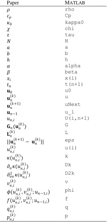
The mathematical quantities and the corresponding variables used in the MATLAB code are shown in Table 1.
Paper MATLAB
𝜌 rho
𝑐𝑝 Cp
𝜅0 kappa0
𝜒 chi
𝜏 tau
𝑁 N
𝑎 a
𝑏 b
ℎ h
𝛼 alpha
𝛽 beta
𝑥𝑖 x(i)
𝑡𝑛 t(n+1)
𝐮0 u0
𝐮𝑛
(𝑘) u
𝐮𝑛(𝑘+1) uNext
𝐮𝑛−1 u_1
𝑢𝑛,𝑖 U(i,n+1)
𝐆𝑛(𝐮𝑛 (𝑘)
) G
𝐋(𝑘)𝑛 L
||𝐮𝑛 (𝑘+1)
− 𝐮𝑛 (𝑘)
|| eps
𝑢𝑛,𝑖(𝑘) u(i)
𝜅(𝑢𝑛,𝑖(𝑘)) k
(𝑘) Dk
1 1.5
2 2.5
3
0 5 10 15
0 0.5 1 1.5 2
1 1.2 1.4 1.6 1.8 2 2.2 2.4 2.6 2.8 3 0.4
9. Acknowledgement
This research was carried out in the ELTE Institutional Excellence Program (1783-3/2018/FEKUTSRAT) supported by the Hungarian Ministry of Human Capacities, and supported by the Hungarian Scientific Research Fund OTKA, No. K112157 and SNN125119
10. References
[1] R.B. Bird, W.E. Stewart, E.N. Lightfoot, Transport Phenomena, 2nd Edition, John Wiley & Sons, Inc., (2002) [2] H.S. Carslaw, J.C. Jaeger, Conduction of Heat in Solids, 2nd
Edition, Oxford University Press, (1986)
[3] S.L. Sobolev, Partial Differential Equations of Mathematical Physics, Dover Publications, (1989)
[4] J. Lienemann, A. Yousefi, J.G. Korvink, Nonlinear Heat Transfer Modeling, In: P. Benner, D.C. Sorensen, V. Mehrmann (eds) Dimension Reduction of Large-Scale Systems, Lecture Notes in Computational Science and Engineering, 45 (2005) 327-331 [5] U.M. Ascher, S.J. Ruuth, R.J. Spiteri: Implicit-Explicit
Runge-Kutta Methods for Time-Dependent Partial Differential Equations, Appl Numer Math, vol. 25 (2-3) (1997)
[6] U.M. Ascher, R.M.M. Mattjeij, R.D. Russel, Numerical Solution of Boundary Value Problems for Ordinary Differential Equations, in: Classics in Applied Mathematics, vol. 13, SIAM, (1995) [7] S.M. Filipov, I.D. Gospodinov, I. Faragó, Shooting-projection
method for two-point boundary value problems, Appl. Math. Lett. 72 (2017) 10-15