Volume 2009, Article ID 945717,14pages doi:10.1155/2009/945717
Research Article
Adapted Active Appearance Models
Renaud S´eguier,
1Sylvain Le Gallou,
2Gaspard Breton,
2and Christophe Garcia
21SUP ´ELEC/IETR, Avenue de la Boulaie, 35511 Cesson-S´evign´e, France
2Orange Labs—TECH/IRIS, 4 rue du clos courtel, 35 512 Cesson S´evign´e, France
Correspondence should be addressed to Renaud S´eguier,[email protected]
Received 5 January 2009; Revised 2 September 2009; Accepted 20 October 2009
Recommended by Kenneth M. Lam
Active Appearance Models (AAMs) are able to align efficiently known faces under duress, when face pose and illumination are controlled. We propose Adapted Active Appearance Models to align unknown faces in unknown poses and illuminations. Our proposal is based on the one hand on a specific transformation of the active model texture in an oriented map, which changes the AAM normalization process; on the other hand on the research made in a set of different precomputed models related to the most adapted AAM for an unknown face. Tests on public and private databases show the interest of our approach. It becomes possible to align unknown faces in real-time situations, in which light and pose are not controlled.
Copyright © 2009 Renaud S´eguier et al. This is an open access article distributed under the Creative Commons Attribution License, which permits unrestricted use, distribution, and reproduction in any medium, provided the original work is properly cited.
1. Introduction
All applications related to face analysis and synthesis (Man-Machine Interaction, compression in video communication, augmented reality) need to detect and then to align the user’s face. This latest process consists in the precise localization of the eyes, nose, and mouth gravity center. Face detection can now be realized in real time and in a rather efficient manner [1,2]; the technical bottleneck lies now in the face alignment when it is done in real conditions, which is precisely the object of this paper.
Since such Active Appearance Models (AAMs) as those described in [3] exist, it is therefore possible to align faces in real time. The AAMs exploit a set of face examples in order to extract a statistical model. To align an unknown face in new image, the models parameters must be tuned, in order to match the analyzed face features in the best possible way. There is no difficulty to align a face featuring the same characteristics (same morphology, illumination, and pose) as those constituting the example data set. Unfortunately, AAMs are less outstanding when illumination, pose, and face type changes. We suggest in this paper a robust Active Appearance Model allowing a real-time implementation. In
the next section, we will survey the different techniques,
which aim to increase the AAM robustness. We will see that none of them address at the same time the three types
of robustness, we are interested in pose, illumination, and identity. It must be pointed out that we do not consider the robustness against occlusion as [4] does, for example, when a person moves his hand around the face.
After a quick introduction of the Active Appearance Models and their limitations (Section 3), we will present our
two main contributions in Section 4.1in order to improve
AAM robustness in illumination, pose, and identity.
Exper-iments will be conducted and discussed inSection 5before
drawing a conclusion, suggesting new research directions in the last section.
2. State of the Art
We propose to classify the methods which lead to an increase of the AAM robustness as follows. The specific types of dedicated robustness are in italic.
(i) Preprocess
(1) Invariant features(illumination) (2) Canonical representation(illumination)
(ii) Parameter space extension
(1) Light modeling(illumination)
(iii) Models number increasing
(1) Supervised classification(pose/expression) (2) Unsupervised classification(pose/expression)
(iv) Learning base specialization
(1) Hierarchical approach(pose/expression) (2) Identity specification(identity)
Preprocessmethods seek to substitute the AAM texture
input for a preprocessed image, in order to minimize the
influence of illumination. In Invariant features, an image
feature invariant, or a less illumination sensitive variation, is used: an image gradient [5], specific face features like corner detectors for the eyes and mouth [6], the concatenation of several colors components (H and S from HSV code and image gradient for example) [7], wavelet networks [8], or
distance map [9]. Except for the last one, those methods
all have a serious drawback: by concatenating the different invariant characteristics, they increase the texture size and therefore the algorithm complexity. Steerable filters [10] can be used to replace texture information and to characterize the region around each landmarks. The evaluation of those filters increases the algorithm complexity but the amount of information to be process by the AAM remains the
same if low resolution models (64×64) are used for
real-time application. For high resolution models, a wedgelet representation is proposed [11] to compress the texture. In
a Canonical representation, the illumination variations are
normalized [12] or reduced [13]. The shadows also can
be evaluated [14], in order to recover the face 3D model,
and then reproduce a texture without any shadow. Those approaches remain uncertain.
Parameter Space Extensionmethods increase the number
of AAM parameters, in order to model the variability introduced in the learning base, which was used to create the
face model. InLight modeling, a subspace in the parameter
space is learned and built, in order to control the illumi-nation variation. A modeling throughout the Illumiillumi-nation Cone [15, 16] or Light Fields [17, 18] is suggested. The illumination direction can also be estimated through the construction of a learning base of faces, which were acquired
under a number of different illuminations, each of them
being created by the variation of a single light source position
[19]. The illumination variations are then modeled by the
principal component analysis embedded in the AAM. All of those methods make the algorithm cumbersome, since the number of parameters needing optimization is increased, and the parameter space is broken up. The optimization, carried on a bigger and noncompact space parameter, is
then more difficult to control. In 3D modeling, the face
pose variability is transferred from the appearance parameter space to the sub-space which controls the pose (face position
and angle). Reference [20] introduces a new parameter to
be optimized, using the pose information associated to each face represented in the learning base. A 3D AAM can also be used either from the shapes and textures acquired from
a scanner [21], or with a frontal and profile face view
of each of the learning base face [22–24]. Reference [25] enriches the 3D AAM’s parameters by using the Candide model parameters related to Action Units to deform the mouth and eyebrows. The 3D approach is clearly relevant to increase the AAM robustness related to the pose variability. Nevertheless, as the 3D model becomes more complex, a real-time implementation remains difficult.
Models number increasing methods specify the classes
existing in the parameter space of the AAM parameters and define a specific active model in each of those classes. In Supervised classification, the variability type of the learning base is defined and the classes which make up the parameter
space are known: the different face views used for the
pose variability [26–29] or the different expressions for the
expression variability [30]. A huge model containing each
submodel specific to each view can be constructed [31] by
concatenating each shape and texture vectors for each view
on two large shape and texture vectors. In Unsupervised
classification, the classes which constitute the parameter space
are found automatically via K-means [32] or a Gaussian
mixture [33,34]. For each of these methods, active models are numerous. They must be optimized in parallel, in order to decide which one is best suited for the analyzed face. This is not feasible in real time, in our applicative context. One single model can be used in conjunction with Gaussian
mixture [35] to avoid implausible solution during the AAM
convergence.
Learning base specializationmethods restrict the search
space to only one variability (of one face feature or identity).
In Hierarchical approach, face features research is divided
in two steps: a rough research of face key points and then a refined analysis of face feature by the mean of a specific model for each face feature (eyes, nose, mouth) [36–39]. Like the previous methods, those approaches consist in increasing the number of active models to be optimized in parallel, and then make the alignment system cumbersome.
In Identity specification, the database identity variability is
removed. Reference [15] claims that a generic AAM featuring pose, identity, illumination, and expression variability is less
efficient than an AAM dedicated to one identity featuring
only pose, illumination, and expression variability. Reference [40] suggests to perform an on-line identity adaptation on an image sequence, by means of a 3D AAM construction, starting from the first image of the face without any expression. This method is not robust since the first image must be perfectly aligned to allow a good 3D AAM modeling. None of those methods fulfill our constraints, since none of them take into account unknown faces in variable pose and illuminations, at the same time. Let us recall that our main objective is to keep the AAM real-time aspect, while increasing their robustness. Therefore, we started
with Invariant features methods related to illumination
robustness, in which the AAM texture is pre-processed, and then later suggested a technique (Section 4.1), which does not increase the AAM computation cost. With regard to the robustness associated with pose and identity, and consid-ering the work presented inIdentity specificationas a start point, we propose to adapt the active model to the analyzed
3. Imitation of Active Appearance Models
3.1. Modeling. Active Appearance Models (AAMs) create a
joint model of an object’s texture and shape from a database comprising different viewsIiof the object. The texture inside
the shape si is normalized in shape (by means of mean
shape warping) and in luminance (by means of gray levels mean and variance) and leads to a free shape texturegi. Two
Principal Component Analyses (PCA) are performed on the shapes and textures examples of the learning base
si=s+Φs∗bsi,
gi=g+Φg∗bgi.
(1)
sandgare the mean shape and mean texture,ΦsandΦg
are both vectors representing the variations of the orthogonal modes related to shape and texture, respectively.bsiandbgi
are both vectors representing shape and texture parameters. We then apply a third PCA on vectorsb=[bsi|bgi].
bi=Φ∗ci. (2)
Φ is the matrix of the eigenvectors obtained by PCA.
ciis the appearance parameters vector. To each eigenvector
is associated an eigenvalue, which indicates the amount of deformation it can generate. In order to reduce the vector
cdimension, we keep 99% of the model deformation. It is
then possible to synthesize an image of the object with the appearance vectorc.
3.2. Segmentation. When we want to align the object in an
unknown imagei, we shift the model defined by the vectorc
relating to a pose vectort:
t=θ,S,tx,ty t
. (3)
θ is the rotation of the model in the image plan, S is
the scale, andtx andty are, respectively, the gravity centre
abscissa and ordinate of the model in the analyzed image. We adjust step by step each component of vectorc, creating then at each iteration a new shapexm, and a new texturegm
both normalized in shape and luminance, respectively. Let us now consider the texturegiraw associated with the region of
the imageIi inside the shapexm. We warp this texture into
the mean shapes(1) thanks to the warping functionW (4),
and we perform a photometric normalization (5) using the
meangiraw/sand varianceσ(giraw/s) evaluated on the warped
texturegiraw/s. The residual error δg between the texturegi
extracted from the image, and the texturegmgenerated by the
model is then minimized throughout the model parameters tuning, by means of a pre-computed Jacobian, which links the errors to the appearance and pose vectors variations [3],
or by applying classical optimization techniques like simplex [41] or gradient descent [42]
giraw
s =W
⎛ ⎜ ⎜ ⎝g iraw
si
,c
⎞ ⎟ ⎟
⎠, (4)
gi=giraw/s−giraw/s
σgiraw/s
, (5)
δ=gi−gm avec delta=[δ1· · ·δi· · ·δN, ]t (6)
withNbeing the number of pixels inside the texture. After
a number of iterations, typically one hundred, the errorepix
(7) converges to a small value: the model overlaps the object in the imageIi, and produces an estimation of its shape and
texture. Those steps are summarized inAlgorithm 1
epix= 1
N
N
i=1
δi2. (7)
Algorithm 1. Classical-AAM Segmentation.
(1) Image acquisition
(2) Optimization. Repeat (a) to (e)
(a) From the model, generate a shape xm and a
texturegm
(b) Retrieve a nonnormalized texture giraw in the
image
(c) Normalizegirawto producegi:
(i) Warpgirawin the mean shape(4)
(ii) Photometric normalizegiraw(5)
(d) Evaluate the errorgi−gm(6)
(e) Tune the model parameters
The numberNoptim of operations, which are processed
during the optimization step (see (8)), is evaluated from
the number N, which is the number of texture pixels,
thec appearance vector dimensionNc and theNPts points
which make up the shape.Noptimdoes not take into account
the warping (Algorithm 1 (c).(i)): it is realized on the
GPU, and uses 50% of the total processing time (a CPU warping implementation will reduce the process speed by one hundred)
Noptim≈N
8 3Nc+ 12
+NPts(2Nc+ 17) + 4Nc2. (8)
3.3. Robustness. AAM robustness is then linked to the
(a)
−0.5 0 0.5 1
c
(2)
−1 −0.5 0 0.5 1 c(1)
(b)
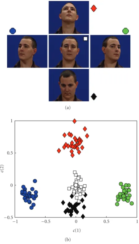
Figure1: Multimanifold in the parameter space.
data, will appear. Consequently, it is very difficult to force
the AAM to converge in this breaking up space. Figure 1
illustrates this problem. The learning base is realized from thirty faces in five different poses. The projection of those examples on the two first appearance parameters shows clearly four clusters, with each of them being specific to a particular pose. Only the frontal faces and those oriented towards the bottom seem to belong to the same cluster. The manifold in this example is clearly broken up; leading thus to a multi-manifold.
4. Proposed Methods
Our two main contributions consist of the Oriented Map Active Appearance (OMAP) Models to give AAM the capacity to align the face in any illumination conditions; the Adapted AAM for pose and identity robustness.
4.1. OM-AAM: Oriented Map Active Appearance Models.
Empirical comparisons in face recognition [43] show that
among thePre-processmethods (seeSection 2), the uniform
or specific histogram transformations are those which lead to the best recognition rates. For that reason, we propose to apply systematically on the images an adaptive histogram equalization from CLAHE [44]. It consists in splitting the image in eight by eight blocks, and in realizing in each block a specific histogram equalization according to a Rayleigh distribution. A specific equalization function is then attached to each block. In order to be able to reject the side-effect related to each blocks, the final result for each pixel is the bilinear interpolation of the equalization functions, associated to the four neighboring blocks of the evaluated pixel
I1
x,y=CLAHEI0
x,y. (9)
A comparison [45] between the Viola and Jones face
detector [2] and Froba’s one [46] shows that their relative performances are equivalent when the background is uni-form. The first detector is more efficient when faced with a complex background, but is also more difficult to implement. In our application, faces are previously detected and we must align them. The background does not disturb very much the AAM performances.
For that reason, we started with the works of [46,47]. These explain how to create, with the original image, two images representing the sines and cosines of the detected
angle on each pixel, with the work of [5], which explains
how to generate two images with both horizontal and vertical gradients. We propose to simply use the angle on each pixel instead of its gray level. This angle is evaluated onNavalues.
In practice we quantify it on eight bits, soNa=255. Under
a quantification of six bits the results begin to decrease. The new texture is then made out of an image representing the orientation of each pixel, that we call an oriented map. If
Gx andGy represent the horizontal and vertical gradients
evaluated on the image I1, then the oriented map, whose
values evolve between 0 and 2Π, is estimated in the following manner:
I2
x,y=Na
2 ·
1 + 1
Π·atan2
Gy
x,y Gx
x,y
. (10)
The function atan2 is the fourth quadrant inverse
tangent. As we can see inFigure 2, when the edges are coded between 0 and 2Π, a discontinuity exists in 0. The roughly vertical edges generate at the same time very low and high levels of information in the oriented map. We observe the effect of this discontinuity on the right face outline (see Figure 3) which flickers between black (high part of the face outline) and white (low part). We propose to realize a mapping (11) from [0..2Π] to [0..Π/2] with modNa/2the
moduloNa/2 operation, andabsthe absolute value
I3
x,y=Na
4 −abs
modNa/2
I2
x,y−Na
4
π
0
255
3π/2
3π/2 π/2
64
0 0
π 2π
2π 0 π/2
Figure2: Mapping from [0..2Π] to [0..(Π/2)].
As we can see inFigure 2, after the mapping process, the edges close to the vertical (orientation angle close to zero, Πor 2Π) will get a low level of information on an oriented map and those, close to an horizontal position (orientation angle close to Π/2 or 3(Π/2)), will produce a high level of information.
In order to reduce the noise in uniform regions as
illustrated in the background of Figure 3(c), we propose
to emphasize the signal correlated with the high gradient information region, as it is suggested by [5] and to use the following nonlinear function f:
f(G)= G
G+G withG=
Gx
x,y2+Gy
x,y2 (12)
with G being the mean of G. Figure 3(d)represents f(G)
evaluated on the texture ofFigure 3(a)
I4
x,y= f(G)· ∗I3
x,y (13)
with·∗being the element by element multiplication. During
the modeling, the oriented textures from images I4 will
replace the textures usually used by the AAM.
In the segmentation phase, we evaluate the difference
between the texture synthesized thanks to the model and the texture analyzed in the image (Figure 3(f)). This texture, in classical AAM, is normalized in luminance and shape at each iteration. The photometric normalization is no longer necessary in our case, since the new texture results in an angle evaluation. When the object is oriented with an angle of θ, we shift the model with respect to the vector t (3) and evaluate a difference between the original image inside the model obtained shape, and the model obtained texture.
The difference between those two textures is made in the
reference model: a normalized shape with an orientation
θ=0.
This is not a problem when we deal with gray levels. In our case, since we have replaced the pixel information by the edges orientation, which is evaluated for each pixel, there is no more rotational invariance. As an example, let us consider the ellipse lying inFigure 4with a pixelPmodelon a 45-degree
edge. On an oriented map (Figure 4(a)), this pixel in the
reference model will have a value of 45 (if the levels range from 0 toNa =90). If we look at the same rotated ellipse of
−45 degrees in a test image (Figure 4(b)), the corresponding
pixelPimage on the object will have a null value, since the
filters used in order to extract the gradients work in the same direction, despite the object orientation. After the warping
which takes into account the pose parameter θ = −45,
the texture of the rotated object will have the same value
before and after rotation. The corresponding pixel p in the
model (Pmodel=45) will be compared to the image’s p pixel
(Pimage=0).
In order to compare the model texture to that of the object despite its orientation in the image, we simply subtract, before that comparison, an offset (14) to the levels
produced by the oriented map. This offset is linked to the
pose parameterθin the following manner:
Ofset=floor
Na∗ θ
2∗pi
. (14)
We can see in Figure 4(c) that this operation allows
the comparison of the orientation information lying in the model texture and the analyzed image texture, whatever the object orientation is.
In order to be able to subtract the offset (14), we need to keep the original values of the edge angle, detected in the image. Therefore, we propose to evaluate, during the
segmentation phase, the oriented map between 0 and 2πin
the pre-process step (Algorithm 2(2).(b)), and to realize at each iteration, during the optimization phase, the mapping (Algorithm 2 (3).(c).(ii)) and the product (Algorithm 2 (3).(c).(iii)) operated by the nonlinear functionf. This func-tion is evaluated during the pre-process (Algorithm 2(2).(c)) and is, then, not time consuming. This new segmentation
proposition is summarized by the followingAlgorithm 2.
Algorithm 2. OM-AAM segmentation
(1) Image acquisition
(2) Pre-process
(a) Histogram equalization (CLAHE)(9)
(b) Oriented map generation: angle range from 0 to 2π(10)
(a) (b) (c)
(d) (e) (f)
Figure3: (a)I0, (b)I2, (c)I3, (d)f(G), (e)I4, (f) oriented texture.
Pmodel Pmodel
(a)
Pimage Pimage
(b)
Pimage Pimage
(c)
Figure4: Ellipse model (a), ellipse texture in the tested image without offset (b), ellipse texture in the tested image with offset (c). The
second line is a zoom of the first one.
(3) Optimization. Repeat (a) to (e)
(a) On the basis of the model, generate a shapexm
and a texturegm
(b) Retrieve a nonnormalized texture giraw in the
image
(c) Normalizegirawto producegi:
(i) Add the offset angle to the texture(14)
(ii) Map the orientation from [0..2Π] to
[0..Π/2](11)
(iii) Multiply each pixel by the nonlinear func-tion evaluated in step (2).(c)
(iv) Warp the new texture in the mean shape to producegi
(d) Evaluate the errorgi−gm
(e) Tune the model parameters.
The cost overrun generated by the oriented map is in the order of 9Noperations. In real context, we use a texture of
N = 1756 pixels and a shape ofNPts = 68 key points for
an appearance vector comprising approximately Nc = 10
parameters (see (8)). The optimization cost overrun is 11%, bearing in mind that the warping consumes fifty percent
of the process time. In our implementation, we effectively
observe a similar increase (13.5% to be precise) when we
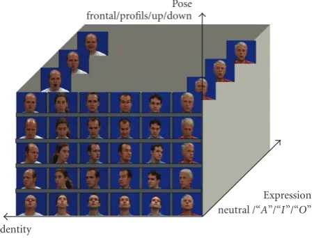
Identity
Pose frontal/profils/up/down
Expression neutral /“A”/“I”/“O”
Figure5: General database.
4.2. Adapted-AAM. As previously said in Section 3.3, the
AAM robustness is related to the face variability in the learning base. A great variability induces a multi-manifold parameter space which disturbs the AAM convergence. Instead of using a very generic model containing a lot of
variability, we suggest to use an initial model M0, which
contains only a variability in identity, and then use a
specific model Madapt, containing variability in pose and
expression.
4.2.1. Initial Model. Let a general database contain three
types of variability: expression, identity, and pose (see Figure 5). We do not include illumination variability in this database since this variability was treated in the preceding sections. It is made of several different faces, holding four distinct expressions:neutral,A,I, andO. Each of the faces presents each of those expressions for the five different poses: frontal face, looking up, left, right, and looking down.
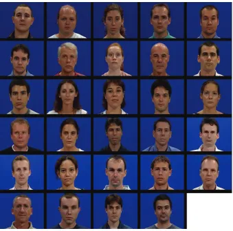
The initial modelM0 is realized from a databaseBDD0
containing different neutral expression frontal faces (see
Figure 6). We use only the images on the horizontal axis of the general database. This initial model will be used to perform a rough alignment on the unknown face.
4.2.2. Type Identification of the Analyzed Face. LetC0be the
appearance vector after the alignment of the modelM0on the
unknown analyzed face. In the parameter space of the model
parameters, we seek for theknearest parameters vectors of
C0 belonging to the learning initial databaseBDD0. Those
k nearest neighbors correspond to the k nearest faces of
the analyzed one. The metric used is simply the Euclidean
distance in the parameter space. For example in Figure 7,
the vectorCp will identify the face number p as being the
most similar to the analyzed one. Theknearest models will
correspond in the initial databaseBDD0to specific identities,
which are the most similar to the identity of the unknown analyzed face.
4.2.3. Adapted Model. From this set of knearest identities,
we generate an adapted database BDDadapt containing the
corresponding faces in different expressions and poses.
BDDadapt is a subset of the general database (Figure 5). Figure 8illustrates such an adapted database whenk=1.
FromBDDadapt, we generate the adapted modelMadapt.
Whenk = 1, 2, or 3, it is possible to evaluate beforehand
the adapted model, depending on the number of different
faces in the general database. Fork = 1 this database can
contain up to one hundred faces, since the total number of combinations is around five thousands, and 2.5 GB will then be sufficient to store the five thousand models. Ifk=3 then comparatively small general database will be used, that is, 33 different faces if only 2.5 GB memory is available in the system.
4.2.4. Implementation. When we need to align an unknown
face in a static image, we then simply align the face with the
initial modelM0and apply the pre-computed model, which
corresponds to theknearest faces. If a video stream related to one person needs to be analyzed, we use the first second of the stream in order to perform a more robust selection of the adapted model. On the first images, we align the face with the initial modelM0. We evaluate the errorepix (7) on each
image. This error is remarkably stable, because of the use we make of the oriented map; it is then possible to compare it to a threshold, in order to decide if the model has converged.
We then evaluate, from the correctly aligned faces, the k
nearest identities which must be taken into account in the general database, in order to construct the adapted model. This model is then used on the following images in the video stream, in order to align the face.
5. Experiments
We will specify hereafter the parameters values and metric to evaluate the performances of our two contributions (OM-AAM and Adapted (OM-AAM). This section will end with a discussion on the different results.
5.1. Experiments Setup. We use the same metric as in [48], in
order to evaluate the error,
e= 1
M·Deye
M
j=1
ej, (15)
where ej is the error made on one of the M = 4 points
representing the eyes, nose, and mouth centers;Deye is the
distance between the eyes. In the context of the robustness analysis to illumination, identity, and pose, those four points are sufficient to illustrate the performances of our proposals. The precision of the ground truth is roughly 10% of the distance between the eyes of the annotated faces; beyond
e=25%, we consider that the alignment is not correct. We
Figure6: Initial databaseBDD0.
Cp
C0
Reduced space Initial baseNneutral
and frontal faces
Figure7: Nearest model identification.
regard to the oriented map, no specific parameterization is necessary: the orientation number (Na) is quantified on
height bits and is not related to the type of the testing base images.
5.2. OM-AAM Performances. Let us remember that our
objective is to make the AAM robust to illumination variations without any increase in the processing time.
The DM-AAM of [9] complies with our constraints. We
then propose to illustrate the OM-AAM performances, in comparison to those of the DM-AAM and classical AAM. Those comparisons will be made in a generalization context: the faces used to construct the model (18 persons from the
M2VTS database [49]) and the ones used for the tests come
from distinct databases.
Most of the time, a process which increases the robust-ness of an algorithm in a specific case decreases its per-formances in standard cases [43]. For that reason, we will test our suggestions on a database, which is dedicated to illumination problems (CMU-PIE: 1386 images of 66 faces under 21 different illuminations [50]) and on an other one representing different faces with several expressions taken
in different backgrounds (BIOID: 1521 images [51]) under
variable light exposition (seeFigure 9). This latest database
is more difficult to process, since the background can be
different and the faces present various positions, expressions and aspects. People can have glasses, moustaches, or beard.
Figure 10represents the percentage of the images, which
have been aligned with the error e (15). For example the
Figure8: Adapted databaseBDDadapt.
Figure9: Image examples of BIOID (top) and CMU-PIE (bottom) databases.
the test images, the centers of the mouth, eyes, and nose were detected with a precision less or equal to 15% of the distance between the eyes of the analyzed face. The DM-AAMs are more powerful than the classical ones when used with normalized faces with variable illuminations (CMU-PIE database), but are useless in standard situations (BioId database). The DM-AAM uses a distance map, which is extracted from the image contours points. The threshold used to detect the contours point is crucially important, and is based on the assumption that all testing base images share the same dynamic. This is not the case of the BioId database, in which the image contrasts present a great variation. Conversely, OM-AAMs do not use any threshold, since we do not extract any edge information but the gradient information on each pixel of the image.
A reference point used in the state of the art technology is often the point of abscissa 0.15. On the CMU-PIE database, OM-AAMs are able to align 94% of the faces with a precision less or equal to 15%, when DM-AAM and classical ones
are less efficient: their performances are, respectively, 88% and 79%. But when the faces are acquired in real situations, our proposition overcomes other methods: in the BIOID database, OM-AAM can align 52% of the faces with a precision less or equal to 15%, which represents a 27 and 42% performance gain, with regard to classical AAM and DM performances, respectively.
5.3. Adapted AAM Performances. We propose to test the
adapted AAM on the static images of the general database
BDD0 (Figure 5). A test sequence is then made, with one
unknown person presenting four expressions under five different poses; the learning base associated to this testing base is made of all the other persons. A cross-validation of
type Leave-one-out is used. All faces are tested separately,
using all the other ones for the learning base. All the faces of the database have been tested, representing at the end a set of 580 images with a big variety of poses, expressions, and identity. The initial database used to generate the initial
model M0 is the same as the one presented in Figure 6,
apart from the fact that the testing face has been removed.
It contains then 28 different faces. This model is applied
0 0.1 0.2 0.3 0.4 0.5 0.6 0.7 0.8 0.9 1
Con
ver
ge
n
ce
ra
te
(%
)
0.1 0.15 0.2 0.25
Error OM-AAM
DM-AAM Classical AAM
CMU-PIE
(a)
0 0.1 0.2 0.3 0.4 0.5 0.6 0.7 0.8 0.9 1
Con
ver
ge
n
ce
ra
te
(%
)
0.1 0.15 0.2 0.25
Error OM-AAM
DM-AAM Classical AAM
BIOID
(b)
Figure10: Comparative performances of the three tested alignment algorithms on CMU-PIE and BIOID databases. The convergence rate specifies the percentage of the images in the testing base being aligned with a specif error (15) given by the abscissa value.
To be able to find the optimal parameter k, we have
tested our algorithm for differentkvalues within the range [1· · ·28].Figure 11shows the percentage of the face aligned with a precision less or equal to 15% of the distance between
the eyes, versusk: the number of nearest faces. As we can
see, in the range [3· · ·10], the alignment performances are
relatively stable. They collapse after k = 15; the adapted
model is based on fifteen faces in five poses and four different expressions. The parameter space is breaking up leading to a
0.75 0.8 0.85 0.9 0.95 1
Con
ver
ge
n
ce
ra
te
(%
)
0 5 10 15 20 25
knearest faces
Figure11: Adapted AAM performances for an error of 15% versus the number of the nearest faces used to construct the adpated model.
multi-manifold, and optimization becomes more difficult to
conduct (cf.Section 3.3).
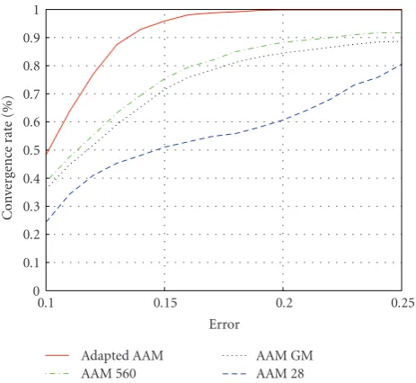
We compare the performances of our system when
k = 2 (Adapted AAM) to those of three others different
AAM. The first one (AAM 28) gets identity as the only variability and is made of the 28 faces (the twenty-ninth being tested) in frontal view and neutral expression. The second one (AAM 560) is full of rich variability, since it is based on 560 images representing 28 faces, representing themselves four expressions under five different poses. Lastly the third one (AAM GM) [35] (seeSection 2) uses Gaussian mixtures to specify the regions of plausible solutions in the parameter space (seeFigure 13). It is interesting to compare our proposition to this method since it is dedicated to multi-manifold spaces. We cannot implement it on a restricted database like the one of “AAM 28” which represents only one cluster of frontal faces. Four Gaussians were used to catch the density on the 560 images of the rich database of “AAM 560” model. We use the three first components of the appearance vector as it was indicated by the authors since the density in the other dimensions is uniform.
5.4. Adapted AAM Performances Discussion. The algorithmic
one second we switch to tracking mode: only five positions are tested around the center of the face so the algorithm works at 21 Hz. If the dimensionNcof the appearance vector
(see (8)) is multiplies by ten, then the number of operations is rougthly multiplied by ten too, with the warping time being not affected by this dimension growth. Even in tracking mode, this increase will then lead to only a 2 Hz framerates
for “AAM 560” or “AAM GM” which is not sufficient for real
time applications.
Figure 12shows the superiority of the “Adapted AAM” over the three other models. The performances of the “AAM 560” are less good than those of the “Adapted AAM.” It is consistent with the fact that the database used to build the “AAM 560” is much more rich in variability: the parameter space of this latest model is split into multi-manifolds. The “AAM GM” is able to identify these manifolds but is still slightly less good as “AAM 560,” that will be discussed hereafter.
If we look at the reference error (15%), then our proposition is ten times more rapid than the “AAM 560” because of the dimension of the appearence vector, and
clearly more effective (performances improvment of 20%)
than the same heavy “AAM 560” model. If we compare now the “Adapted AAM” to the other light model (AAM 28), the “Adapted AAM” has the same complexity and is more
effective for 45% of the images of the testing base. As a
conclusion, our model is more rapid and effective than other models, because it has focused on a relevant database, which is related to the testing face.
To understand why the results of “AAM GM” are less good then the ones of “AAM 560” it is necessary to look at the trajectory used during the AAM convergence process. Figure 13 shows the four Gaussians which were found by the Expected Minimization algorithm to specify the density in the first three dimensions and the two trajectories of the solutions found by the two AAM during the convergence. Both of them are initialized in the middle of the space and of course have the same path in the beginning. After few iterations the “AAM GM” finds a solution in a region specified as empty and performs a gradient descent to go back in the best direction in a plausible solution region. For “AAM 560” part, it continues to reach the good cluster and nearby it tries to find the best solution. As illustrated byFigure 14(a zoom onFigure 13), each time the classical process of AAM proposes a nonplausible solution to the “AAM GM,” it tries to go back, for that reason the trajectory of the “AAM GM” is disturbed compare to the “AAM 560” smooth trajectory. In fact [35] contribution was very interesting but illustrated only on one image as performance evaluation: two very different shapes of one object were to be fined. Maybe if the initialization point is in a region specified as non plausible, then after one iteration only, the gradient descent on the density charaterized by the Gaussians leads to a very fast convergence in the good cluster region and then the classical optimization is able to find a nice solution.
The trajectories end of Figures 13 and 14 lead to the
images (b) and (c) of Figure 15 . The associated models are based on the same 560 learning examples with very rich variability, so they are both able to catch the orientation of
0 0.1 0.2 0.3 0.4 0.5 0.6 0.7 0.8 0.9 1
C
o
n
ve
rg
en
cer
at
e(
%
)
0.1 0.15 0.2 0.25
Error Adapted AAM
AAM 560
AAM GM AAM 28
Figure12: Comparative performances of “Adapted AAM,” “AAM 560”, “AAM GM,” and “AAM 28”. The convergence rate specifies the percentage of the images in the testing base being aligned with a specif error (15) given by the abscissa value.
−1 −0.8 −0.6 −0.4 −0.2 0 0.2 0.4 0.6 0.8 1
c
(2)
−1 −0.5 0 0.5 1 1.5 c(1)
Figure13: Parameter space density estimation by Gaussian mix-tures.
the face. It is interesting to note that the shape found by
the “AAM GM” (Figure 15(c)) is more natural than the one
−0.2 −0.1 0 0.1 0.2 0.3
c
(2)
−0.2 −0.1 0 0.1 0.2 0.3 0.4 0.5 0.6 0.7 c(1)
AAM GM AAM 560
Figure14: AAM GM and AAM 560 trajectories in the parameter space.
(a) (b)
(c) (d)
Figure15: Visual performances. Adapted AAM (a), AAM 560 (b), AAM GM (c), and AAM 28 (d).
Adapted AAM (Figure 15(a)) is the only method capable to produce a shape without any discontinuity, in the good orientation and a well placed nose.
6. Conclusion and Perspectives
Active Appearance Models are very efficient to align known
faces in constraints conditions (face pose and illumination). In order to make them robust to illumination variations, we have proposed a new AAM texture type and a new normalization during the optimization step. In order to make them robust to unknown faces moving in unknown poses in different expressions, we have suggested an adapted model. This adaptation is made by choosing, in a set of pre-computed models, the best suited model to the unknown
face. Tests made on public and private databases have shown the interest of our propositions; it is now possible to align unknown faces in nonconstraint situations, with a precision,
which is sufficient enough for most applications requiring
an alignment process (face recognition, face gesture analysis, cloning). Unlike [40] (cf.Section 2), where a specific model is made out of the first image of a video stream, we seek for the model which is best suited to the unknown face. This difference is significant; an imperfect initial alignment has no definitive repercussions. Our system is then more robust in view of the errors made by the initial generic model. At last, it is to be noted that the Adapted-AAM with oriented texture
offers the same computational complexity as the classical
AAM; they can be implemented in real time.
For emotion analysis and lip-reading, it is necessary to have a very precise alignment in order to be able to track the face dynamic. Precisely, the alignment performances must be evaluated on the localization of several points around the eyes, eyebrows, and mouth and not only on their gravity centers. We are now working on an adapted and hierarchical AAM, which use for each face characteristics (eyes and mouth essentially), the most relevant adapted model.
References
[1] C. Garcia and M. Delakis, “Convolutional face finder: a neural architecture for fast and robust face detection,”IEEE Transactions on Pattern Analysis and Machine Intelligence, vol. 26, no. 11, pp. 1408–1423, 2004.
[2] P. Viola and M. J. Jones, “Robust real-time face detection,”
International Journal of Computer Vision, vol. 57, no. 2, pp. 137–154, 2004.
[3] T. F. Cootes, G. J. Edwards, and C. J. Taylor, “Active appearance models,” inProceedings of the European Conference on Com-puter Vision (ECCV ’98), 1998.
[4] R. Beichel, H. Bischof, F. Leberl, and M. Sonka, “Robust active appearance models and their application to medical image analysis,”IEEE Transactions on Medical Imaging, vol. 24, no. 9, pp. 1151–1169, 2005.
[5] T. F. Cootes and C. J. Taylor, “On representing edge structure for model matching,” inProceedings of IEEE Computer Society Conference on Computer Vision and Pattern Recognition (CVPR ’01), vol. 1, pp. 1114–1119, 2001.
[6] I. M. Scott, T. F. Cootes, and C. J. Taylor, “Improving appearance model matching using local image structure,” in
Proceedings of the International Conference on Information Processing in Medical Imaging (IPMI ’03), pp. 258–269, 2003. [7] M. B. Stegmann and R. Larsen, “Multi-band modelling of
appearance,” in Proceedings of the Workshop on Generative Model-Based Vision (GMBV ’02), 2002.
[8] C. Hu, R. Feris, and M. Turk, “Active wavelet networks for face alignment,” inProceedings of the British Machine Vision Conference (BMVC ’03), 2003.
[9] D. Giri, M. Rosenwald, B. Villeneuve, S. Le Gallou, and R. S´eguier, “Scale normalization for the distance maps AAM,” inProceedings of the 9th International Conference on Control, Automation, Robotics and Vision (ICARCV ’06), Singapore, 2006.
Conference on Pattern Recognition (ICPR ’06), vol. 1, pp. 417– 420, 2006.
[11] S. Darkner, R. Larsen, M. B. Stegmann, and B. K. Ersboll, “Wedgelet enhanced appearance models,” in Proceedings of the Workshop on Generative Model Based Vision (GMBV ’04), Washington, DC, USA, July 2004.
[12] J. Zhu, B. Liu, and S. C. Schwartz, “General illumination correction and its application to face normalization,” in
Proceedings of IEEE International Conference on Acoustics, Speech and Signal Processing (ICASSP ’03), vol. 3, pp. 133–136, 2003.
[13] Y. Huang, S. Lin, S. Z. Li, H. Lu, and H.-Y. Shum, “Face alignment under variable illumination,” in Proceedings of IEEE International Conference on Automatic Face and Gesture Recognition (FGR ’04), pp. 85–90, 2004.
[14] W. Y. Zhao and R. Chellappa, “Illumination-insensitive face recognition using symmetric shape-from-shading,” in Pro-ceedings of IEEE Computer Society Conference on Computer Vision and Pattern Recognition (CVPR ’00), vol. 1, pp. 286–293, 2000.
[15] A. S. Georghiades, P. N. Belhumeur, and D. J. Kriegman, “From few to many: generative models for recognition under variable pose and illumination,” inProceedings of the Interna-tional Conference on Automatic Face and Gesture Recognition (FGR ’00), 2000.
[16] K.-C. Lee, J. Ho, and D. J. Kriegman, “Acquiring linear subspaces for face recognition under variable lighting,”IEEE Transactions on Pattern Analysis and Machine Intelligence, vol. 27, no. 5, pp. 684–698, 2005.
[17] R. Gross, I. Matthews, and S. Baker, “Fisher light-fields for face recognition across pose and illumination,” inProceedings of the German Symposium on Pattern Recognition, 2002.
[18] C. M. Christoudias, L.-P. Morency, and T. Darrell, “Light field appearance manifolds,” in Proceedings of the European Conference on Computer Vision, pp. 481–493, 2004.
[19] P. Kittipanya-ngam and T. F. Cootes, “The effect of texture representations on AAM performance,” inProceedings of the International Conference on Pattern Recognition (ICPR ’06), vol. 2, pp. 328–331, 2006.
[20] S. Romdhani, S. Gong, and A. Psarrou, “A multi-view nonlin-ear active shape model using kernel PCA,” inProceedings of the British Machine Vision Conference (BMVC ’99), pp. 483–492, 1999.
[21] V. Blanz and T. Vetter, “A morphable model for the synthesis of 3D faces,” in Proceedings of the International Conference on Computer Graphics and Interactive Techniques (SIGGRAPH ’99), pp. 187–194, Addison-Wesley, 1999.
[22] Y. Li, S. Gong, and H. Liddell, “Modelling faces dynamically across views and over time,” inProceedings of IEEE Interna-tional Conference on Computer Vision, vol. 1, pp. 554–559, 2001.
[23] J. Xiao, S. Baker, I. Matthews, and T. Kanade, “Real-time combined 2D+3D active appearance models,” inProceedings of IEEE Computer Society Conference on Computer Vision and Pattern Recognition (CVPR ’04), vol. 2, pp. 535–542, 2004. [24] A. Sattar, Y. Aidarous, S. Le Gallou, and R. S´eguier, “Face
alignment by 2.5D active appearance model optimized by simplex,” in Proceedings of the International Conference on Computer Vision Systems (ICVS ’07), 2007.
[25] F. Dornaika and J. Ahlberg, “Face model adaptation for tracking and active appearance model trainin,” inProceedings of the British Machine Vision Conference (BMVC ’03), 2003. [26] T. F. Cootes, K. N. Walker, and C. J. Taylor, “View-based
active appearance models,” inProceedings of the International
Conference on Automatic Face and Gesture Recognition (FGR ’00), pp. 227–232, 2000.
[27] T. F. Cootes, G. V. Wheeler, K. N. Walker, and C. J. Taylor, “Coupled-view active appearance models,” inProceedings of the British Machine Vision Conference (BMVC ’00), vol. 1, pp. 52–61, 2000.
[28] S. Z. Li, Y. Shuicheng, H. J. Zhang, and Q. S. Cheng, “Multi-view face alignment using direct appearance models,” in
Proceedings of the International Conference on Automatic Face and Gesture Recognition (FGR ’02), pp. 324–329, 2002. [29] C. Hu, R. Feris, and M. Turk, “Real-time wiew-based face
alignment using active wavelets networks,” inProceedings of the International Workshop on Analysis and Modeling of Faces and Gestures (AMFG ’03), 2003.
[30] X. Feng, B. Lv, and Z. Li, “Automatic facial expression recognition using both local and global information,” in
Proceedings of the Chinese Control Conference, pp. 1878–1881, 2006.
[31] C. R. Oost, B. P. F. Lelieveldt, M. ¨Uz¨umc¨u, H. Lamb, J. H. C. Reiber, and M. Sonka, “Multi-view active appearance models: application to X-ray LV angiography and cardiac MRI,” in
Proceedings of the International Conference on Information Processing in Medical Imaging (IPMI ’03), pp. 234–245, 2003. [32] Y. Chang, C. Hu, and M. Turk, “Probabilistic expression
analysis on manifolds,” in Proceedings of IEEE Computer Society Conference on Computer Vision and Pattern Recognition (CVPR ’04), vol. 2, pp. 520–527, 2004.
[33] C. Hu, Y. Chang, R. Feris, and M. Turk, “Manifold based anal-ysis of facial expression,” inProceedings of the Conference on Computer Vision and Pattern Recognition Workshop (CVPRW ’04), vol. 5, pp. 81–87, 2004.
[34] C. M. Christoudias and T. Darrell, “On modelling nonlinear shape-and-texture appearance manifolds,” inProceedings of IEEE Computer Society Conference on Computer Vision and Pattern Recognition (CVPR ’05), vol. 2, pp. 1067–1074, 2005. [35] T. F. Cootes and C. J. Taylor, “A mixture model for representing
shape variation,”Image and Vision Computing, vol. 17, no. 8, pp. 567–573, 1999.
[36] L. Zalewski and S. Gong, “2D statistical models of facial expressions for realistic 3D avatar animation,” inProceedings of IEEE Computer Society Conference on Computer Vision and Pattern Recognition (CVPR ’05), vol. 2, pp. 217–222, 2005. [37] Z. Xu, H. Chen, and S.-C. Zhu, “A high resolution
gram-matical model for face representation and sketching,” in
Proceedings of IEEE Computer Society Conference on Computer Vision and Pattern Recognition (CVPR ’05), vol. 2, pp. 470–477, 2005.
[38] G. Langs, P. Peloschek, R. Donner, and H. Bischof, “A clique of active appearance models by minimum description length,” inProceedings of the British Machine Vision Conference (BMVC ’05), pp. 859–868, 2005.
[39] Y. Tong, Y. Wang, Z. Zhu, and Q. Ji, “Facial feature tracking using a multi-state hierarchical shape model under varying face pose and facial expression,” inProceedings of the Interna-tional Conference on Pattern Recognition (ICPR ’06), vol. 1, pp. 283–286, 2006.
[40] U. Canzler and B. Wegener, “Person-adaptive facial feature analysis,” in Proceedings of the International Conference on Electrical Engineering, 2004.
[41] Y. Aidarous, S. Le Gallou, A. Sattar, and R. S´eguier, “Face align-ment using active appearance model optimized by simplex,” in
[42] M. B. Stegmann,Active appearance models: theory, extensions and cases, M.S. thesis, Informatics and Mathematical Mod-elling, Technical University of Denmark, DTU, Denmark, 2000.
[43] B. Du, S. Shan, L. Qing, and W. Gao, “Empirical comparisons of several preprocessing methods for illumination insensitive face recognition,” inProceedings of IEEE International Confer-ence on Acoustics, Speech and Signal Processing (ICASSP ’05), vol. 2, pp. 981–984, 2005.
[44] K. Zuiderveld, “Contrast Limited Adaptive Histogram Equal-ization,” inGraphics Gems IV, Academic Press, Boston, Mass, USA, 1994.
[45] D. Cristinacce and T. F. Cootes, “A comparison of two real-time face detection methods,” inProceedings of the Interna-tional Workshop on Performance Evaluation of Tracking and Surveillance, 2003.
[46] B. Froba and C. Kublbeck, “Robust face detection at video frame rate based on edge orientation features,” inProceedings of the 5th International Conference on Automatic Face and Gesture Recognition (FGR ’02), 2002.
[47] R. Belaroussi, L. Prevost, and M. Milgram, “Classifier combi-nation for face localization in color images,” inProceedings of the International Conference on Image Analysis and Processing (ICIAP ’05), pp. 1043–1050, 2005.
[48] D. Cristinacce and T. F. Cootes, “Feature detection and tracking with constrained local models,” inProceedings of the British Machine Vision Conference (BMVC ’06), 2006.
[49] Pigeon, “M2VTS Project,” M2VTS, 1996,
http://www.tele.ucl.ac.be/PROJECTS/M2VTS/m2fdb.html. [50] T. Sim, S. Baker, and M. Bsat, “The CMU pose, illumination,
and expression (pie) database,” inProceedings of the Interna-tional Conference on Automatic Face and Gesture Recognition (FGR ’02), 2002.