Article
A Practical Method for Assessing the Energy
Consumption & CO
2Emissions of Mass Haulers
Hassanean Jassim *, Weizhuo Lu and Thomas Olofsson
Department of Civil, Environmental and Natural Resources Engineering, Luleå University of Technology, Lulea 97187, Sweden; [email protected] (W.L.); [email protected] (T.O.)
* Correspondence: [email protected] or [email protected]; Tel.: +46-92-049-3463 or +46-70-298-3825
Abstract: Mass hauling operations play central roles in construction projects. They typically use many haulers that consume large amounts of energy and emit significant quantities of CO2. However, practical methods for estimating the energy consumption and CO2 emissions of such operations during the project planning stage are scarce, while most of the previous methods focus on construction stage or after the construction stages which limited the practical adoption of reduction strategy in the early planning phase. This paper presents a detailed model for estimating the energy consumption and CO2 emissions of mass haulers that integrates the mass hauling plan with a set of predictive equations. The mass hauling plan is generated using a planning program such as DynaRoad in conjunction with data on the productivity of selected haulers and the amount of material to be hauled during cutting, filling, borrowing, and disposal operations. This plan is then used as input for estimating the energy consumption and CO2 emissions of the selected hauling fleet. The proposed model will help planners to assess the energy and environmental performance of mass hauling plans, and to select hauler and fleet configurations that will minimize these quantities. The model was applied in a case study, demonstrating that it can reliably predict energy consumption, CO2 emissions, and hauler productivity as functions of the hauling distance for individual haulers and entire hauling fleets.
Keywords: hauling operations; optimum schedule; energy consumption; CO2 emission; hauler
1. Introduction
Road and highway construction are major undertakings that involve large-scale mass hauling operations. Haulers are designed to transport excavated material from cutting areas to filling areas or disposal areas during mass hauling operations. In the course of this work, they consume very large amounts of diesel fuel and emit large quantities of CO2 [1]. Previous research on hauling operations has largely focused on cost sensitivity analysis and reducing the execution costs of mass hauling operations (i.e., maximizing ‘productivity per unit cost’). There has thus been relatively little work on haulers’ energy consumption and CO2 emissions, despite their potentially significant impact on the local environment and global climate [2]. Zeng et al. [3] have shown that actors and decision-makers working with energy management systems have come under pressure to address a wide range of issues including energy consumption and the mitigation of greenhouse gas emissions. These authors also identified several regional and global environmental issues that are affected by energy activities.
equipment that is used and the way in which it is used [8]. Accordingly, reports published by the EPA’s Clean Air Act Scientific Advisory Committee in 2006 and 2008 showed that 7.5% of total CO2 emissions are generated by off-road equipment, with construction equipment accounting for 40% of these emissions [9]. As such, there is an urgent need for ways of maximizing the efficiency of mass hauling operations and for the widespread adoption of such methods within the construction sector. Many factors acting at different stages of the construction process contribute to the sector’s overall fuel consumption and emissions output, but the bulk of the emissions produced during road construction projects occur during the construction stage [10]. Mass hauling operations in road construction projects involve heavy haulers, which generally consume large quantities of energy; fuel costs account for around 30% of their total life-cycle costs [11]. More efficient allocation of haulers can significantly reduce both costs and emissions [12–14].
A few frameworks for reducing emissions from construction projects have been proposed. One, developed by Peña-Mora et al. [15], incorporates an emissions estimation model that can be used to determine which construction methods offer the best performance and lowest emissions. Lewis et al. [16] proposed a framework for estimating emissions due to excavation activities that can be used to control both costs and emissions. An analysis of emissions data conducted by Carmichael et al. [17] indicated that (under certain assumptions), procedures that minimize costs in earthmoving operations also minimize emissions. Subsequent analyses by the same authors emphasized the magnitude of the emissions generated by off-road haulers and reinforced the conclusion that designing earthmoving operations to minimize unit costs also minimizes unit emissions [18].
This paper presents a new model for estimating mass haulers’ energy consumption and CO2 emissions. The model depends on productivity rates for different hauler types, which are computed with a construction planning program using a bill of quantities for the various earthworking activities involved in road construction projects. The model’s output is then used to estimate the energy consumption and CO2 emissions of the chosen hauler fleet based on pre-determined hourly fuel consumption values for each hauler type included in the plan.
2. Literature Review
The energy consumption and emissions of mass hauling operations have been studied in some detail. However, much of this work has focused on building construction rather than road construction, even though both types of projects involve extensive earthwork activities and operations that account for a large proportion of the total energy consumption and CO2 emissions. The Swedish Transport Administration is working towards more energy efficient and environmental friendly infrastructure projects. Among others, the selections of construction materials and methods in the planning phase are regarded as an important aspect that may significantly influence the energy consumption and CO2 emissions in the life cycle of infrastructure project [19]. However, most current methods focus on the construction phase or after construction phase which limits the practical adoption of reduction strategies in the early planning phase [20]. Consequently, there is an urgent need for new methods that can estimate the emissions generated at road construction sites and evaluate the environmental impact of different earthwork activities in the planning phase [21–23]. A deep knowledge of the environmental effects of construction activities is required to define procedures and criteria for mitigating GHG emissions [24].
during earthmoving operations based on discrete-event simulations of earthwork configurations that account for the specifications of the construction machinery that is used. This approach was evaluated against a widely-used non-road method for estimating emissions. An alternative method for estimating the emissions of mass haulers is based on the concept of a “steady-state engine”, which does not account for ambient conditions or the uncertainties associated with on-site construction [29]. This approach has not yet been evaluated against data from real construction projects. Marshall et al. [30] presented a method for estimating emissions due to commercial building construction that is based on an inventory of individual construction activities. During this work, they identified several factors that significantly affect the fuel consumption and emissions of non-road construction equipment, including the bid conditions, project requirements, the equipment’s fuel efficiency, and the legal status of various resources. Arocho et al. [31] estimated fuel consumption and CO2 emissions from construction machinery and equipment on the basis of the characteristics of the construction project such as its cost and the planned extent of wholly paved areas. This method can only estimate emissions from equipment used on-site, and can only be used to estimate daily or weekly emission levels for various construction activities relevant to road construction. Another emissions estimation model known as URBEMIS (Rimpo and Associates Inc. 2007) has been developed by the South Coast Air Quality Management District (South Coast AQMD 2008) and the California Environmental Protection Agency. However, this proved incapable of accurately estimating emissions from road construction activities [32]. These models rely on assumed similarities in operating conditions between different construction projects, which introduces errors in estimates of energy consumption and emissions because the unique aspects of individual projects, such as their production rates and job cycles are not accounted for in the estimation [33]. Data on equipment productivity and site conditions have been used in conjunction with design documents for road construction projects to estimate emissions [34]. Guggemos et al. [35] presented a method and a design tool for estimating energy usage and emissions in construction projects known as the Construction Environmental Decision Support Tool, which evaluates the environmental impacts of construction projects on the basis of a life-cycle assessment (LCA). It supports both process-based LCAs, and economic input-output analysis-based LCAs; in both cases, worksheets for the construction equipment being used are required. Ercelebi et al. [36] proposed a linear programing model for efficiently managing the dispatching of hauler fleets in surface mining operations and concluded that it could reduce hauling costs, which account for ‘50%–60%’ of the total operating cost for such operations.
The effects of idling times on fuel consumption during construction operations have been estimated by simulating discrete events and used to evaluate technical plans with respect to efficiency of resource utilization and emissions [37]. Information on the relationship between idling time and hourly fuel consumption can be applied across a fleet of construction machines in various ways, leading to a range of concepts for identifying optimal production cycles that minimize unit costs and emissions [11]. Variation in engine power and activity has been identified as a major source of variation in fuel consumption and emissions [38]. In addition, a ‘fuel-based emission inventory’ method has been presented and used to estimate the effects of construction machines’ engine characteristics on fuel consumption and emission rates over specific duty cycles in an extensive study of nonroad equipment based on ‘Fuel-based emission rates’ [39]. This method has been evaluated against fuel consumption data for Agricultural Nonroad & Off-highway Equipment from the U.S. Federal Highway Administration (FHWA) [40]. Finally, Lucas et al. [41] utilized life cycle analysis to estimate the fuel consumption and CO2 emissions due to infrastructure construction.
by taking the shortest or most direct route between two points [45]. Travel time strongly affects hauling performance in large projects with complex haulage routes that require careful scheduling of hauler time cycles.
Haulers’ CO2 emissions depend strongly on their properties (for example, their payloads), which vary widely. Therefore, a practical method for estimating hauler emissions should have clear definitions of different hauler types because it is impossible to accurately estimate emissions using a ‘one-size-fits-all policy’ [46]. A recent study showed that heavy haulers’ fuel consumption is 10% greater than that of comparable passenger vehicles due to the effect of the payload [47]. It has also been argued that the fuel consumption of heavy haulers increases with the load factor [48]. This conclusion was based on a study that used the haulers' load capacity and operational characteristics such as hauler speed and production rate as input parameters to determine the haulers’ cycle times. However, the analysis was based exclusively on data for haulers dealing with a single soil type and thus neglected the influence of soil properties such as the soil moisture content and water saturation. In contrast, the model presented herein estimates the hourly fuel consumption of machinery and equipment in an ideal frame based on information supplied by the manufacturer, using an estimated load factor that depends on the swell factor of the excavated material. Therefore, the load factor depends directly on the properties of the material being hauled.
Previous research has focused on estimating the energy usage and emissions of construction equipment during post-project evaluation [31,38]. In contrast, this paper describes an approach that uses construction planning tools supported by a new algorithm to predict haulers’ energy consumption and CO2 emissions during the planning phase of a project. A detailed model for predicting the energy consumption and CO2 emissions of haulers during the earthmoving operations of a road construction project is developed, implemented, and evaluated. Predictions are made on the basis of the hauling distance, productivity rate, and cycle time for each hauler, which are based on an optimized hauling schedule.
3. Model Structure
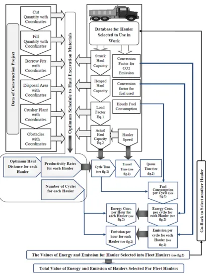
Figure 1. Structure of the model for estimating the energy usage and CO2 emissions of haulers used
in earthwork operations.
3.1. Collecting Input Data
of the excavated material is used to calculate a load factor (Lf) for the hauler (see Equation (1)), which is used to compute the actual hauling capacity of each hauler in the second step.
% = (100%)
(100% + swell %) (1)
where: swell = swelling factor (%).
In addition, it is necessary to compile the hauler database, which records information on the struck and heaped capacity, maximum speed, load factor, and hourly fuel consumption for each hauler selected for inclusion in the assessment (see Figure 1). These data are complemented with the estimated actual hauling capacity of each hauler (Hcact(LCM/cycle)) (i.e., LCM = Loose Cubic Meters), which is computed from their heaped capacity and the load factor using Equation (2):
[LCM/cycle] = ∗ (%) (2)
where: Hc= Heaped haul capacity, Lf = Load factor (%). 3.2. Generating a Schedule
The second step in the modeling process involves generating an optimum schedule using input data from the first stage. The optimum schedule is a plan designed mainly on the basis of the planners’ perspective and experiences, with the aim of maximizing the utilization of each hauler while ensuring that the requisite amounts of material are moved to and from each location. The hauler data are vital in the generation of the optimum plan because the final outputs of this stage are presented in terms of optimal haul distances, productivity [34], and cycle numbers (see Figure 1), all of which depend on the hauler data (i.e., capacity, speed, load factor, fuel type, and hourly fuel consumption) [48]. An average hauler speed (St (km/h)) is defined on the basis of the conditions and surface characteristics of the construction site, the terrain, the routes the haulers will travel, and the path conditions [44].
3.3. Assessing Energy Consumption and CO2 Emissions
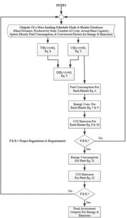
The third stage of the modeling process involves using a new algorithm to assess each hauler’s energy consumption and CO2 emissions (see Figure 2), based on previously obtained results and data (i.e., haul distance, productivity rate, number of cycles, actual haul capacity, speed, hourly fuel consumption, conversion factors for energy & emission). To begin with, it is necessary to compute a cycle time for each hauler (Ct(h/cycle)) that depends on the actual haul capacity (Hcact (LCM/cycle)) and the production rate (Pr (LCM/h)), as shown in Equation (3):
[h/cycle] = (3)
where: Hcact = Actual haul capacity, Pr = Production rate.
It is also necessary to calculate the travel time (Tt) for each hauler, i.e., the time required to haul and return, Hd (km/cycle); see Equation (4). This quantity is used to compute the estimated queue time (Qt) for each hauler in each cycle, which depends on the cycle time and travel time (see Figure 2) as well as the loading time (Lt) and dumping time (Dt) which depend on the properties of the hauler and loading server [49] (see Equation (5)).
[ℎ/ ] = 2 ∗ (4)
where: St = Hauler speed, Hd = Haul distance.
[ℎ/ ] = [ − ( + + )] (5)
where: Ct = Cycle time, Lt = Loading time, Dt = Dumping time, Tt = Travel time.
[L/cycle] = ∗ (6)
where: Fc = Fuel consumption per hour, Ct = Cycle time.
The energy consumption for each hauler per cycle (Ec (MJ/cycle)) can be calculated using the hauler’s fuel consumption per cycle, which is obtained as described above (see Figure 2) and the energy conversion factor (Ef (MJ/L)) for the fuel type that the hauler uses, as shown in Equation (7).
[MJ/cycle] = ∗ (7)
where: Fc = Fuel consumption per cycle, Ef = Energy conversion factor.
Similarly (see Figure 2), each hauler’s CO2 emissions per cycle (CO2E (kg/cycle)) can be calculated from its fuel consumption per cycle and the conversion factors for CO2 emission (Cf (kg/L)) (see Equation (8)).
[kg/cycle] = ∗ (8)
where: Fc = Fuel consumption per cycle, Cf = CO2 emissions conversion factor.
The estimated energy consumption (Ech (MJ/h)) and CO2 emissions (CO2Eh (kg/h)) per hour of hauler work on earthwork activities can be estimated from the number of cycles (Nc (cycle/h)) per hour for each hauler based on the optimum hauling schedule (see Equations (9) and (10)).
[MJ/h] = ∗ (9)
where: Ec = Energy consumption per cycle, Nc = Number of cycles per hour.
[kg/h] = ∗ (10)
where: CO2Eh = CO2 emission per cycle, Nc = Number of cycles per hour.
Having performed all of these calculations, their results can be compared to the regulations and requirements that apply to the project (see Figure 2) in order to determine which (if any) of the initially considered haulers should be selected. If none of the haulers satisfy all of the criteria, one can resume the process from the end of the first stage (the creation of the optimum schedule) and examine alternative haulers. Once a hauler that satisfies the project’s energy consumption and CO2 emission requirements has been identified (see Figure 2) each of the other haulers called for by the optimum schedule is evaluated similarly until all of the hauling requirements have been met.
Once the energy consumption and CO2 emissions of each individual hauler have been predicted, they can be combined to obtain total energy consumption (Echt) and CO2 emission (CO2Eht) values for the full set of haulers that will constitute the hauling fleet for the project. These quantities will depend on the number of each hauler type required under the optimum plan (see Figure 2) and are computed using Equations (11) and (12). These whole-fleet values can once again be compared to the project requirements to determine whether the proposed plan can be accepted (see Figure 2).
[MJ/h] = (11)
where: n = number of haulers; i = 1, 2, 3, …, n.
[kg/h] = (12)
where: n = number of haulers; i = 1, 2, 3, …, n.
4. Application of the Proposed Model in a Case Study
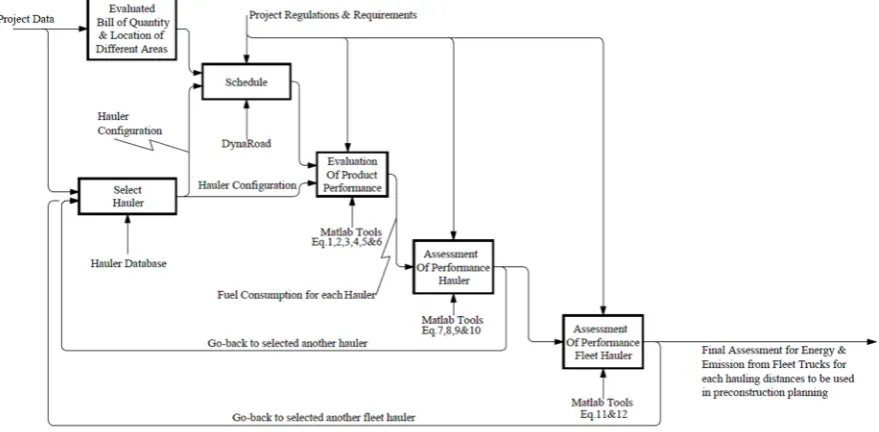
To evaluate its performance, the proposed model was tested in a case study. Figure 3 presents an Integrated Definition for Function Modeling (IDEFO) representation of a streamlined process for estimating energy consumption and emissions in earthwork operations. The generic procedure for applying the detailed model will be outlined below, along with a brief discussion of the project that was selected to test and demonstrate the model.
Data were collected from a new road construction project (väg 870) in Kiruna municipality, northern Sweden. The case study data were obtained from the project documentation and consisted of the project tender, which provides exact bills of quantities for earthwork activities and operations in addition to information on the size and location of borrow pits, disposal areas, and other relevant project-related information. The planned road had two lanes with a maximum design speed of 80 km/h and a width of 7.5–9 meters. It was designed to bear heavy traffic to and from a facility operated by the company LKAB and also to serve tourists and public traffic to and from Nikkaluokta.
load (i.e., the volume of material carrying above the body sides) [51]. Hence use the heaped capacity as a designed capacity for trucks. Moreover, the trucks were assumed to travel at a constant 50 km/h and brake effects were neglected. It was further assumed that all of the haulers worked with a single server (excavator), whose energy consumption and emissions were not included in those of the fleet. The swell factor of the excavated material was assumed to be 30%, giving a load factor of 0.769. The energy conversion factor and CO2 emission conversion factor for diesel engines were set to Ef= 36.0 MJ/L [52] and Cf= 2.614 kg/L, respectively [53].
Two computer programs were used to create a detailed model in the case study: DynaRoad is ‘Project management software for heavy civil engineering projects. It is used for planning and optimizing the mass-haul of an earthworks project based on the location of materials. It helps in creating a construction schedule and monitoring the progress of the project’ [54]. It was used to draw up the optimal schedule for earthwork operations [55,56], and Matlab was used to solve the necessary equations and determine the relationships between the model’s parameters (see Figure 3) so as to estimate the energy consumption and emissions.
The road construction data were entered into an Excel file, taking care to ensure consistency of units, in order to avoid errors during processing with DynaRoad in the first stage of the model building process [57]. The bill of quantities was then imported into DynaRoad along with the hauler database to enable the generation of a schedule based on the project’s activities, including all necessary resource adjustments. Data from the DynaRoad resource report and optimum schedule such as the haul distance, productivity rate, and number of rotations were exported into an Excel file containing data from the hauler database including information on the haulers’ actual haul capacity, speed, hourly fuel consumption, and conversion factors for energy & emissions. Matlab is then used to solve Equations (1)–(12) with the data from the Excel file. The resulting output can be tuned by the planner so that only the parameters of interest are displayed. In addition, the planner can go back to earlier stages of the modeling process in order to ensure that the solutions obtained comply with the applicable project regulations. For example, the estimated energy consumption and CO2 emissions for either individual hauler types or the fleet as a whole can be compared to the relevant environmental regulations and limitations in order to determine whether the evaluated configuration should be accepted or whether it is necessary to go back to the hauler database and evaluate alternative options (see Figure 3).
The planner can also vary the swell factor to determine how modifying the load factor affects the actual haul capacity, production rate, and cycle time, and thus the haulers’ queue times, which are computed during the third stage of the modeling process. Because the queue time strongly affects energy consumption and emissions (i.e., long queue times imply significant idle time; see queue time at Figures 1 and 2) [37], the selection of haulers might need to be modified. The final outputs of the modeling process include estimates of the hourly energy consumption and CO2 emissions for individual haulers and the fleet as a whole, enabling meaningful evaluation of the environmental impact of the planned earthwork operations.
The most important model outputs are the optimum haul distance, productivity rate, number of cycles, cycle time, queue time, fuel consumption based on cycle time, energy consumption per cycle and per hour, CO2 emissions per cycle and per hour, and the total hourly energy consumption and CO2 emissions for the selected hauler fleet. It should be noted that all of these values are estimated for each hauler and each haul distance. The maneuver time for each hauler is included in their loading times, and the reserve time is included in the queue time (see Table A1 in Appendix A).
5. Results & Discussion
Table A1 (Appendix A) shows the model’s predictions of the productivity, number of cycles, cycle time, queue time, energy consumption, and CO2 emissions for the three hauler models considered in the case study, over hauling distances ranging from 50 m to 23,000 m. These quantities were computed using equations 1 to 8 and the case study data. The results of the DynaRoad computations were verified to represent a mass optimized schedule [54,56,57] by performing a resource adjustment to achieve a zero surplus and zero deficit for the utilized resources based on the report on the hauling resources. The model’s output provided detail on several path-moving scenarios for haulers and included quantities relevant to planners during the preconstruction phase and construction managers during the construction phase. For example, it includes cycle times for each hauler model over a wide range of haulage distances, giving construction managers a clear understanding of the expected timing of earthwork activities that could be used for work monitoring during the execution phase to rapidly identify unexpected deviations from the schedule. The cycle time is also useful to planners because it directly affects the cost of hauling operations [14]. Consequently, it is important to consider when comparing different hauling options.
The model’s most important outputs are the predicted energy consumption and CO2 emissions of the haulers, which the planners and estimators need to know during the planning phase in order to devise a work plan that will satisfy the relevant environmental regulations. The model provides detailed information on the energy usage and cycle times of each hauler for a wide range of haulage distances. It therefore gives planners a clear overview of the energy consumption and environmental consequences of earth moving operations, allowing them to readily determine which individual haulers and fleet structures are most efficient or best able to satisfy the relevant environmental criteria.
Figure 4. (a) Energy consumption; and (b) CO2 emissions as functions of the haul distance for the
three hauler models considered in the case study.
The actual haul capacity, horsepower and hourly fuel consumption of hauler 773E were lower compared to hauler 775G. However, hauler 773E had higher energy consumed and CO2 emissions than hauler 775G even though this is not what would be expected given the difference in their haul capacities [48]. As shown in Table A1, the production rates for hauler 773E were substantially lower (see Figure 4a,b) than those for hauler 770G (i.e., it has a lower haul capacity) when the haulage distance exceeded 1 kilometer. In addition, hauler 773E had a longer cycle time than the other haulers. These contrasting trends in the productivity rate and cycle time for hauler 773E are due to the nature of its optimum work plan for mass haulers, which involves using paths and routes with multiple intersections linking several different construction facilities [45]. This reduced its productivity rates and increased its cycle time, leading to high energy and emissions, as well as higher queue times than were predicted for the other haulers. These outcomes are also reflected in the three haulers’ energy and emission curves (Figure 4a,b), which show that the energy consumption and emissions for hauler 773E increased sharply between haulage distances of 19–21 km but then decreased a little between 21 and 22 km before resuming steady growth.
The relationship between the haulers’ productivity rates and haul distances also highlighted the divergence of 773E: its productivity falls below that of hauler 770G at haul distances above 3 km (see Figure 5), suggesting that obstacles on the route selected for 773E affected its energy consumption and CO2 emissions.
Figure 5. The relationships between the productivity rates of the three haulers and the haul distance.
to determine whether the plan could be expected to satisfy the environmental regulations & conditions for the project (see Table 1).
Table 1. Hourly energy consumption and emissions for each individual hauler model and the whole fleet considered in the case study.
Item Caterpillar
770G
Caterpillar 773E
Caterpillar
775G Fleet
Energy consumption (MJ/h) 1153.799 1729.803 1943.995 4827.597
CO2 Emission (kg/h) 83.73 125.69 141.12 350.63
The final estimate of the fleet’s energy consumption was then used to identify an optimal hauling distance for the fleet’s operations (see Figure 6) given a targeted productivity rate and level of energy consumption.
Figure 6. Identifying an optimum fleet work plan that achieves acceptable productivity and energy consumption.
These results allow the planner to estimate the fleet’s energy consumption and CO2 emissions due to a given work duty, over a working day (involving multiple duties), over a working week, or over the complete duration of the project (assuming constant conditions and specifications; see example 1 below).
The modeling approach was used to predict the hourly energy consumption & CO2 emissions for three hauler models that were hauling material over a distance of 4 km in the case study discussed in Section 4. There were three particular quantities of interest:
I. The total energy consumption for each hauler per day if a working shift lasts for 8 h and there are two such shifts per work day.
II. The total CO2 emissions for each hauler per day under the above conditions.
III. The fleet’s total daily energy consumption & CO2 emissions under the above conditions.
Table 2. The energy consumption, CO2 emissions, and number of cycles for the three haulers
considered in the case study given a haul distance of 4 km.
Item Caterpillar 770G Caterpillar 773E Caterpillar 775G
Ec (MJ/cycle) 256.399 576.601 474.145
CO2E (kg/cycle) 18.62 41.87 34.43
Nc (cycle/h) 4.5 3.0 4.1
Haul distance (km) 4 4 4
Solution:
Where: Nh = Number of work hours per duty; Nd = Number of work duty per day (a) According to the data in table 3;
[ / ] = ∗ … … … ℎ
[ / ] = ∗ ∗ … … … … …
[ / ] = ∗ ∗ ∗ … … … …
[ / ] = 256.399 ∗ 4.5 ∗ 8 ∗ 2 = 18460.73 … … … … 770 [ / ] = 576.601 ∗ 3.0 ∗ 8 ∗ 2 = 27676.48 … … … … 773 [ / ] = 474.145 ∗ 4.1 ∗ 8 ∗ 2 = 31103.91 … … … … 775
(b) According to table 3 data;
[ /ℎ] = ∗ … … … ℎ
[ / ] = ∗ ∗ … … … … …
[ / ] = ∗ ∗ ∗ … … … …
[ / ] = 18.62 ∗ 4.5 ∗ 8 ∗ 2 = 1340.46 … … … 770 [ / ] = 41.87 ∗ 3.0 ∗ 8 ∗ 2 = 2009.65 … … … 773 [ / ] = 34.43 ∗ 4.1 ∗ 8 ∗ 2 = 2258.5 … … … 775
(c) Total daily fleet energy consumption and emissions:
[ / ] = 18460.73 + 27676.48 + 31103.91 = 77241.12 … … … ℎ ℎ
[ / ] = 1340.46 + 2009.65 + 2258.5 = 5608.61 … … … ℎ ℎ
The main limitation of the model presented is the assumption that all haulers in the fleet serve a single excavator. This could be addressed by extending the model to allow for multiple excavators and loaders. It would also be beneficial to evaluate the model’s performance by comparing its predictions to those of non-road & off-road models. In addition, the model could be refined to enable more systematic evaluation of hauling fleet compositions in order to minimize energy consumption and emissions. Finally, it would be useful to incorporate additional predictive factors into the model, such as the age of the hauler’s engine, hauler speed, idle time, and loading and dumping times.
6. Conclusions
This paper presents a detailed model for estimating the embodied energy and CO2 emissions due to mass hauling operations in road construction. The model used a mass optimized construction plan in the case study together with a developed algorithm and manufacturers hauler data to estimate quantities relevant to planners, such as the haul distance, productivity rate, and number of cycles. These data can be combined and sorted into groups for later use when planning similar earth-moving operations.
(kg/cycle or hour). The model was applied in a case study on a real-world construction project, demonstrating its ability to predict haulers’ fuel consumption, emissions, and productivity. Overall, the results presented herein demonstrate that the new modeling approach is powerful and flexible, and should be useful to planners needing to predict the emissions and energy consumption of mass haulers in future road construction projects.
The model presented here will be extended to include other pollutant sources, such as carbon monoxide, hydrocarbons and nitrogen oxides. The comparison of the present model with other methods in terms of the degree of improvement will be a key research area in the future investigation.
Author Contributions: The different knowledge and experience of each author has equally contributed to the development and final version of the article. As the main author, Hassanean Jassim wrote and compiled most of this paper. Also, the proposed model and application wrote and performed by Hassanean Jassim. Weizhuo Lu suggested and reviewed many ideas on the paper to support work. Thomas Olofsson supervised and reviewed the work throughout the study. Finally, all authors were involved in all steps of this study.
Appendix A
Table A1. The model’s output for the three haulers included in the case study.
Terms Productivity Rate (LCM/h) Number of Cycles (Cycle/h) Cycle Time (h/Cycle) Queue Time (h/Cycle)
Haul Distance
(m) 770G 773E 775G 770G 773E 775G 770G 773E 775G 770G 773E 775G
50 187.1 386.1 464.8 9.85 14.3 14.52 0.1015 0.0699 0.0688 Nil Nil Nil
100 184.3 368.1 450.4 9.7 13.63 14.08 0.1031 0.0733 0.0710 Nil Nil Nil
250 176.7 324.0 411.2 9.3 12.0 12.850 0.1075 0.0833 0.0778 Nil Nil Nil
500 164.3 270.0 360.0 8.65 10.0 11.250 0.1156 0.1 0.0889 Nil Nil Nil
1000 145.3 202.5 288.0 7.65 7.5 9.0 0.1308 0.1333 0.1111 Nil Nil Nil
2000 117.8 135.0 205.6 6.2 5.0 6.42 0.1613 0.20 0.1556 Nil 0.0200 Nil
3000 98.8 101.7 160.0 5.20 3.77 5.0 0.1923 0.2655 0.200 Nil 0.0455 Nil
4000 85.5 81.0 131.2 4.5 3.0 4.1 0.2222 0.3333 0.2439 Nil 0.0733 Nil
5000 75.0 67.5 110.4 3.95 2.5 3.45 0.2533 0.4000 0.2899 Nil 0.1000 Nil
6000 66.5 57.6 96.0 3.5 2.13 3.0 0.2857 0.4688 0.3333 Nil 0.1288 Nil
7000 59.8 50.4 84.8 3.15 1.87 2.65 0.3177 0.5357 0.3774 Nil 0.1557 Nil
8000 55.1 45.0 76.0 2.9 1.67 2.38 0.3448 0.6000 0.4211 Nil 0.1800 0.0011
9000 50.3 40.5 68.8 2.65 1.5 2.15 0.3777 0.6667 0.4651 Nil 0.2067 0.0051
10000 46.6 36.9 62.4 2.45 1.37 1.95 0.4077 0.7317 0.5128 Nil 0.2317 0.0128
11000 43.7 34.2 57.6 2.3 1.27 1.8 0.4348 0.7895 0.5556 Nil 0.2495 0.0156
12000 40.8 31.5 53.6 2.15 1.17 1.67 0.4657 0.8571 0.5970 Nil 0.2771 0.0170
13000 38.0 28.8 49.6 2.0 1.07 1.55 0.5 0.9375 0.6452 Nil 0.3175 0.0252
14000 36.1 27.0 46.4 1.9 1.0 1.45 0.5263 1.0000 0.6897 Nil 0.3400 0.0297
15000 34.2 25.2 44.0 1.8 0.93 1.38 0.5556 1.0714 0.7273 Nil 0.3714 0.0273
16000 32.3 23.4 40.8 1.7 0.87 1.2800 0.5882 1.1538 0.7843 Nil 0.4138 0.0443
17000 30.4 22.5 39.2 1.6 0.83 1.23 0.625 1.2 0.8163 Nil 0.4200 0.0363
18000 29.4 21.6 36.8 1.55 0.8 1.15 0.6463 1.2500 0.8696 Nil 0.4300 0.0496
19000 27.5 20.7 35.2 1.45 0.77 1.1 0.6909 1.3043 0.9091 Nil 0.4443 0.0491
20000 26.6 18.9 33.6 1.4 0.7 1.05 0.7143 1.4286 0.9524 Nil 0.5286 0.0524
21000 25.7 18.0 32.0 1.35 0.67 1.0 0.7393 1.5 1.0 Nil 0.5600 0.0600
22000 24.7 18.0 30.4 1.3 0.67 0.95 0.7692 1.5 1.0526 Nil 0.5200 0.0726
23000 23.8 17.1 28.8 1.25 0.63 0.9 0.7983 1.5789 1.1111 Nil 0.5589 0.0911
Terms Energy Consumption (MJ/Cycle) Energy Consumption (MJ/h) CO2Emission (Kg/Cycle) CO2Emission (Kg/h)
Haul Distance
(m) 770G 773E 775G 770G 773E 775G 770G 773E 775G 770G 773E 775G
50 117.1692 120.9636 133.8372 1154.11662 1729.7795 1943.3161 8.5077 8.7834 9.7181 83.80084 125.6026 141.1068
100 118.9483 126.8802 138.1172 1153.7987 1729.3771 1944.6907 8.6370 9.2129 10.0288 83.7789 125.5718 141.2055
250 124.0632 144.1512 151.2828 1153.7878 1729.81440 1943.9840 9.0085 10.467 10.985 83.7790 125.604 141.157
500 133.4268 172.98 172.8 1134.1278 1729.8000 1944.0000 9.6883 12.560 12.547 82.350 125.6 141.15
1000 150.8753 230.64012 216.0000 1154.1959 1729.8009 1944.0000 10.9552 16.7470 15.6840 83.80728 125.6025 141.156
Peer-reviewed version available at
Energies
2016
,
9
, 802;
2000 186.0966 345.9600 302.5681 1153.7989 1729.8000 1942.4873 13.5127 25.1205 21.9698 83.77874 125.6025 141.0461 3000 221.8860 459.2160 388.8000 1153.8072 1731.2443 1944.0000 16.111 33.346 28.231 83.777 125.71 141.15 4000 256.3999 576.6012 474.1452 1153.7996 1729.8036 1943.9953 18.6175 41.8676 34.4283 83.7787 125.602 141.156 5000 292.2959 691.9200 563.4781 1154.5687 1729.8000 1943.9995 21.2239 50.2411 40.9148 83.83440 125.6027 141.1560 6000 329.6570 810.8438 648.0000 1153.7996 1727.0974 1944.0000 23.9368 58.8763 47.052 83.7788 125.4065 141.156 7000 366.5920 926.6785 733.5850 1154.7647 1732.8888 1944.0001 26.6187 67.2872 53.2664 83.84890 125.8270 141.1559 8000 397.86192 1037.880 818.52624 1153.7996 1733.2596 1948.0925 28.8892 75.3616 59.4341 83.77868 125.8538 141.4531 9000 435.8304 1153.1988 904.1868 1154.95056 1729.79820 1944.0016 31.6460 83.7351 65.6540 83.8619 125.6026 141.1561 10000 470.4336 1265.7074 996.9232 1152.5623 1734.019 1944.0002 34.1587 91.9044 72.3877 83.68881 125.9090 141.1560 11000 501.6521 1365.6316 1080 1153.7998 1734.3521 1944.0000 36.4255 99.1600 78.4200 83.77865 125.9332 141.156 12000 537.3090 1482.6856 1160.5972 1155.21435 1734.7421 1938.1973 39.0146 107.6595 84.272 83.88139 125.9616 140.7342 13000 576.9 1621.6877 1254.1932 1153.8000 1735.2058 1943.9995 41.8893 117.753 91.068 83.7786 125.9957 141.1554 14000 607.26312 1729.800 1340.6897 1153.7999 1729.8000 1944.0000 44.0941 125.6027 97.3490 83.77879 125.6027 141.15605 15000 641.00016 1853.3570 1413.8183 1153.8003 1723.6221 1951.0692 46.5437 134.5743 102.6589 83.77866 125.15409 141.66928 16000 678.7044 1995.9228 1524.7044 1153.7975 1736.4528 1951.6216 49.2816 144.926 110.711 83.7787 126.085 141.710 17000 721.125 2075.76 1586.9387 1153.8000 1722.8808 1951.9346 52.3617 150.7232 115.2294 83.77872 125.1002 141.7321 18000 745.6644 2162.25 1690.434 1155.7798 1729.8000 1943.9991 54.1427 157.003 122.744 83.92118 125.6024 141.1556 19000 797.1710 2256.2608 1767.2728 1155.8980 1737.3208 1944.0000 57.8835 163.8296 128.3236 83.931075 126.14879 141.15596 20000 824.1430 2471.1430 1851.4285 1153.8001 1729.8001 1943.9999 59.8419 179.4324 134.4343 83.77866 125.6026 141.1560 21000 853.0056 2594.700 1944.000 1151.5576 1738.4490 1944.0000 61.9376 188.404 141.156 83.6157 126.230 141.156 22000 887.5404 2594.700 2046.316 1153.8025 1738.4490 1943.9998 64.4452 188.404 148.585 83.7787 126.230 141.155 23000 921.1007 2731.2631 2160.000 1151.3759 1720.6958 1944.0000 66.8822 198.3201 156.840 83.60275 124.9416 141.156
Peer-reviewed version available at
Energies
2016
,
9
, 802;
1. Hajji, A.M.; Lewis, M.P. Development of Productivity-based Estimating Tool for Fuel Use and Emissions from Earthwork Construction Activities. J. Constr. Eng. Proj. Manag. 2013, 3, 58–65.
2. Ahn, C.; Lee, S.; Peña-Mora, F.; Abourizk, S. Toward Environmentally Sustainable Construction Processes: The U.S. and Canada’s Perspective on Energy Consumption and GHG/CAP Emissions. Sustainability 2010, 2, 354–370.
3. Zeng, Y.; Cai, Y.; Huang, G.; Dai, J. A Review on Optimization Modeling of Energy Systems Planning and GHG Emission Mitigation under Uncertainty. Energies 2011, 4, 1624–1656.
4. Chen, Y.; Liu, B.; Shen, Y.; Wang, X. The energy efficiency of China’s regional construction industry based on the three-stage DEA model and the DEA-DA model. KSCE J. Civ. Eng. 2016, 20, 34–47.
5. Lewis, P.; Rasdorf, W.; Frey, H.C.; Pang, S.; Kim, K.; Requirements and incentives for reducing construction vehicle emissions and comparison of nonroad diesel engine emissions data sources. J. Constr. Eng. Manag. 2009, 135, 341–351.
6. Chow, J.C. Diesel engines: Environmental impact and control. J. Air Waste Manag. Assoc. 2001, 51, 1258– 1270.
7. Thompson, R.J.; Visser, A.T. Mine haul road maintenance management systems. J. S. Afr. Inst. Min. Metall. 2003, 103, 303–312.
8. Park, K.; Hwang, Y.; Seo, S.; Seo, H. Quantitative assessment of environmental impacts on life cycle of roads. J. Constr. Eng. Manag. 2003, 129, 25–31.
9. Li, H.; Lei, Z. Implementation of Discrete-Event Simulation (DES) in Estimating & Analyzing CO2 Emission
during Earthwork of Building Construction Engineering. In Proceedings of the International Conference on Industrial Engineering and Engineering Management, Xiamen, China, 29–31 October 2010; pp. 87–89. 10. Jang, W.; You, H.; Han, S.H. Quantitative Decision Making Model for Carbon Reduction in Road
Construction Projects Using Green Technologies. Sustainability 2015, 7, 11240–11259.
11. Hellström, E.; Ivarsson, M.; Åslund, J.; Nielsen, L. Look-ahead control for heavy trucks to minimize trip time and fuel consumption. J. Control Eng. Pract. 2009, 17, 245–254.
12. Kaboli, A.S.; Carmichael, D.G. Truck dispatching and minimum emissions earthmoving. J. Smart Sustain. Built Environ. 2014, 3, 170–186.
13. ICF Consulting. Emission Reduction Incentives for Off-Road Diesel Equipment Used in the Port and Construction Sectors; 2005.
14. Carmichael, D.G.; Lea, O.L.; Balatbat, M.C.A. Emissions Management of Urban Earthmoving Fleets. In Proceedings of the International Conference on Engineering, Project, and Production Management, Port Elizabeth, South Africa, 26–28 November 2014; pp. 262–271.
15. Peña-Mora, F.A.; Ahn, C.; Golparvar-Fard, M.; Hajibabai, L.; Shiftehfar, S.; An, S.; Aziz, Z.; Song, S. A Framework for Managing Emissions during Construction. In Proceedings of the NSF International Workshop on Green Buildings and Sustainable Construction, Cairo, Egypt, 2009.
16. Lewis, P.; Hajji, A. Estimating the Economic, Energy, and Environmental Impact of Earthwork Activities. In Proceedings of the 2012 Construction Research Congress, West Lafayette, IN, USA, 21–23 May 2012; ASCE: pp. 1770–1779.
17. Carmichael, D.; Williams, E.; Kaboli, A. Minimum Operational Emissions in Earthmoving. In Proceedings of the 2012 Construction Research Congress, West Lafayette, IN, USA, 21–23 May 2012; ASCE: pp. 1869– 1878.
18. Kaboli, A.S.; Carmichael, D.G. Emission and Cost Configurations in Earthmoving Operations. Organ. Technol. Manag. Constr. 2012, 4, 393–402.
19. The Swedish Transport Administration’s Efforts for Improving Energy Efficiency and for Climate Mitigation. Trafikverket. Publication No. 2012:152. Available online: https://online4.ineko.se/trafikverket/ Product/Detail/43997 (accessed on 9 December 2015).
20. Trani, M.L.; Bossi, B.; Gangolells, M.; Casals, M. Predicting fuel energy consumption during earthworks. J. Clean. Prod. 2016, 112, 3798–3809.
21. Ofori, G.; Gang, G.; Briffett, C. Implementing environmental management systems in construction: Lessons from quality systems. J. Build Environ. 2002, 37, 1397–1407.
23. Chen, Z.; Li, H. Environmental Management in Construction: A Quantitative Approach; Taylor & Francis Group: London, UK; New York, NY, USA, 2007; p. 3, p. 4 and p. 23.
24. Zhang, B.; Peng, S.; Xu, X.; Wang, L. Embodiment Analysis for Greenhouse Gas Emissions by Chinese Economy Based on Global Thermodynamic Potentials. Energies 2011, 4, 1897–1915.
25. Directive, N.N. 97/68/EC of the European Parliament and of the Council of 16 December 1997 on the Approximation of the Laws of the Member States Relating to Measures against the Emission of Gaseous and Particulate Pollutants from Internal Combustion Engines to be Installed in Non-Road Mobile Machinery, 1998. Available online: http://ec.europa.eu/environment/air/transport/non_road.htm.
26. U.S. Environmental Protection Agency (EPA). Recommendations for Reducing Emissions from the Legacy Diesel Fleet, Report from the Clean Air Act Advisory Committee; 2006. Available online: http://www.epa.gov/cleandiesel/documents/caaac-apr06.pdf (accessed on 10 April 2006).
27. Hajji, A.M.; Lewis, M.P. Development of Productivity-Based Estimating Tool for Energy and Air Emissions from Earthwork Construction Activities. J. Smart Sustain. Built Environ. 2013, 2, 84–100.
28. Ahn, C.; Pan, W.; Lee, S.; Pena-Mora, F. Enhanced estimation of air emissions from construction operations based on discrete-event simulation. In Proceedings of the International Conference on Computing in Civil and Building Engineering, Nottingham, UK, 30 June–2 July 2010; pp. 237–243.
29. Rasdorf, W.; Frey, H.C.; Lewis, P.; Kim, K.; Pang, S.; Abolhassani, S. Field Procedures for Real-World Measurements of Emissions from Diesel Construction Vehicles. J. Infrastruct. Syst. 2010, 16, 216–225. 30. Marshall, S.; Rasdorf, W.; Lewis, P.; Frey, H. Methodology for Estimating Emissions Inventories for
Commercial Building Projects. J. Archit. Eng. 2012, 18, 251–260.
31. Arocho, I.; Rasdorf, W.; Hummer, J. Methodology to Forecast the Emissions from Construction Equipment for a Transportation Construction Project. In Proceedings of the 2014 Construction Research Congress, Atlanta, Georgia, 19–21 May 2014; ASCE: pp. 554–563.
32. Ahn, C.; Rekapalli, P.V.; Martinez, J.C.; Peña-Mora, F.A. Sustainability Analysis of Earthmoving Operation. In Proceedings of the Winter Simulation Conference, Austin, TX, USA, 13–16 December 2009; pp. 2605– 2611.
33. Martinez, J.C.; Ioannou, P.G. General purpose systems for effective construction simulation. J. Constr. Eng. Manag. 1999, 125, 265–276.
34. Kim, B.; Lee, H.; Park, H.; Kim, H. Greenhouse Gas Emissions from Onsite Equipment Usage in Road Construction. J. Constr. Eng. Manag. 2012, 138, 982–990.
35. Guggemos, A.A.; Horvath, A. Decision-Support Tool for Assessing the Environmental Effects of Constructing Commercial Buildings. J. Archit. Eng. 2006, 12, 187–195.
36. Ercelebi, S.G.; Bascetin, A. Optimization of shovel-truck system for surface mining. J. S. Afr. Inst. Min. Metall. 2009, 109, 433–439.
37. Akhavian, R.; Behzadan, A.H. Simulation-Based Evaluation of Fuel Consumption in Heavy Construction Projects by Monitoring Equipment Idle Times. In Proceedings of the Winter Simulation Conference, Washington, DC, USA, 8–11 December, 2013; pp. 3098–8108.
38. Kean, A.J.; Sawyer, R.F.; Harley, R.A. A Fuel-Based Assessment of off-Road Diesel Engine Emissions. J. Air Waste Manag. Assoc. 2000, 50, 1929–1939.
39. Frey, H.; Rasdorf, W.; Lewis, P. Results of a Comprehensive Field Study of Fuel Use and Emissions of Nonroad Diesel Construction Equipment. Transp. Res. Rec. J. Transp. Res. Board 2010, 69–76.
40. Hwang, H.; Davis, S. Off-Highway Gasoline Consumption Estimation Models Used in the Federal Highway Administration Attribution and Process. Center for Transportation Analysis Energy and Transportation Science Division; Oak Ridge National Laboratory; U.S. Department Of Energy: 2009. DE-AC05-00OR22725, ORNL/TM-2009/222.
41. Lucas, A.; Silva, C.A.; Neto, R.C. Life cycle analysis of energy supply infrastructure for conventional and electric vehicles. J. Energy Policy 2012, 41, 537–547.
42. Schwarzkopf, A.B.; Leipnik, R.B. Control of highway vehicles for minimum fuel consumption over varying terrain. J. Transp. Res. 1977, 11, 279–286.
43. Choi, Y.; Nieto, A. Optimal haulage routing of off-road dump trucks in construction and mining sites using Google Earth and a modified least-cost path algorithm. J. Autom. Constr. 2011, 20, 982–997.
45. Choi, Y.; Park, H.; Sunwoo, C.; Clarke, K.C. Multi-criteria evaluation and least-cost path analysis for optimal haulage routing of dump trucks in large scale open-pit mines. Int. J. Geogr. Inf. Sci. 2009, 23, 1541– 1567.
46. Larsson, S. Commercial vehicles, fuel efficiency and CO2 Challenges & Possible solutions. In Proceedings
of the IEA Freight Truck Fuel Economy Workshop Challenge Bibendum, Berlin, Germany, 20–21 May 2011; ACEA, Euro. Autom. Manuf. Assoc. Available online: www.iea.org/workshop/work/hdv/larsson.pdf (accessed on 11 November 2015).
47. O’Reilly, D.J.; Nichols, M.W.; Chu, S. Advancing Technology for America’s Transportation Future. An Oil and Natural Gas Advisory Committee to the Secretary of Energy, National Petroleum Council, U.S. Department of Energy, 2012. Available online: www.npc.org/reports/trans-future_fuels_summary-2012-lowres.pdf (accessed on 7 November 2015).
48. Kecojevic, V.; Komljenovic, D. Haul truck fuel consumption and CO2 emission under various engine load
conditions. Official Publication in SME. Mın. Eng. 2010, 62, 44–48.
49. Burt, C. An Optimisation Approach to Materials Handling in Surface Mines. Ph.D. Thesis, Curtin University of Technology, Bentley, Australia, 2008.
50. Caterpillar Performance Handbook, 42th ed.; Caterpillar Inc.: Peoria, IL, USA, 2012. Available online:
http://www.cashmanequipment.com/UserFiles/PDF/CaterpillarPerformance Handbook42.pdf (accessed on 15 April 2015).
51. Hagenbuch, L.G. Adapting the Off-Highway Truck Body Volumetric Process to Real World Conditions; SAE Technical Paper; 2000.
52. Clean Fleets Guide. Procuring Clean and Efficient Road Vehicles; International Council for Local Environmental Initiatives (ICLEI-Europe) Local Governments for Sustainability: Germany, 2014. Available online: http://www.clean-fleets.eu/ (accessed on 3 September 2016).
53. BIOMASS Energy Center. Carbon Emissions of Different Fuels. Fuels for Heating, Power and Transport. Available online: http://www.biomassenergycentre.org.uk/portal/page?pageid=75,163182&dad=portal &schema=PORTAL(accessed on 13 May 2015).
54. Kenley, R.; Harfield, T.; Pirzadeh, P. Mass-Haul Environmental Impact Minimisation. A Practical Method for Greening Road Procurement; Industry Report; Sustainable Built Environment National Research Centre (SBEnrc): 2012.
55. Kenley, R.; Harfield, T. Greening procurement of infrastructure construction: Optimizing mass haul operation to reduce greenhouse gas emissions. In Proceedings of the CIB W78eW102 International Conference, Sophia Antipolis, France, 26–28 October 2011.
56. Törnroos, N. Location-Based Planning as a Production Optimization Technique in Linear Heavy Construction. Master’s Thesis, Property Management Economics and Technology, Aalto University, Espoo, Finland, 24 November 2014.
57. DynaRoad 5.3. Scheduling, Production Control and Earthworks Management, User Manual, Topcon Part Number 1003961-01 Manual, DynaRoad, 2014. Available online: http://www.dynaroad.fi/pages /index.php?option=comcontent&task=view&id=69&Itemid=25&lang=en (accessed on 7 April 2015).