Quantile regression for overdispersed count data: a hierarchical method

(1)

R E S E A R C H

Open Access

Quantile regression for overdispersed count

data: a hierarchical method

Peter Congdon

Correspondence:

[email protected]

Queen Mary University of London, London, UK

Abstract

Generalized Poisson regression is commonly applied to overdispersed count data, and focused on modelling the conditional mean of the response. However, conditional mean regression models may be sensitive to response outliers and provide no information on other conditional distribution features of the response. We consider instead a hierarchical approach to quantile regression of overdispersed count data. This approach has the benefits of effective outlier detection and robust estimation in the presence of outliers, and in health applications, that quantile estimates can reflect risk factors. The technique is first illustrated with simulated overdispersed counts subject to contamination, such that estimates from conditional mean regression are adversely affected. A real application involves ambulatory care sensitive emergency admissions across 7518 English patient general practitioner (GP) practices. Predictors are GP practice deprivation, patient satisfaction with care and opening hours, and region. Impacts of deprivation are particularly important in policy terms as indicating effectiveness of efforts to reduce inequalities in care sensitive admissions. Hierarchical quantile count regression is used to develop profiles of central and extreme quantiles according to specified predictor combinations. Keywords:Quantile regression, Overdispersion, Poisson, Count data, Ambulatory sensitive, Median regression, Deprivation, Outliers

1. Background

Extensions of Poisson regression are commonly applied to overdispersed count data, focused on modelling the conditional mean of the response. However, conditional mean regression models may be sensitive to response outliers. We consider instead a Bayesian hierarchical approach to quantile regression of overdispersed count data, based on a Poisson log-normal (PLN) approach to overdispersion. The method set out here is for quantile regression for latent outcomes at the second stage of a hierarchical model. Focussing on median regression in particular, this method provides an approach to Bayesian robust regression for overdispersed count data.

The technique is first illustrated with simulated overdispersed counts subject to contam-ination, such that conditional mean regression is adversely affected. It is shown that the hierarchical median regression via a Poisson log-normal representation (HQRPLN) more accurately reproduces the regression parameters assumed in the simulation than negative binomial or standard PLN regression. The HQRPLN estimates for contaminated data are competitive with those of classical methods for robust regression using a negative binomial

(2)

density and M-estimation (Aeberhard et al. 2014; Chambers et al. 2014), and also with clas-sical methods for median regression for count data (Machado and Santos Silva, 2005). It is also shown that HQRPLN accurately identifies the contaminated observations.

A real application involves counts of ambulatory care sensitive (ACS) emergency admissions in 2014–15 according to 7518 English patient general practitioner (GP) practice. Such admissions are potentially avoidable given effective care and are often used as an index of health performance (Caminal et al. 2004). Predictors are practice deprivation, patient satisfaction with care (general satisfaction and satisfaction with opening hours), and the practice region of location. Hierarchical quantile Poisson log-normal regression is used to assess the most important predictors, variation in predictor effects by quantile, and varying impacts of predictors by region.

The applied focus of the paper adopts a Bayesian strategy and uses a quantile regression approach that has, as one aspect, the benefit of robustness compared to conditional mean regression, which is demonstrated using simulated data. However, we also aim to demon-strate the utility of quantile regression in an analysis of a health performance index. To set the broader context, we consider classical methods for robust regression of overdis-persed count data in section 2, before considering quantile regression, using classical methods and in terms of Bayesian implementation (section 3). Section 4 considers the Poisson log-normal representation for quantile count regression. The remaining sections involve data analysis: a simulation analysis involving contaminated count data (section 5), and finally, the ACS admissions analysis and results applying the HQRPLN method (sections 6 and 7).

2. Robust count regression via M-estimation and Bayesian strategies

Classical approaches to robust regression for data {yi, i = 1,.., n} on covariates Xi of

dimension p focus either on M-estimation, or median quantile regression (see next section). For linear regression under M-estimation, robustness may be achieved by incorporation in the estimation of objective functions Q(r) (Andersen, 2008) that downweight large positive and large negative standardized residuals ri= (yi−Xiβ)/s,

where β is a regression parameter, and s is a scale estimate. For linear regression,

estimation involves minimisation of Pn i¼1

Q rð Þi , with corresponding estimation equations

1 n

Pn i¼1

Xijψð Þ ¼ri 0, whereψ(r) =∂Q(r)/∂r is the score or influence function.

Regarding M-estimation for overdispersed counts, consider in particular, negative binomial NB(μi,σ) regression with offsets Oi, means μi= Oiexp(Xiβ), overdispersion

parameter σ, and the NB2 parameterisation (Aeberhard et al., 2014; Hilbe, 2011). Then robustness may be achieved by objective functions that downweight large positive and large negative residuals ri= (yi−μi)/V0.5(μi).

Thus Chambers et al. (2014) consider M-estimation for overdispersed counts using a negative binomial model. They estimate β using the Huber score function (Huber, 1973) and estimating equations

1 n

X

i

Δðy_i;μ_iÞ ¼0;

(3)

Δðy_i;μ_iÞ ¼ψð Þri w Xð Þi μi

Xi

V0:5 _μ i

ð Þ−að Þβ;

where the weights w(X_{i) may be used to downweight leverage points (covariate} outliers), and a(β) is a correction factor ensuring Fisher consistency. The Huber score function uses a cutpoint k to define (absolute) extreme residuals, such as k = 2, with ψ(r) = max(−k, min(k, r)). Chambers et al. (2014) use a robust moment estimator for θ= 1/σ, whereas Aeberhard et al. (2014) use M-estimation in a form of weighted maximum likelihood, preferring this on efficiency grounds.

Bayesian regression methods intended as robust to outliers include ε−contamination priors (Moreno and Pericchi, 1993), modified likelihoods such as weighted likelihoods (Greco et al. 2008; Agostinelli and Greco, 2013), and localized regression (Wang and Blei, 2017). For overdispersed count regression, in particular, an ε−contamination approach might involve negative binomial or Poisson log-normal representations, and specify a main model and contamination model. The contamination model would be assumed to apply for a small subpopulation, with small prior probabilityε(e.g.ε= 0.1 orε= 0.05), and might involve an intercept or variance shift as compared to the main model.

3. Quantile regression: classical and Bayesian approaches

An alternative approach to robustness, and the focus of this paper, is provided by quantile regression. Thus generalized linear models for discrete responses typically involve conditional mean estimation using both known predictors, and random effects to represent unknown covariates or overdispersion. However, mean regression models may be sensitive to response outliers and provide no information on factors affecting other distributional points (e.g. upper and lower 5% quantiles) of the response.

By contrast, quantile regression estimates the relationship between the qth quantile Qy(q|X) of the response y and covariates X (Koenker and Hallock, 2001). Quantile

regression was originally developed for continuous responses as count responses do not have continuous quantiles. For q∈(0, 1) and continuous y, classical quantile

regression involves minimizing P n i¼1

ρq yi−Xiβq

, where ρq(u) = u(q−I(u≤0)). A special

case is provided by median regression, involving minimization of the absolute

devia-tions, P n i¼1

y_i−Xiβ

. This reduces the impact of outliers (influential observations) in the

response space, providing a better fit for the majority of observations.

Chambers et al. (2014) extend M-estimation to quantile regression, including count regression. For linear regression the estimating equations become

1 n

Xn i¼1

XijΔq

y_i−Xiβq

s

¼0;

where Δq e_s ¼2ψ e_s ½qI eð >0Þ þð1−qÞI eð ≤0Þ, and s is a scale estimator. For

overdis-persed count data, similarly define scaled residuals

riq¼ yi−Qqð ÞXi

=V0:5 _Q qð Þμi

;

where Qq(Xi) = Oiexp(Xiβq). Then the estimating equations for β are

1 n

P

iΔq yi;Qqð ÞXi

(4)

where

Δq yi;Qqð ÞXi

¼ψq riq w Xð Þi

Qqð ÞXi Xi

V0:5 Qqð ÞXi

−a β_q :

By contrast, Machado and Santos Silva (2005) propose quantile regression for count data based on adding uniform noise u to count responses y (i.e. jittering count re-sponses), giving z = y + u, and apply quantile regression of the form

QziðqjXiÞ ¼ηqi¼ exp Xiβq

:

As discussed by Yu and Moyeed (2001), a Bayesian approach to quantile regression for y continuous is obtained using an Asymmetric Laplace distribution (ALD), with density function

ALDðyjη_q;δq;qÞ ¼

qð1−qÞ δq

exp

b

−ρqðy−ηqÞ δq

c

:

This distribution can in turn be represented as a scale mixture of normals (Tsionas, 2003). For observations i = 1,.., n, and assuming yi~ ALD(ηqi,δq, q), one has

y_i¼η_qiþξqWqiþ

2Wqiδq

q 1ð −qÞ

0:5

uqi;

where ξq ¼q 1ð1ð−−2qqÞÞ, δq> 0 , Wqi~ Exp(δq), and uqi∼N(0, 1), and the regression term

ηqi=β0q+ Xiβq may be expanded to include random effects.

One potential issue with quantile regression, whether under classical or Bayesian esti-mation, is quantile crossing. Estimated conditional quantile functions may violate the monotonicity principle, with η_q

1i>ηq2i when q1< q2for some covariate combinations,

or random effect values if the regression termsηqiinclude random effects. One can

ex-plicitly impose the constraintsη_q

ji>ηqj−1i (Bondell et al. 2010) in simultaneous

estima-tion involving multiple quantile points, while Wu and Liu (2009) propose a sequential procedure ensuring that a regression at an additional quantile does not cross with pre-vious ones.

Assuming Bayesian inference, one possible criterion for assessing quantile crossing is whether the posterior mean ηqi follow the monotonicity constraint. A more exacting

criterion considers all MCMC samples. In MCMC sampling (under simultaneous esti-mation) a full exploration of the parameter space may generate occasional quantile crossing which can be monitored via monotonicity indicators mit= 1 if monotonicity is

maintained for observation i at iteration t. The relevant criterion for monotonicity would then require thatP_imit¼n for all iterations. Where departures from monoton-icity are not pronounced, one can impose monotonmonoton-icity constrained sampling by reject-ing any iterations t where P_imit<n, and basing inferences only on retained samples whereP_imit¼n.

4. Methods: hierarchical poisson log-normal

(5)

continuous outcomes in the case of binary regression (Benoit and Van den Poel, 2012). In this paper, we follow a similar principle in an approach to quantile regression for overdispersed count data, avoiding the need for jittering.

This approach involves a scale mixture version of the ALD (Yu and Moyeed, 2001) within a hierarchical Poisson-lognormal representation to account for overdispersion (e.g. Connolly & Thibaut, 2012). The quantile regression is for latent outcomes at the second stage of the hierarchical model, focussed on estimating latent incidence rates or relative risks. The Poisson log-normal representation is per se advantageous in that the tails of the log-normal are heavier than for the gamma distribution, and for data with outliers, the Poisson log-normal model may give a better fit than the negative-binomial model (Connolly et al. 2009; Sohn 1994; Miranda-Moreno et al. 2005; Wang and Blei, 2017).

Thus for observed counts yi, one specifies for quantiles q = 1,.., Q,

y_i_ePoi μ_qi ; ð1Þ

μqi¼ exp νqi ;

νqieN β0qþXiβqþξqWqi;

2Wqiδq

q 1ð −qÞ

;

WqieExp δq :

The Wqi in (1) are measures of outlier status. Observations with higher Wqi have

higher variances (lower precisions) and hence diminished influence on the likelihood. Predictions for cases with high Wqiare likely to have a wide uncertainty interval. For

assessing which observations are response outliers in practice, the Wqithemselves may

be highly skewed, so measuring scale is problematic even using robust scale measures. However, outlier detection rules can be used, based on adjusted boxplot rules, which include the interquartile range as an implicit scale measure (Hubert and Vandervieren, 2008; Carling, 2000; Verardi and Vermandele, 2016). One may also monitor trans-formed Wqi (e.g. log or square root), namely Uqi= log(Wqi), or transformed ratios of

Wqito the exponential mean 1/δq, Uqi= log(Wqiδq), and consider thresholds in

standar-dised Uqifor detecting outliers.

Another option is to derive exceedance probabilities against the exponential mean, Pr(Wqi> 1/δq|Y), or based on pairwise comparison against other Wqj(j≠i), namely

1 n−1

P

j≠i Pr Wqi >WqjY

(Santos and Bolfarine, 2016), with higher exceedance

probabilities characterising observations disparate from the majority of observa-tions. The pairwise comparison measure can be obtained from monitoring ranks of sampled Wqi (e.g. using the rank command in rjags). Such exceedance probabilities

are analogous to those used in disease mapping applications to detect high relative disease risk (Richardson et al. 2004).

Santos and Bolfarine (2016) also mention outlier detection based on a Kullback-Liebler distance measure between estimated densities of each Wqi, though this

would be computationally intensive for large samples. A residual distance measure to detect outliers is mentioned by Benites et al. (2015), which for linear quantile

regression has the form dqi¼

yi−β0q−Xiβq

j j

δq . For the application here the equivalent

measure is dqi¼

νqi−β0q−Xiβq

j j

(6)

using graphical methods, but these become infeasible for large samples and instead one may consider standardised dqi to detect outliers.

If there are offsets Oi(expected counts, times or populations exposed, etc), then these

can be included as

y_i_ePoi μ_qi ; μqi¼Oiexp νqi ;

νqieN β0qþXiβqþξqWqi;

2Wqiδq

q 1ð −qÞ

:

In health applications, offsets are typically expected health events. In this case, ρqi= exp(β0q+ Xiβq) can be obtained as predicted relative risks specific to quantile.

If ∑yi=∑Oi then predicted relative risks will be centred around 1, and elevated

relative risks will be associated with a high probability that relative risks exceed 1, even at low quantiles.

Bayesian count regression often focuses on assessing cases with elevated mean inci-dence or mean relative risk. Under the quantile regression (1), extreme conditional quantiles of incidence (e.g. 5 and 95%) may be estimated from quantile specific regres-sion, which allows covariate impacts to vary by quantile. The ability to examine central and extreme quantiles in relation to particular covariate combinations may be import-ant for policy formulation or assessment (Reich et al. 2011). One may also focus on a lower quantile (such as 2.5 or 5%), and identify probabilities of excess incidence or rela-tive risk at this quantile. This type of issue may occur in other applications (e.g. finan-cial); for example, Takeuchi et al. (2006) mention that “For risk management and regulatory reporting purposes, a bank may need to estimate a lower bound on the changes in the value of its portfolio which will hold with high probability”.

5. Simulated data example

This analysis demonstrates that the HQRPLN method reproduces the underlying regression parameters for overdispersed count data subject to contamination, and also accurately identifies response outliers.

Data generation follows the approach set out by Aeberhard et al. (2014), which is concerned with robust estimation for negative binomial regression, except that a larger sample size of n = 10,000 is taken. Two predictors are assumed, X1, with values

gener-ated as standard normal, the other X2as binary (=1 for half the sample, = 0 for other

cases). Then with generating (“true”) regression parametersβ= (0.5, 0.8,−0.4), negative binomial means μ= exp(β0+β1X1+β2X2), and overdispersion parameter σ= 0.7, the

counts are generated in R as y < − rnbinom(n = n, mu = mu, size = 1/sigma). The mean count so generated is 1.9. The large sample size ensures that the regression parameters for the actual sample data are close to those used to generate the data, whereas for a smaller sample size (n = 200) the parameters for the sampled datasets fluctuate much more widely around the true values; this may be verified graphically using the R code (and negative binomial regression) in Additional file 1.

(7)

observations out of the total sample). We consider six contamination settings, namely C = 5, C = 10, C = 15, C = 20, C = 25 and C = 30. The R code is pro-vided in Additional file 1.

We compare Bayesian regression estimates for the contaminated samples according to (a) negative binomial regression; (b) a standard Poisson log-normal (i.e. conditional mean estimation); and (c) a median regression under the HQRPLN representation. Comparisons are included with the classical methods: the Aeberhard et al. (2014) method, using the glmrob.nb.r code from ttps://github.com/williamaeberhard/glmrob.nb; the Chambers et al. (2014) method, using the glm.mq.nb option in the R package CountMQ (note that this does not provide confidence intervals), and the Machados and Santos Silva (2005) method using lqm.counts (https://www.rdocumentation.org/packages/lqmm/versions/ 1.5.3/topics/lqm.counts).

Bayesian models are estimated using jagsUI in R. Normal priors with mean 0 and variance 1000 are assumed on regression parameters, and gamma priors, with shape 1 and inverse scale (rate) 0.001, are assumed on precision parameters and the HQRPLN parameter δ. Two chains are used, with convergence assessed using Brooks-Gelman-Rubin scale reduction factors (Brooks and Gelman, 1998).

Sensitivity to the prior onδmay be an issue. We consider, in addition to the gamma prior, a uniform prior onδ,δ~ U(0, 10000), and a parameterisation in terms of the ex-ponential mean rateϕ= 1/δ. Thus Wi~ exp(1/ϕ), log(ϕ) =ω0, withω0assigned a diffuse

normal N(0,1000) prior. It may be noted, in more general application terms, that the exponential rate prior potentially extends to a regression approach to explaining vari-ation in Wi, with observation specificϕi.

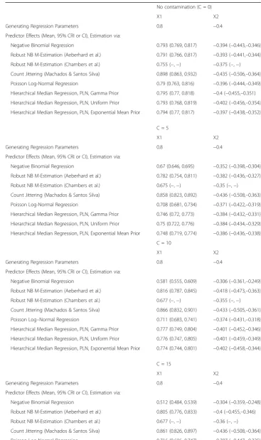
Table 1 contains the resulting regression parameter estimates. It can be seen that nega-tive binomial regression is most vitiated by response outliers, this distortion increasing with C. The Chambers et al. (2014) estimates are more robust than negative binomial re-gression, but not as robust as the Aeberhard et al. (2014) estimates or the HQRPLN esti-mates. Standard Poisson log-normal regression is more robust than the negative binomial regression and the Chambers et al. (2014) estimates, but outperformed by the HQRPLN method. The HQRPLN method provides estimates closer to the true values as compared to the Chambers et al. (2014) method, and the Machados and Santos Silva (2005) method, which tends to overestimateβ1. All credible intervals from hierarchical median PLN

re-gression include the true rere-gression parameter values except for β1under C = 5, and this

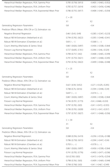
method is otherwise comparable to Aeberhard et al. (2014). Table 2 shows that posterior estimates ofδare very similar for different priors; there is no appreciable sensitivity.

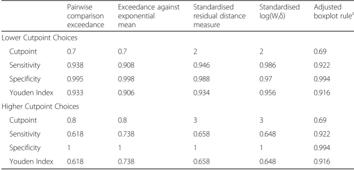
One advantage of the hierarchical median PLN regression is in outlier detection. This can be assessed in terms of the concordance between the contamination sample and ob-servations identified as having elevated Wi. In a real application, of course, the outliers

would not be known in advance. However, in the case of simulation we can evaluate clas-sification accuracy using established indices (Ruopp et al. 2008). We use five different out-lier detection methods, reporting their sensitivity, specificity and the corresponding Youden index (Ruopp et al. 2008): pairwise comparison exceedance rates (Santos and Bolfarine, 2016); exceedance rates against the exponential mean; a standardised version of the residual distance measure (Benites et al. 2015); standardised Ui= log(Wiδ); and the

modified boxplot rule (Hubert and Vandervieren, 2008) applied to posterior mean Wi.

(8)

Table 1Regression parameter estimates (Means and 95% CrI or 95% CI) by estimation method, contaminated and uncontaminated dataa

No contamination (C = 0)

X1 X2

Generating Regression Parameters 0.8 −0.4

Predictor Effects (Mean, 95% CRI or CI), Estimation via:

Negative Binomial Regression 0.793 (0.769, 0.817) ₋0.394 (₋0.443,_–0.346)

Robust NB M-Estimation (Aeberhard et al.) 0.791 (0.766, 0.817) ₋0.393 (₋0.441,_–0.344)

Robust NB M-Estimation (Chambers et al.) 0.755 (−,−) −0.375 (−,−)

Count Jittering (Machados & Santos Silva) 0.898 (0.863, 0.932) −0.435 (−0.506,–0.364)

Poisson Log-Normal Regression 0.79 (0.763, 0.816) ₋0.396 (₋0.444,_–0.349)

Hierarchical Median Regression, PLN, Gamma Prior 0.795 (0.77, 0.818) ₋0.4 (₋0.455,_–0.351)

Hierarchical Median Regression, PLN, Uniform Prior 0.793 (0.768, 0.819) −0.402 (−0.456,–0.354)

Hierarchical Median Regression, PLN, Exponential Mean Prior 0.794 (0.77, 0.817) −0.397 (−0.438,–0.352)

C = 5

X1 X2

Generating Regression Parameters 0.8 ₋0.4

Negative Binomial Regression 0.67 (0.646, 0.695) −0.352 (−0.398,–0.304)

Robust NB M-Estimation (Chambers et al.) 0.675 (₋,₋) ₋0.35 (₋,₋)

Poisson Log-Normal Regression 0.708 (0.681, 0.734) −0.371 (−0.422,–0.319)

Hierarchical Median Regression, PLN, Uniform Prior 0.75 (0.722, 0.776) ₋0.384 (₋0.434,_–0.329)

C = 10

X1 X2

Poisson Log–Normal Regression 0.711 (0.683, 0.741) −0.374 (−0.431,–0.318)

C = 15

X1 X2

Robust NB M-Estimation (Aeberhard et al.) 0.805 (0.776, 0.833) −0.4 (−0.455,–0.346)

(9)

The upper part of Table 3 sets out results if the threshold for exceedance rates is set at 0.7, and that for standardised measures set at 2. The latter threshold is a lower out-lier threshold for standardised measures mentioned by Wilcox (2016). Outout-lier detection Table 1Regression parameter estimates (Means and 95% CrI or 95% CI) by estimation method, contaminated and uncontaminated dataa(Continued)

Hierarchical Median Regression, PLN, Gamma Prior 0.785 (0.758, 0.813) −0.405 (−0.463,–0.352)

C = 20

X1 X2

C = 25

X1 X2

Count Jittering (Machados & Santos Silva) 0.861 (0.826, 0.897) ₋0.436 (₋0.508,_–0.364)

C = 30

X1 X2

Generating Regression Parameters 0.8 −0.4

Negative Binomial Regression 0.388 (0.356, 0.419) ₋0.256 (₋0.326,_–0.188)

Count Jittering (Machados & Santos Silva) 0.861 (0.826, 0.897) ₋0.436 (₋0.508,_–0.364)

Hierarchical Median Regression, PLN, Exponential Mean Prior 0.798 (0.768, 0.83) ₋0.41 (₋0.467,_–0.349) a

(10)

performance at these thresholds is slightly higher for the standardised Ui, with a 98.6%

sensitivity and 97% specificity. In general, setting outlier thresholds higher reduces sensitivity while raising specificity. Setting the exceedance probability threshold at 0.8, and the standardised measures threshold at 3 (Wilcox, 2016, page 45), reduces performance for the first four measures (Table 3, lower panel). The settings for the boxplot rule are unchanged, following Hubert and Vandervieren (2008) guidelines, and it now has better performance.

6. Case study application

The case study dataset consists of counts yi of ambulatory care sensitive (ACS)

emergency admissions for n = 7518 GP practices in England’s National Health Service (NHS) during 2014/15. The data are from the Care Quality Commission (source: https://www.cqc.org.uk/content/monitoring-gp-practices). The GP practices are ar-ranged into four regions, responsible for planning and commissioning health care. Unplanned emergency admissions, including those for care sensitive conditions rated as potentially avoidable or preventable (Tian et al. 2012), show wide socioeconomic inequalities, being higher from more deprived areas (Sheringham et al. 2016). However, effectiveness of NHS agencies in tackling these inequalities varies considerably. One way proposed to measure inequality is the slope index of the outcome on a measure of social deprivation (Regidor, 2004).

Table 2Estimatedδunder different priors and contamination levels

Contamination level Prior Mean Std devn 2.5% 50% 97.5%

C = 0 Gamma prior 3.48 0.07 3.35 3.48 3.62

Uniform prior 3.49 0.08 3.33 3.49 3.64

Exponential Mean Prior 3.50 0.07 3.36 3.49 3.65

C = 5 Gamma prior 2.97 0.05 2.87 2.97 3.07

Uniform prior 2.97 0.06 2.86 2.96 3.08

C = 10 Gamma prior 2.56 0.04 2.48 2.56 2.65

Uniform prior 2.57 0.04 2.49 2.56 2.64

C = 15 Gamma prior 2.39 0.04 2.31 2.39 2.47

Uniform prior 2.39 0.04 2.31 2.38 2.46

C = 20 Gamma prior 2.29 0.04 2.22 2.29 2.36

Uniform prior 2.28 0.04 2.21 2.28 2.36

C = 25 Gamma prior 2.21 0.04 2.15 2.21 2.29

Uniform prior 2.21 0.04 2.14 2.21 2.29

C = 30 Gamma prior 2.16 0.03 2.10 2.16 2.23

Uniform prior 2.16 0.04 2.10 2.16 2.24

(11)

The analysis here uses GP practices as the observational unit and considers impacts of deprivation on care sensitive emergency admissions, and regional differences in that impact. Predictors are a GP practice deprivation score, the Index of Multiple Deprivation or IMD (DCLG, 2015), and two measures of perceived access to care for each GP practice. Access to primary care has been shown to reduce emergency hospital attendances and admissions (Dolton and Pathania, 2016). The access indicators are from an annual survey of patent views regarding their primary care (the GP Patient Survey) and are proportions of patients ‘very satisfied’or ‘fairly satisfied’with their GP practice opening hours, and proportions of patients describing the overall experience of their GP surgery as fairly good or very good. These predictors are denoted IMD, SatHrs and OvExp for short. Two of these predictors are already on a [0,1] scale. In order that variations in the strength of impacts of predictors can be straightforwardly compared, the GP practice deprivation score (with a range from 3.2 to 66.5) is transformed to a

[0,1] scale using a linear transformation, _{max IMD}IMD_ð −min IMD_Þ₋_{min IMD}ð _ð Þ _Þ. A region indicator (regi) of

the GP practice location and affiliation is also included: 1 = London (reference), 2 = Midlands and East of England, 3 = North Of England, 4 = South of England (outside London).

The analysis involves Poisson lognormal regression, including the scale mixture ALD. Two models are compared. One assumes a common effect of deprivation on care sensi-tive emergencies. Thus let X1= IMD, X2= SatHrs, X3= OvExp, and Oidenote expected

admissions, based on England wide ACS rates by age. The first model assumes for quantiles q = 1,.., Q

νqieN ηqiþξqWqi;

2Wqiδq

q 1ð −qÞ

;

Table 3Outlier detection by different methods (C = 20) and different cutpoints

Pairwise comparison exceedance

Exceedance against exponential mean

Standardised residual distance measure

Standardised log(Wiδ)

Adjusted boxplot rulea

Lower Cutpoint Choices

Cutpoint 0.7 0.7 2 2 0.69

Sensitivity 0.938 0.908 0.946 0.986 0.922

Specificity 0.995 0.998 0.988 0.97 0.994

Youden Index 0.933 0.906 0.934 0.956 0.916

Higher Cutpoint Choices

Cutpoint 0.8 0.8 3 3 0.69

Sensitivity 0.618 0.738 0.658 0.648 0.922

Specificity 1 1 1 1 0.994

Youden Index 0.618 0.738 0.658 0.648 0.916

a

(12)

ηqi¼β0qþXi1β1qþXi2β2qþXi3β3qþI regð i¼2Þβ4qþI regð i¼3Þβ5q

þI regð _i¼4Þβ_6q:

The second model allows the impact of deprivation to vary by region. Thus

νqieN ηqiþξqWqi;

2Wqiδq

q 1ð −qÞ

;

ηqi¼β0qþXi1γiþXi2β2qþXi3β3qþI regð i¼2Þβ4qþI regð i¼3Þβ5q

þI regð _i¼4Þβ_6q;

γi¼β1qþI regð i¼2Þβ7qþI regð i¼3Þβ8qþI regð i¼4Þβ9q:

This model is relevant to assessing whether regions vary in their effectiveness in tack-ling inequality in ambulatory sensitive admission rates: higherγivalues indicate higher

socio-economically based inequalities in such admissions.

These models are compared using quantile regression over the 0.05, 0.50, and 0.95 (i.e. Q = 3) quantiles, with estimation simultaneous across the three quantiles. Regression analysis is carried out in WINBUGS14 (Lunn et al. 2000). Inferences are based on the second halves of 20,000 two chain runs with convergence assessed using Brooks-Gelman-Rubin diagnostics (Brooks and Gelman, 1998). Normal N (0,100) priors are adopted on βparameters, and gamma priors Ga (1,0.001) with shape 1 and rate 0.001 on scale parametersδq.

Model fit is assessed using the widely applicable information criterion (WAIC) (Watanabe, 2010). The WAIC involves two elements: a log pointwise predictive density (lpd) and a complexity estimate (pwaic), with the WAIC obtained as −2(lpd-pwaic). Posterior predictive model checks (Berkhof et al., 2000) are based on sampling replicate data yrep , q. First, predictive coverage is assessed by the proportion of observations

con-tained within the 95% credible intervals of yrep , qi(Gelfand, 1996). Second, denotingθas

model parameters, posterior predictive p-tests are obtained by evaluating specified test statistics, T(yrep , q|θ) and T(y|θ), and obtaining probabilities Pr[T(yrep , q|θ) > T(y|θ)]. The

test statistics are the likelihood ratio statistic P_iy_ilog y _i=μ_qi; the maximum yi; and the

total of y,P_iy_i.

7. Case study results

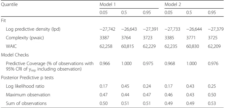
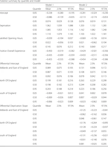
Table 4 shows an advantage in fit for the second model for two of the three quantiles, although posterior predictive checks for both are satisfactory. Table 5 shows the regres-sion parameters under the two models. Monotonicity is preserved using the more exacting criterion mentioned in section 3, namely thatP_imit¼n for all iterations.

(13)

comparable predictor levels, London and the South have lower levels of ambulatory sensitive admissions than the other two regions, with the North having the highest dif-ferential against London and the South.

Results for model 2 show show significantly lower differential slope effects at q = 0.05 for the Midlands, North and South regions (represented in parametersβ7q,β8q

and β9q). Table 6 shows the resulting overall deprivation slopes by region under model

2, with steepest slopes in London at q = 0.05, and in the South and Midlands at q = 0.95, and generally shallower slopes in the North.

There are different ways to represent the impacts of parameter estimates on estimated risks of ambulatory sensitive emergencies, and identifying priorities for intervention. One can demonstrate how relative risks vary by deprivation category and region, since differences in the slope index by region (as identified in model 2) imply varying gradients in relative risk over deprivation categories. Such varying gradients can be interpreted as variations in socioeconomic inequality (Regidor, 2004; Sheringham et al. 2016).

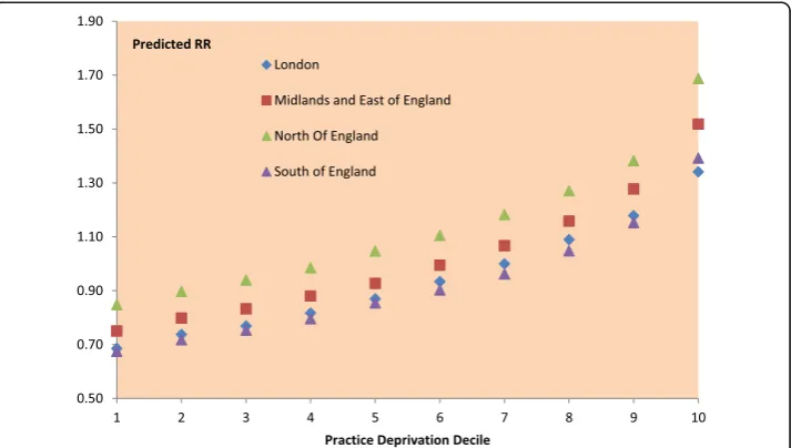
We accordingly disaggregate the 7518 GP practices by their region of location, and according to the England-wide deprivation decile of the practice (that is into 40 subcells). Even in the more affluent South, there are some practices in the highest decile (most deprived practices). Table 7 shows posterior summaries, from the median regression (q = 0.5), regarding average predicted relative risks (RR) for GP practices by subcell. These average RR take into account practice level covariate profiles, and may be affected by satisfaction rates as well as by practice deprivation. It can be seen that, for comparable deprivation levels, GP practice relative risks of ambulatory sensitive emergencies are highest in the North. A risk gradient across ascending deprivation applies across all regions, but steepens in the South at the highest deprivation levels. Figure 1 represents these trends graphically.

A second approach to assessing health care implications is to stipulate particular covariate combinations, and ascertain how these translate into varying relative risks according to region and quantile. To illustrate this, we set transformed practice deprivation to 0.5815 (corresponding to a high IMD score of 40 in the original scale), and the general satisfaction and opening hours satisfaction indicators at their mean values across England. In particular, we focus on the probability, by region, that the

Table 4Fit and model checks

Quantile Model 1 Model 2

0.05 0.5 0.95 0.05 0.5 0.95

Fit

Log predictive density (lpd) ₋27,742 ₋26,643 ₋27,391 ₋27,733 ₋26,644 ₋27,379

Complexity (pwaic) 3387 3764 3723 3385 3771 3725

WAIC 62,258 60,815 62,229 62,235 60,830 62,209

Model Checks

Predictive Coverage (% of observations with 95% CRI of yrepincluding observation)

0.966 1.000 0.975 0.968 1.000 0.976

Posterior Predictive p tests

Log likelihood ratio 0.17 0.45 0.24 0.17 0.43 0.25

Maximum observation 0.47 0.44 0.47 0.46 0.43 0.50

(14)

lower 0.05 quantile for relative risk exceeds 1. Table 8 shows that relative risks for all three quantiles significantly exceed 1 for the North and Midlands regions, but for the 0.05 quantile, the probability that relative risk exceeds 1 in London is inconclusive (at 0.66), and in the South is close to zero.

Slope indices of inequality are measures of health care effectiveness at aggregate level across a set of GP practices. One may also be interested in identifying individual GP practices with elevated ambulatory sensitive admission levels, even after taking account of deprivation and other influences. Thus we can identify those practices with high outlier indicators, Wqi, and in particular those with high ACS admission totals yi, after Table 5Estimated regression coefficients

Posterior summary by quantile and model

Model 1 Model 2

Quantile Mean 2.5% 97.5% Mean 2.5% 97.5%

Intercept 0.05 −0.238 −0.280 −0.195 −0.281 −0.324 −0.230

0.50 −0.086 −0.139 −0.035 −0.113 −0.174 −0.053

0.95 0.074 0.029 0.128 0.076 0.019 0.131

Deprivation 0.05 1.062 1.039 1.088 1.203 1.132 1.285

0.50 1.085 1.053 1.116 1.162 1.082 1.248

0.95 1.110 1.079 1.143 1.103 1.022 1.181

Satisfied Opening Hours 0.05 −0.039 −0.104 0.037 −0.069 −0.156 0.014

0.50 0.022 −0.056 0.103 0.021 −0.062 0.104

0.95 0.145 0.076 0.212 0.143 0.069 0.217

Positive Overall Experience 0.05 −0.450 −0.519 −0.382 −0.429 −0.501 −0.356

0.50 −0.435 −0.509 −0.359 −0.433 −0.511 −0.356

0.95 −0.455 −0.535 −0.388 −0.454 −0.534 −0.386

Differential Intercept Quantile Mean 2.5% 97.5% Mean 2.5% 97.5%

Midlands and East of England 0.05 0.089 0.075 0.105 0.131 0.096 0.172

0.50 0.087 0.071 0.103 0.108 0.073 0.146

0.95 0.092 0.076 0.106 0.078 0.042 0.113

North Of England 0.05 0.199 0.181 0.216 0.263 0.229 0.298

0.50 0.198 0.182 0.213 0.244 0.208 0.282

0.95 0.203 0.188 0.218 0.223 0.186 0.256

South of England 0.05 −0.004 −0.021 0.012 0.041 0.002 0.078

0.50 −0.009 −0.026 0.007 0.007 −0.029 0.044

0.95 −0.006 −0.023 0.009 −0.023 −0.062 0.009

Differential Deprivation Slope Quantile Mean 2.5% 97.5% Mean 2.5% 97.5%

Midlands and East of England 0.05 −0.125 −0.223 −0.041

0.50 −0.062 −0.162 0.036

0.95 0.048 −0.061 0.147

North Of England 0.05 −0.176 −0.264 −0.095

0.50 −0.128 −0.224 −0.037

0.95 −0.049 −0.137 0.055

South of England 0.05 −0.131 −0.236 −0.021

0.50 −0.031 −0.140 0.076

(15)

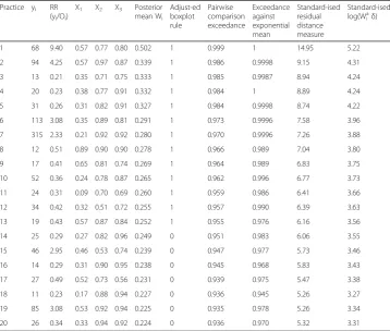
taking account of the covariates and expected events. Table 9 shows response and covariate details for the GP practices with the 20 highest posterior mean W0.5 , i from

the model 2 median regression. Also shown are values for the outlier indicators included in the simulation analysis (section 5). Thus practices 1, 2 and 19 in Table 9 have high yi(and high maximum likelihood relative risks ratios yi/Oi) even after taking

account of covariate values, including high deprivation. Practices 6 and 7 have high yi Table 6Estimated deprivation slopes by region, model 2

Posterior summary by quantile

Quantile Mean 2.5% 97.5%

London 0.05 1.203 1.132 1.285

0.50 1.162 1.082 1.248

0.95 1.103 1.022 1.181

Midlands and East of England 0.05 1.079 1.034 1.127

0.50 1.100 1.051 1.152

0.95 1.152 1.098 1.199

North Of England 0.05 1.028 0.990 1.063

0.50 1.034 0.985 1.081

0.95 1.054 1.007 1.113

South of England 0.05 1.072 0.999 1.135

0.50 1.131 1.055 1.205

0.95 1.185 1.101 1.269

Table 7Estimated relative risks (median quantile regression) for ambulatory sensitive emergency admission by region and deprivation decile of gp practice

Region Decile Number of GP practices

Mean 2.5% 97.5% Region Decile Number of GP practices

Mean 2.5% 97.5%

London 1 70 0.69 0.67 0.70 North 1 109 0.85 0.83 0.86

2 90 0.74 0.72 0.75 2 155 0.90 0.88 0.91

3 105 0.77 0.75 0.78 3 163 0.94 0.93 0.95

4 117 0.82 0.80 0.83 4 168 0.99 0.97 1.00

5 132 0.87 0.86 0.88 5 181 1.05 1.04 1.06

6 184 0.93 0.92 0.94 6 201 1.11 1.10 1.12

7 180 1.00 0.99 1.01 7 261 1.18 1.17 1.19

8 222 1.09 1.07 1.11 8 292 1.27 1.26 1.28

9 205 1.18 1.16 1.20 9 294 1.38 1.37 1.40

10 51 1.34 1.31 1.38 10 445 1.69 1.66 1.72

Midlands-East 1 232 0.75 0.74 0.76 South 1 340 0.67 0.66 0.69

2 239 0.80 0.79 0.81 2 268 0.72 0.71 0.73

3 229 0.83 0.82 0.84 3 255 0.75 0.75 0.76

4 273 0.88 0.87 0.89 4 194 0.80 0.79 0.80

5 235 0.93 0.92 0.94 5 203 0.85 0.85 0.86

6 215 0.99 0.99 1.00 6 152 0.90 0.89 0.92

7 192 1.07 1.06 1.08 7 119 0.96 0.95 0.98

8 167 1.16 1.15 1.17 8 71 1.05 1.03 1.07

9 207 1.28 1.26 1.30 9 46 1.15 1.12 1.18

(16)

despite average or below average deprivation. Practices 8, 9, 13, 17 and 19 have low yi

despite high deprivation. Most other extreme outliers in Table 9 have unduly low yi.

There are 13 outlier practices (the first 13 practices in Table 9) according to the ad-justed boxplot method of Hubert and Vandervieren (2008), which is applied to posterior mean W0.5 , i. Other methods provide less restrictive definitions. A cut off of 3 for

standar-dised Uqi= log(Wqiδq) (cf. Table 3) leads to 42 observations being classed as outliers, and a

cut off of 3 for standardised residual distance measures leads to 114 outliers.

As a sensitivity analysis, alternative priors were assumed on the exponential scale parameters δq. Instead of the gamma Ga (1,0.001) prior, a uniform prior on δq is

considered, δq~ U(0, 10000), and also parameterisation in terms of exponential

means ϕq= 1/δq. Thus Wqi∼exp(1/ϕq), log(ϕq) =ω0q, with ω0q assigned a diffuse

normal N (0,1000) prior. Table 10 shows that the posterior δq are very similar

under the different priors, and other inferences are not affected.

Fig. 1Hierarchical median regression. Predicted ACS relative risks by region and deprivation decile

Table 8Predicted relative risks (RR) by region, specified values predictor combination

Posterior summary by quantile and region

Mean 2.5% 97.5% Prob(RR > 1|Y)

q = 0.05 London 1.006 1.006 1.026 0.663

Midlands/East 1.064 1.063 1.076 1

North 1.170 1.170 1.184 1

South 0.964 0.963 0.991 0.002

q = 0.50 London 1.234 1.234 1.262 1

Midlands/East 1.327 1.328 1.349 1

North 1.463 1.463 1.483 1

South 1.223 1.223 1.261 1

q = 0.95 London 1.557 1.557 1.588 1

Midlands/East 1.732 1.733 1.757 1

North 1.898 1.898 1.922 1

(17)

8. Conclusions

In this paper, a model for quantile regression within a hierarchical Poisson lognormal framework is proposed for overdispersed count responses. This technique has the advantage that a profile of incidence rates or relative risks across quantiles can be obtained, taking account of quantile specific covariate effects, and including estimates of uncertainty (e.g. the uncertainty attaching to lower and upper relative risk quantiles). Among methodological extensions that may be included are varying Wqi according to

case specific covariates, and covariate selection.

A simulation in R using known regression coefficients shows the technique accurately estimates the true regression coefficients when the data are contaminated by outliers,

Table 9Leading GP practice outliers, median regression, ambulatory sensitive emergency admissionsa

Practice yi RR (yi/Oi)

X1 X2 X3 Posterior mean Wi

Adjust-ed boxplot rule

Pairwise comparison exceedance

Exceedance against exponential mean

Standard-ised residual distance measure

Standard-ised log(Wiaδ)

1 68 9.40 0.57 0.77 0.80 0.502 1 0.999 1 14.95 5.22

2 94 4.25 0.57 0.97 0.87 0.339 1 0.986 0.9998 9.15 4.31

3 13 0.21 0.35 0.71 0.75 0.333 1 0.985 0.9987 8.94 4.24

4 20 0.23 0.38 0.77 0.91 0.332 1 0.984 1 8.89 4.24

5 31 0.26 0.31 0.82 0.91 0.327 1 0.984 0.9998 8.74 4.22

6 113 3.08 0.35 0.89 0.81 0.291 1 0.973 0.9996 7.58 3.96

7 315 2.33 0.21 0.92 0.92 0.280 1 0.970 0.9996 7.26 3.88

8 12 0.51 0.89 0.90 0.90 0.278 1 0.966 0.989 7.04 3.80

9 17 0.41 0.65 0.81 0.74 0.269 1 0.964 0.989 6.83 3.75

10 52 0.36 0.24 0.78 0.87 0.265 1 0.962 0.996 6.77 3.73

11 24 0.31 0.09 0.70 0.69 0.260 1 0.959 0.986 6.41 3.66

12 34 0.42 0.32 0.51 0.72 0.255 1 0.957 0.990 6.39 3.63

13 19 0.43 0.57 0.87 0.84 0.252 1 0.955 0.976 6.16 3.56

14 25 0.29 0.27 0.82 0.96 0.249 0 0.951 0.983 6.06 3.55

15 46 2.95 0.46 0.53 0.74 0.239 0 0.947 0.977 5.73 3.46

16 14 0.29 0.31 0.90 0.95 0.238 0 0.945 0.968 5.83 3.43

17 27 0.49 0.52 0.73 0.56 0.231 0 0.939 0.975 5.47 3.38

18 11 0.23 0.17 0.88 0.94 0.227 0 0.936 0.945 5.26 3.27

19 85 3.08 0.53 0.92 0.94 0.225 0 0.935 0.978 5.26 3.34

20 26 0.34 0.33 0.94 0.92 0.224 0 0.936 0.970 5.32 3.31

a_{Average values for X1-X3 are 0.33, 0.79 and 0.85}

Table 10Estimatedδqunder different priors (Model 2)

Quantile (q) Mean Std devn 2.5% 97.5%

Gamma prior 0.05 85.57 1.49 82.78 88.51

0.50 13.13 0.18 12.76 13.49

0.95 71.83 1.13 69.64 74.13

Uniform prior 0.05 85.37 1.38 82.70 88.12

0.50 13.12 0.18 12.77 13.49

0.95 71.85 1.09 69.74 74.06

0.50 13.11 0.19 12.74 13.48

(18)

with performance comparable to that of Aeberhard et al. (2014). The technique also accurately identifies the sample observations subject to contamination.

A real application focuses on estimating central, low and high quantile regressions for levels of ambulatory sensitive emergency admissions across English GP practices. Practice deprivation is the strongest predictor of such emergency admissions, and the deprivation effect varies by quantile under the second model considered for these data. In particular, using stipulated values for covariates, it was shown that relative risks for all quantiles significantly exceed 1 for the Midlands-East and North, but for the 0.05 quantile, the probabilities that relative risk exceeds 1 in London and the South are zero or inconclusive. Outlier GP practices (in the response space) were also identified.

The methodology used in the paper may have utility in other health applications where institutional or regional variations in health outcomes are of policy concern.

Additional file

Additional file 1:Appendix 1. Sample Size for Simulations. Appendix 2. R Code for Simulations. (DOCX 23 kb)

Acknowledgements

We appreciate for the reviewers’insightful comments, which helped to improve the paper.

Funding

There are no funding sources.

Authors_’contributions

PC conceived of the method, performed the statistical analysis, and drafted the manuscript.

Competing interests

The author declares that he has no competing interests.

Publisher’s Note

Springer Nature remains neutral with regard to jurisdictional claims in published maps and institutional affiliations.

Received: 4 May 2017 Accepted: 27 July 2017

References

Aeberhard, W, Cantoni, E, Heritier, S: Robust inference in the negative binomial regression model with an application to falls data. Biometrics.70(4), 920–931 (2014)

Agostinelli, C, Greco L: A weighted strategy to handle likelihood uncertainty in Bayesian inference. Comput. Stat.28(1), 319-339 (2013)

Andersen, R: Modern methods for robust regression. Sage Publishing (2008)

Benites, L, Lachos, V, Vilca, F: Case-deletion diagnostics for Quantile regression using the asymmetric Laplace distribution. arXiv preprint arXiv.1509, 05099 (2015)

Benoit, D, Van den Poel, D: Binary quantile regression: a Bayesian approach based on the asymmetric Laplace distribution. J. Appl. Econometrics.27(7), 1174_–1188 (2012)

Berkhof, J, Van Mechelen, I, Hoijtink, H: Posterior predictive checks: principles and discussion. Comput. Stat.15(3), 337_–354 (2000)

Bondell, H, Reich, B, Wang, H: Noncrossing quantile regression curve estimation. Biometrika.97(4), 825–838 (2010) Brooks, S, Gelman, A: General methods for monitoring convergence of iterative simulations. J. Comput. Graphical Stat.

7(4), 434–455 (1998)

Caminal, J, Starfield, B, Sánchez, E, Casanova, C, Morales, M: The role of primary care in preventing ambulatory care sensitive conditions. Eur. J. Public Health.14(3), 246–251 (2004)

Carling, K: Resistant outlier rules and the non-Gaussian case. Comput. Stat. Data Anal.33(3), 249_–258 (2000) Chambers, R, Dreassi, E, Salvati, N: Disease mapping via negative binomial regression M-quantiles. Stat. Med.33(27),

4805_–4824 (2014)

Connolly, S, Dornelas, M, Bellwood, D, Hughes, T: Testing species abundance models: a new bootstrap approach applied to indo-Pacific coral reefs. Ecology.90(11), 3138_–3149 (2009)

Connolly, S, Thibaut, L: A comparative analysis of alternative approaches to fitting species abundance models. J. Plant Ecol.5, 32_–45 (2012)

(19)

Dolton, P, Pathania, V: Can increased primary care access reduce demand for emergency care? Evidence from England’s 7-day GP opening. J. Health Econ.49, 193–208 (2016)

Gelfand, A: Model determination using sampling-based methods, In: Gilks, PW, Richardson, S, Spiegelhalter, D (eds.) Markov Chain Monte Carlo. Chapman & Hall/CRC, Boca Raton (1996)

Greco, L, Racugno, W, Ventura, L: Robust likelihood functions in Bayesian analysis. J. Stat. Plan. Inf.138, 1258–1270 (2008)

Hilbe, J: Negative Binomial Regression, 2nd edition. Cambridge University Press, Cambridge (2011) Huber, P: Robust regression: asymptotics, conjectures and Monte Carlo. Ann. Stat.1(5), 799–821 (1973) Hubert, M, Vandervieren, E: An adjusted boxplot for skewed distributions. Comput. Stat. Data Anal.52(12),

5186–5201 (2008)

Koenker, R, Hallock, K: Quantile regression. J. Econ. Perspect.15, 143–156 (2001)

Lunn, D, Thomas, A, Best, N, Spiegelhalter, D: WinBUGS–a Bayesian modelling framework: concepts, structure, and extensibility. Stat. Comput.10, 325–337 (2000)

Machado, J, Santos Silva, J: Quantiles for counts. J. Am. Stat. Assoc.100(472), 1226–1237 (2005)

Miranda-Moreno, L, Fu, L, Saccomano, F, Labbe, A: Alternative risk model for ranking locations for safety improvement. Transportation Res. Record.1908, 1–8 (2005)

Moreno, E, Pericchi, L: Bayesian robustness for hierarchicalɛ-contamination models. J. Stat. Plan. Inf.37, 159–168 (1993) Regidor, E: Measures of health inequalities: part 2. J. Epidemiol. Community Health.58(11), 900–903 (2004)

Reich, B, Fuentes, M, Dunson, D: Bayesian spatial quantile regression. J. Am. Stat. Assoc.106(493), 6–20 (2011) Richardson, S, Thomson, A, Best, N, Elliott, P: Interpreting posterior relative risk estimates in disease-mapping studies.

Environ. Health Perspect.112, 1016–1025 (2004)

Ruopp, M, Perkins, N, Whitcomb, B, Schisterman, E: Youden index and optimal cut-point estimated from observations affected by a lower limit of detection. Biom. J.50(3), 419–430 (2008)

Santos, B, Bolfarine, H: On Bayesian quantile regression and outliers. arXiv preprint arXiv.1601, 07344 (2016) Sheringham, J, Asaria, M, Barratt, H, Raine, R, Cookson, R: Are some areas more equal than others? Socioeconomic

inequality in potentially avoidable emergency hospital admissions within English local authority areas. J. Health Serv. Res. Policy.22(2), 83–90 (2016)

Sohn, S: A comparative study of four estimators for analyzing the random event rate of the Poisson process. J. Stat. Comput. Simul.49(1–2), 1–10 (1994)

Takeuchi, I, Le, Q, Sears, T, Smola, A: Nonparametric quantile estimation. J. Mach. Learn. Res.7, 1231–1264 (2006) Tian, Y, Dixon, A, Gao, H: Emergency Hospital Admissions for Ambulatory Care-Sensitive Conditions: Identifying the

Potential for Reductions. King’s Fund, London (2012). https://www.kingsfund.org.uk/ Tsionas, E: Bayesian quantile inference. J. Stat. Comput. Simul.73, 659–674 (2003)

Verardi, V, Vermandele, C: Outlier identification for skewed and/or heavy-tailed unimodal multivariate distributions. J. de la Société Française de Statistique.157(2), 90–114 (2016)

Wang, C, Blei, D: A general method for robust Bayesian modeling. Bayesian Anal (forthcoming). (2017)

Watanabe, S: Asymptotic equivalence of Bayes cross validation and widely applicable information criterion in singular learning theory. J. Mach. Learn. Res.11, 3571–3594 (2010)

Wilcox, R: Understanding and Applying Basic Statistical Methods Using R. John Wiley, Hoboken (2016) Wu, Y, Liu, Y: Stepwise multiple quantile regression estimation using non-crossing constraints. Stat. Interface.

2, 299–310 (2009)