Occlusion-Aware View Interpolation

Volume 2008, Article ID 803231,15pages doi:10.1155/2008/803231

Research Article

Occlusion-Aware View Interpolation

Serdar Ince1, 2_{and Janusz Konrad (EURASIP Member)}1

1_{Department of Electrical and Computer Engineering, Boston University, 8 Saint Mary’s Street, Boston, MA 02215, USA} 2_{IntelliVid Corporation, Cambridge, MA 02138, USA}

Correspondence should be addressed to Janusz Konrad,[email protected]

Received 3 March 2008; Accepted 1 October 2008

Recommended by Peter Eisert

View interpolation is an essential step in content preparation for multiview 3D displays, free-viewpoint video, and multiview image/video compression. It is performed by establishing a correspondence among views, followed by interpolation using the corresponding intensities. However, occlusions pose a significant challenge, especially if few input images are available. In this paper, we identify challenges related to disparity estimation and view interpolation in presence of occlusions. We then propose an occlusion-aware intermediate view interpolation algorithm that uses four input images to handle the disappearing areas. The algorithm consists of three steps. First, all pixels in view to be computed are classified in terms of their visibility in the input images. Then, disparity for each pixel is estimated from different image pairs depending on the computed visibility map. Finally, luminance/color of each pixel is adaptively interpolated from an image pair selected by its visibility label. Extensive experimental results show striking improvements in interpolated image quality over occlusion-unaware interpolation from two images and very significant gains over occlusion-aware spline-based reconstruction from four images, both on synthetic and real images. Although improvements are obvious only in the vicinity of object boundaries, this should be useful in high-quality 3D applications, such as digital 3D cinema and ultra-high resolution multiview autostereoscopic displays, where distortions at depth discontinuities are highly objectionable, especially if they vary with viewpoint change.

Copyright © 2008 S. Ince and J. Konrad. This is an open access article distributed under the Creative Commons Attribution License, which permits unrestricted use, distribution, and reproduction in any medium, provided the original work is properly cited.

1. INTRODUCTION

The generation of a novel (virtual) view of a scene captured by real cameras is often referred to asimage-based rendering. The problem is illustrated for the case of two cameras in Figure 1. The goal is to reconstruct image J, that would have been captured by camera CJ had it been used, based on images IL and IR captured by cameras CL and CR, respectively. Generation of such views is an essential step in content preparation for multiview 3D displays [1–3], free-viewpoint video [4,5], and multiview compression [6–8]. A very similar problem exists in frame-rate conversion of video, except that novel images are created from diff erent-time snapshots rather than different views.

In order to render novel view, first a correspondence among known views needs to be established followed by an estimation of new intensity from the known intensities in correspondence. Depending on how the correspondence mapping is defined, two approaches are possible. One approach is based onbackward projectionof intensities (the

to scene structure, for example, areaA inILis occluded in IR (seeFigure 1). Note that a disappearing area becomes an appearing area (also known as uncovered ornewly-exposed area), and vice versa, if the order of views is reversed, that is, “right-to-left” instead of “left-to-right.”

Many approaches to novel view generation have been proposed to date. Although some methods account for occlusions, few handle occlusions accurately. Consequently, occlusion areas are recovered inaccurately. Our motivation in this paper is to improve the novel image quality in occlusion areas. This is somewhat easier in approaches based on forward projection since the correspondence mapping is defined in the coordinate system of known images, and thus known luminance/color can be used to reason about the presence/absence as well as nature of occlusions. We have recently developed successful methods in this category [9,10]. On the other hand, in backward-projection methods the mapping is defined in the coordinate system of a novel image and thus no luminance/color is available to reason about occlusions. We address this difficulty here. We propose a new occlusion-aware backward-projection view interpolation. The method first identifies pixel visibility in the intermediate image, that is, whether a particular pixel is visible in all input images or only in those to the left or to the right of the image to be reconstructed. These labels are incorporated into a variational formulation to adaptively choose different pairs of input images and reliably estimate disparity under anisotropic regularization constraint. The final view generation is accomplished by occlusion-adaptive linear intensity interpolation.

The paper is organized as follows. In Section 2, we review prior work on intermediate view interpolation and reconstruction as well as occlusion detection. In Section 3, we present the new occlusion-aware view interpolation, and inSection 4, we show experimental results. InSection 5, we discuss benefits and deficiencies of forward- and backward-projection approaches, and inSection 6, we summarize the paper and draw conclusions.

2. PRIOR WORK

Image-based rendering is concerned with creating an image at a specific 3D location and specific time. Adelson and Bergen [11] formulated a description for all possible images by means of the so-called plenoptic function that records light rays at every possible 3D location, in every possible direction, at every time instant, and for all wavelengths. In order to generate a new image, one simply needs to sample this 7-dimensional function. However, capturing a full plenoptic function is difficult, if not impossible, and thus various assumptions aiming at the reduction of this high dimensionality have been proposed. For example, if only static scenes are considered in grayscale, the number of dimensions reduces to five.

Although prior work can be classified based on the number of dimensions of a plenoptic function used [12], in the context of work proposed, here we prefer to classify prior methods based on their need for structure information and the number of input images.

(1)Methods that rely on oversampling.Among the most prominent methods that rely on scene oversampling are lightfield rendering [13] and lumigraph [14]. Both methods create a 4D representation of the scene using many input images. The novel views are created by slicing (sampling) this 4D representation. Since the scene is oversampled, the rendering process simply blends the input images, ignoring scene structure. The presence of occlusions is not a problem because, thanks to oversampling, occlusions between nearest cameras are negligible, and all texture in the scene is visible from several cameras.

(2)Methods that use undersampled data sets with known structure.Given the scene structure, it is possible to reduce the required number of images [15–18]. If the depth map or 3D model of a scene is available, it is possible to project pixels of the known images to a new viewpoint and reconstruct a new image. Obviously, it is not guaranteed that all pixels in the new image will be visible in the input images. However, since the scene structure is known, locations of occlusions are known, which is not the case considered in this paper.

(3)Methods that use severely undersampled data sets with unknown structure.These methods have no access to scene structure and use few input images, typically 2–4. The scene structure is computed implicitly (from disparity) either using correspondence matching or projective geometry. These methods can be categorized based on what approach they use to estimate the disparity: methods based on projective geometry or rectification [19–21], methods based on optical flow [5,9,22,23], methods based on block correspondence: variable-size blocks [24], fixed-size blocks [25], sliding blocks [26], methods based on feature correspondence [27], and methods using dynamic programming [28]. Because of limited input data and unknown scene structure, the reconstruction problem is ill-posed and requires some from of the regularization, usually by means of additional constraints. The work presented in this paper is closest to this class of methods.

2.1. Forward- and backward-projection methods

When computing an intermediate view, the central role is played by a transformation between the coordinate systems of known images and the novel image. This transformation depends on camera geometry and scene structure, and is usually unknown. It can be estimated by solving the correspondence problem with two possible definitions of the transformation: from known to novel image coordinates, also calledforward projection, or from novel to known image coordinates, calledbackward projection.

CL CJ CR

(a)

IL J IR

A A B B

(b)

IL J IR

A

B

(c)

Figure1: Illustration of intermediate view reconstruction from two cameras: (a) camera setup (CJis a virtual camera, whileCLandCRare

real cameras), (b) occlusion effect in captured images, and (c) occlusion effect in one row of pixels from the images. AreaAfromILis being

occluded inIRby the object, while areaBis being uncovered (areaBwould undergo occlusion had the direction of arrows been reversed).

IL J IR

α 1−α

(a)

IL J IR

α 1−α

(b)

IL J IR

α 1−α

(c)

Figure2: Disparity vectors defined (pivoted) in: (a) left (known), (b) right (known), and (c) intermediate (unknown) images.

2.1.1. Forward projection

Disparity vectors (transformation) are defined in the coor-dinate system of known images. LetdLbe a disparity field defined on lattice Λ of IL (see Figure 2(a)), and let dR be defined on lattice Λ of IR (see Figure 2(b)). Under the constant-brightness assumption [29], the following holds

IL(x)=IRx+dL(x), IR(x)=ILx+dR(x), ∀x∈Λ. (1)

Assuming that brightness constancy holds along the whole disparity vector, also the following is true:

Jx+αdL(x)

=IL(x),

Jx+ (1−α)dR(x)=IR(x), ∀x∈Λ. (2)

Clearly, the reconstruction of intermediate-view intensities J(x +αdL(x)) and J(x + (1 −α)dR(x)) can be as simple as substitution withIL(x) andIR(x), respectively. However, in general, x + αdL(x)∈/ Λ and x + (1 − α)dR(x)∈/Λ, that is, the projected points are off lattice Λ. In fact, due to the space-variant nature of disparities, the above locations are usually irregularly spaced, whereas the goal is to reconstructJ(x) regularly spaced (x ∈ Λ). One option is to force the locations x+αdL(x) andx+ (1−α)dR(x) to belong to Λ. For orthonormal lattices typically used,

this means forcing αdL(x) and (1− α)dR(x) to be full-pixel vectors, that is, rounding coordinates to the nearest integer [21,25]. Advanced approaches, such as those using splines to perform irregular-to-regular conversion, have also been proposed [9]. While simple rounding suffers from objectionable reconstruction errors, advanced spline-based methods produce high-quality reconstructions but require significant computational effort.

2.1.2. Backward projection

Disparity vectors are defined in the coordinate system of the intermediate image J, and bidirectionally point toward the known images [24, 30, 31]. As shown in Figure 2(c), dJ is defined on Λ in J thus forcing disparity vectors to pass through pixel positions of the intermediate view (i.e., vectors arepivotedin the intermediate view). The constant-brightness assumption now becomes

ILx−αdJ(x)

=IRx+ (1−α)dJ(x)

, ∀x∈Λ. (3)

Compared to (1), each pixel inJis guaranteed to be assigned a disparity vector and, therefore, two intensities (fromILand IR) associated with it. Although usuallyx−αdJ(x)∈/Λand x+ (1−α)dJ(x)∈/ Λ, intensities at these points can be easily calculated fromILandIRusing spatial interpolation.

estimation for eachα, it also simplifies the final computation ofJ. The reason is that view rendering becomes a byproduct of disparity estimation; once dJ that satisfies (3) is found, either left or right luminance/color can be used for the intermediate-view texture. An even better reconstruction is accomplished when weighted averaging (linear interpola-tion) of both intensities is applied [24,32]

J(x)=(1−α)ILx−αdJ(x)

+αIRx+ (1−α)dJ(x)

, ∀x∈Λ. (4)

Clearly, all intermediate-view pixels are assigned an intensity, and postprocessing is not needed.

2.2. Occlusion-aware image-based rendering

In the case of oversampled data sets, if occlusions can be reliably identified, then selection of visible features is not difficult (many views are available). In fact, explicit detection of occlusions is not even necessary; robust photo-consistent measures embedded into the rendering algorithm are sufficient [33].

In the case of undersampled data sets, the situation is different, especially when scene structure (depth) is unknown. In fact, occlusions have dual impact in this case. First, correspondence (disparity) is not defined in occlusion areas, and thus some a priori assumptions must be made about correspondences (e.g., smoothness). Secondly, during the estimation of disparities unreliable estimates in occlusion areas impact the outcome at neighboring positions, thus spreading the occlusion-related errors. Know-ing where occlusions take place can help correctKnow-ing both problems.

In forward-projection methods, pixels from IL (see Figure 2(a)) orIR (seeFigure 2(b)) that are occluded in the other image can be assigned a disparity based on depth constancy assumption [34], that does not work well at object boundaries, or by means of edge-preserving disparity inpainting [9], that has been shown to be more accurate. The latter approach is possible since disparities are defined in the coordinate system of known images (ILorIR), and thus their underlying gradients can be used to guide anisotropic disparity diffusion that improves the quality of estimated disparities (discontinuities) [35,36].

In backward-projection methods, disparity is defined in the coordinate system of the unknown image J, and no underlying gradients are available to permit anisotropic diffusion. Therefore, the estimated disparities are usually excessively smooth. Although robust error metrics can be used in regularization [37], this is often insufficient. Moreover, it is unclear how to identify occlusions using a single disparity field. These are the main issues we address in this paper.

As for occlusion detection, it usually exploits one of several constraints. An ordering constraint preserves pixel order on corresponding rows of left and right images [38] but cannot handle thin foreground objects or narrow holes. A uniqueness constraint assures one-to-one mapping of pixels on corresponding rows [39]. In one implementation,

it relies on the geometry of disparity fields; a significant difference between forward (e.g., left-to-right) and back-ward (e.g., right-to-left) disparity vectors is indicative of occlusions [40]. This constraint can also be thought of as a geometric constraint as it relies on the analysis of disparity field geometry. Some other geometric constraints assume that disparity varies smoothly everywhere except object boundaries (continuity constraint) [39], or that occlusion areas exhibit excessive disparity gradient [41]. Yet another geometric constraint seeks uncovered pixels in IR by inspecting an irregular grid of forward disparity-compensated pixels of image IL. This constraint has been shown to be very effective and noise resilient in occlusion detection [42]. A related, although weaker, visibility con-straint [43] also assures consistency of uncovered pixels in one image with disparity of the other image, but it permits many-to-one matches in visible areas. Finally, aphotometric constraint (or constant-brightness constraint [29]) ensures intensity match in visible areas. It is the simplest indicator of occlusions but prone to errors in presence of image noise and illumination changes. Methods based on multiple views compare intensity consistency along a path formed by displacement vectors in 3 or more frames [44–46]. Graph cuts have also been used in multiview occlusion detection [47].

3. OCCLUSION-AWARE BACKWARD-PROJECTION VIEW INTERPOLATION

In backward-projection methods, disparities estimated around occlusion areas are erroneous since no underly-ing image gradients are available. Lack of image gradient prevents the use of edge-preserving (anisotropic) diffusion. Below, we argue that by using a coarse estimate of the intermediate image the fidelity of disparity field can be significantly improved around occlusion areas. With this capacity to compute more accurate disparities, we then propose a new approach to occlusion-aware backward-projection view interpolation.

3.1. Edge-preserving disparity regularization using a coarse intermediate image

is the true intermediate image. Disparity, estimated using simple isotropic regularization:

arg min

d(x)

x∈ΩJ

IL(x−αd(x)−IRx+ (1−α)d(x)2

+λ∇u2_+∇v2_dx,

(5)

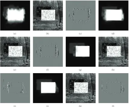
whereΩJ is the domain ofJ, d(x) = [u(x) v(x) ]T, and ∇is the gradient operator, is shown inFigure 3(d). Clearly, it is excessively smooth.Figure 3(e) shows an intermediate image computed by using this disparity in (4). Although there are significant texture errors (as clear fromFigure 3(f)), edge maps, obtained using the Canny edge detector, are very similar for the true and reconstructed intermediate images (see Figures3(g) and3(h)).

Therefore, we propose to use a coarse intermediate image Jc, computed using isotropically-diffused disparities (5), to guide edge-preserving regularization as follows:

arg min

d(x)

x∈ΩJ

ILx−αd(x)−IRx+ (1−α)d(x)2

+λFx

u,Jc+Fx

v,Jcdx.

(6)

Above, Fx(·) assures anisotropic regularization [50] and is

defined as follows:

Fx

u,Jc= ∇T_u(x) ⎡

⎣gJcx(x) 0 0 gJcy(x)

⎤ ⎦_∇u(x),

(7)

whereg(·) is a monotonically decreasing function, andJx c,J

y c are horizontal and vertical derivatives ofJcatx. If|Jx

c(x)| = |Jcy(x)|, then isotropic smoothing takes place ((6) simplifies to (5), except for different λ). However if, for example, |Jx

x(x)| |J y

c(x)| then stronger smoothing takes place vertically, and the vertical edge is preserved.

The disparity field shown inFigure 3(i) was computed using formulation (6). It is clear that the object shape is very well preserved. The intermediate view obtained using this disparity field in backward projection (4) and its interpolation error are shown in Figures3(j) and3(k), respectively. As is clear from error images, distortions along the horizontal boundaries of the square are suppressed compared to Figure 3(f) because the excessive smoothness of disparity field is eliminated. Although these are nonoc-cluding boundaries, they were assigned incorrect disparities due to isotropic regularization (5). Edge-preserving regular-ization (6) corrected the problem, and these areas are now assigned accurate disparities. Consequently, the intermediate image is properly reconstructed there. Significant errors, however, persist in occlusion areas (vertical boundaries, see Figure 3(k)). This is due to occlusion unawareness of the algorithm; a point is visible only in one of the images, but reconstruction based on backward projection (4) averages intensities from both images. Therefore, next we propose to use additional images to solve for occlusion areas.

3.2. Backward-projection view interpolation using multiple images

In order to improve reconstruction in occlusion areas, we first need to estimate their locations, and then figure out what intensities belong there. Without loss of generality, let us consider four input images as shown inFigure 4. Although this is a simple scenario, it does convey the main idea we intend to pursue. While the top row shows images containing a black square against background containing areasAandB, the bottom row shows their horizontal cross-sections (rows of pixels). The goal is to reconstruct the intermediate image Jusing input imagesI1, I2, I3, andI4. Note that areasAand

Bare being occluded/exposed between the four images. In occlusion-unaware interpolation (4),I2andI3would

be the input images, and a disparity field defined onJwould be estimated. For most points inJ, it is possible to estimate accurate disparities because the corresponding points are visible in bothI2andI3. However, areasAandBare occluded

in eitherI2orI3, and it is not possible to estimate disparities

there. Note that areasAandBare visible in additional images to the left of I2 and to the right of I3. Thus, it should be

possible to estimate disparities in areaAusingI1andI2, and

disparities in areaBusingI3andI4. Therefore, a formulation

is needed to estimate disparities ofJ by choosing between three image pairs: (I1,I2), (I3,I4), or (I2,I3).

In order to implement switching between image pairs, one first needs to identify areas A and B. We propose to use a method that we had developed earlier [42]. Given a disparity field between two images, this method identifies areas that will be exposed between images, and such areas are equivalent to occluded areas when target and reference images are interchanged. The method is based on the fact that pixels in the target image, that did not exist in the reference image (i.e., newly-exposed pixels), have no relationship to the reference image and, as such, cannot be pointed to by disparity vectors. Thus, when pixels of reference image are forward disparity compensated onto target image, these areas are empty and can be easily detected. Since we need to identify areas that disappear to the left and to the right ofJ, we must estimate two disparity fields: d12defined inI1and pointing toI2, andd43defined inI4and

pointing toI3. We use formulation (6) withI1 (I4) used for

edge-preserving regularization when computingd12(d43).

Our occlusion detection method [42] yields the areaBby using (1+α)d12. The coefficient (1+α) is needed to normalize

the disparity field so that it is correctly mapped ontoJ (see Figure 4). The estimated areaBis exposed between I1 and

J, and, therefore, visible inI3 andI4. Similarly, using (2−

α)d43yields areaA, which is visible inI1andI2. LetL(x) be

a visibility label at locationxinJ that we wish to estimate. Clearly, by usingd12andd34, we can label all points inJas

visible inI1andI2only (L(x)= −1), visible inI3andI4only

(L(x) = 1), or visible inI2 andI3 (L(x) = 0). (The actual

label values have no importance; other values, such as 1, 2, and 3, could have been chosen.)

(a) (b) (c) (d)

(e) (f) (g) (h)

(i) (j) (k)

Figure3: Results of backward-projection view interpolation for synthetic sequence no.1 with horizontal disparity: (a)IL, (b) ground-truth J, (c)IR, (d) disparity estimated using isotropic diffusion (5), (e)Jinterpolated using (4) with disparity from (d), (f) interpolation error for Jfrom (e), (g) edge map of ground-truth imageJ, (h) edge map of interpolated imageJ, (i) disparity estimated using anisotropic diffusion

(6) withJcfrom (e), (j)Jinterpolated using (4) with disparity from (i), (k) interpolation error forJfrom (j). SeeTable 1for PSNR values of

the interpolation error.

regularization. We first define matching errors for image pairs (I1,I2), (I2,I3), and (I3,I4) as follows:

θ12(x)=I1

x−(1 +α)d(x)−I2

x−αd(x), θ23(x)=I2

x−αd(x)−I3

x+ (1−α)d(x), θ34(x)=I3

x+ (1−α)d(x)−I4

x+ (2−α)d(x). (8)

The coefficients (1 −α), (1 +α), (2−α) adjust disparity vectors depending on the distance toJ. For locationsx∈ΩJ outside ofAandB, all three errors yield small magnitudes. However, in occlusion areas only one of them will have a small magnitude. For example, for x in area A, θ12(x)

will have a small magnitude, whereas for x in area B the magnitude ofθ34(x) will be small.

In order to estimate disparities either bidirectionally (visible pixels) or unidirectionally (occlusion areas), we propose the following variational formulation that controls

intensity matching using labels L under edge-preserving regularization:

min

d E, E=

x∈ΩJ

eP(x) +λeS(x)dx (9)

with

eP(x)=P12(x) +P23(x) +P34(x),

eS(x)=Fx

u,Jc+Fx

v,Jc, (10)

P12(x)=δ

L(x) + 1θ12(x)

2

,

P23(x)=δ

L(x)θ23(x)

2

,

P34(x)=δ

L(x)−1θ34(x)

2

,

(11)

whereFx is defined in (7),Jcis a coarse intermediate image

I1 I2 J I3 I4

A A B A B A B B

1 α 1−α 1

A

Visible

B Visible I1 I2 J I3 I4

Figure 4: Illustration of how to use four images in backward-projection intermediate view interpolation. AreasAandBcan be estimated inJ using (I1,I2) and (I3,I4), respectively, while points

outside ofAorBcan be estimated using (I2,I3).

if L(x) = −1, then P12(x) is used. Since Kronecker delta

δ(x) is not differentiable, we use an approximation, such as δ(x) = limk→ ∞e−kx2 (k=1010 _{gives good approximation).}

The derivation of Euler-Lagrange equations for the above variational formulation is included in the appendix.

Once the disparity field has been estimated, it is possible to reconstruct J by using any intensity value along the disparity vector, but averaging leads to better results (noise suppression). We propose to reconstruct the intermediate viewJas follows:

J(x)=δL(x) + 1ξ12+δ

L(x)ξ23

+δL(x)−1ξ34 ∀x∈ΩJ,

(12)

where ξ· are intensity averages along disparity vector d(x) defined as follows:

ξ12=

1 2

I1

x−(1 +α)d(x)+I2

x−αd(x),

ξ23=1

2

I2

x−αd(x)−I3

x+ (1−α)d(x),

ξ34=

1 2

I3

x+ (1−α)d(x)−I4

x+ (2−α)d(x). (13)

Note that at everyx, only one of the values in (13) contributes toJ(x) (12) because of theδ(·) terms.

4. EXPERIMENTAL RESULTS

We solve partial differential equations derived in the appendix using explicit discretization with a small time step dt=1.5×10−5and 11×103iterations. We employ a 4-level hierarchical implementation in order to avoid local minima, and bicubic interpolation to estimate subpixel intensities. In all experimental results shown in the paper, we use λ = 2000. Compared to the disparity estimation step (9), the final view interpolation (12) is very simple and requires little computation.

In order to gauge gains due to the use of 4 images, we have compared the proposed algorithm with view interpolation based on 2-image backward projection with isotropic as well as edge-preserving regularization of disparities (see Section 3.1). We have also compared our algorithm with equivalent forward-projection reconstruction using the same 4 images [9]. The method uses occlusion-aware edge-preserving estimation of 3 disparity fields (from (I1,I2),

(I2,I3), and (I3,I4)), followed by occlusion detection, and

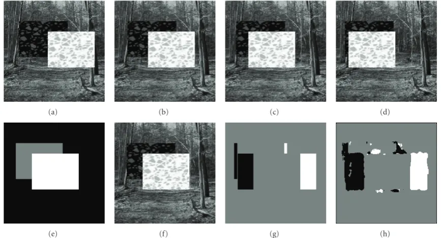
spline-based image reconstruction. A listing of tested algo-rithms along with corresponding objective metrics (PSNR of interpolation error, i.e., difference between the ground-truth and computed intermediate images) can be found inTable 1. In the first test, we generated two additional images for the synthetic test sequence shown inFigure 3. The four input images are shown in Figures5(a)–5(d), and the ground-truth disparity, intermediate image, and label map are shown in Figures5(e)–5(g). A label fieldLestimated using the method proposed in [42] is shown inFigure 5(h). In all label fields in this paper, black is used to denote L(x) = −1, that is, a point is visible in, and interpolation is performed on (I1,I2). Similarly, gray is used to denoteL(x) =0 and thus

interpolation from (I2,I3), while white is used to denote

L(x) = 1 and interpolation from (I3,I4). Although there

are false positives at the top and bottom boundaries of the square, since these areas are visible in all images, they can be predicted from any pair and do not contribute to the interpolation error.

Results for the 4-image occlusion-aware forward and backward projection are shown in the first row and the second row of Figure 6, respectively. While the disparity field from Figure 6(a) (one of 3 disparity fields estimated in forward projection) was estimated using one of the original images to guide edge-preserving regularization and implicit occlusion detection to prevent intensity mismatches, the disparity shown in Figure 6(d) was estimated using a coarse image Jc and occlusion labels from Figure 5(h). In comparison with disparity from Figure 3(i), computed from two images using edge-preserving regularization, the improvement in occlusion areas is clear in both 4-image results. Although it is difficult to judge the estimated intermediate images J, the interpolation errors in Figures 6(c) and6(f) are clearly smaller than those in Figures 3(f) and 3(k). This is confirmed by numerical results shown in Table 1, with the 4-image occlusion-aware backward projection outperforming 4-image forward projection by over 1 dB. Interestingly, the proposed edge-preserving regu-larization using a coarse intermediate images offers over 2 dB improvement over isotropic regularization, both using two images.

In order to verify this performance, we have prepared another synthetic sequence with more complex occlusions (see Figure 7); two objects displace by 4 and 20 pixels, respectively, between each two views, therefore occluding both the background and each other. The original input images I1–I4 are shown in Figure 7along with the ground

(a) (b) (c) (d)

(e) (f) (g) (h)

Figure 5: Extended synthetic sequence no.1: (a)–(d)I1–I4 ground-truth, (e) disparity, (f) intermediate image, and (g) label map, (h)

estimated label map (black, gray, and white colors indicate (I1,I2), (I2,I3), and (I3,I4) image pairs to be used, resp.).

(a) (b) (c)

(d) (e) (f)

Figure6: Comparison of view interpolation methods for synthetic sequence fromFigure 5(disparity, interpolated view, and interpolation error are shown). (a)–(c) 4-image occlusion-aware forward projection, (d)–(f) 4-image occlusion-aware backward projection. SeeTable 1 for algorithm description and PSNR values.

disparity, interpolated intermediate image, and interpolation error for the 4 methods described in Table 1. From error images and PSNR values, it is clear that the method proposed here outperforms 2-image backward-projection methods and also the 4-image forward-projection method.

Visually, the two 4-image methods stand out, the esti-mated disparity fields are most accurate, and the computed

(a) (b) (c) (d)

(e) (f) (g) (h)

Figure7: Synthetic sequence no. 2 with horizontal disparity. (a)–(d)I1–I4ground-truth, (e) disparity, (f) intermediate image, (g) label map,

and (h) estimated label map.

Table1: Description of four-view interpolation methods tested and PSNR values [dB]of the corresponding interpolation error for synthetic test sequences from Figures5and7, and natural sequence fromFigure 10.

Method Description Figure 5 Figure 7 Figure 10

2-image isotropic BP

Backward projection (BP) using 2 images (I2,I3)

30.77 26.58 33.72 Isotropic disparity regularization (5)

Linear interpolation (4)

2-image edge-preserving BP

Backward projection using 2 images (I2,I3)

32.84 27.16 34.74 Edge-preserving disparity regularization (6)

Linear interpolation (4)

4-image occlusion-aware FP

Forward projection (FP) using 4 images (I1,I2,I3,I4)

33.05 27.41 35.89 Occlusion-aware edge-preserving disparity regularization

[10]

Spline-based reconstruction [9]

4-image occlusion-aware BP

Backward projection using 4 images (I1,I2,I3,I4)

34.15 29.03 36.35 Occlusion-aware edge-preserving disparity regularization

(9) Occlusion-aware linear interpolation (12)

using splines. The reason is that spline-based reconstruc-tion is performed globally; every pixel contributes to the reconstruction of all other pixels. This is not the case for backward projection, where neighboring interpolations are solved independently (except for disparity estimation). Although there are some artifacts around edges in the proposed approach, they are isolated as opposed to spline-based reconstruction.

This test sequence, however, has revealed one weakness of the proposed method. As it can be noticed inFigure 8(j), the disparity to the right of the objects is distorted. This is due to the weak gradient between the object and the background. Since edge preserving regularization fails in this case, the

disparity of the object leaks into the background. This is a common problem in edge-preserving regularization. Nevertheless, the proposed method improves the results for this synthetic sequence by 2.5 dB in comparison with 2-image backward projection with isotropic disparities.

We also tested the proposed method on natural images. We used four frames (nos. 10, 16, 22, 28) of theFlowergarden

(a) (b) (c) (d)

(e) (f) (g) (h)

(i) (j) (k) (l)

Figure8: Comparison of view interpolation methods for synthetic sequence fromFigure 7(disparity, interpolated view, and interpolation error are shown). (a)–(c) 2-image isotropic backward projection, (d)–(f) 2-image edge-preserving backward projection, (g)–(i) 4-image occlusion-aware forward projection (only disparity estimated fromI2toI3is shown), (j)–(l) 4-image occlusion-aware backward projection.

SeeTable 1for algorithm description and PSNR values.

interpolation of image no. 19 using this disparity field and images no. 16 and no. 22 is shown in Figure 9(f). Note that occlusion areas are poorly reconstructed; the texture around the tree trunk is highly distorted, especially on the flowerbed, house walls, and roof (see the closeup in Figure 9(k)).

A label field estimated using the method proposed in [42] is shown in Figure 9(g), while a disparity estimated using 4-image occlusion-aware edge-preserving regularization is shown in Figure 9(h). Compared to the 2-image isotropic result from Figure 9(e), the new disparity exhibits sharp tree trunk boundaries. The interpolated intermediate view is shown inFigure 9(i). Since the input sequence is actually a video sequence, we can compare the reconstructed view to the original frame no. 19. Closeups of the original frame no.19 and of both reconstructions are shown in Figures 9(j)–9(l). The texture of the flowerbed is not smeared in the new reconstruction and very similar to the original frame. Also, the windows of the house cannot be identified in Figure 9(k) as they are severely smeared. However, they are sharp and clear in Figure 9(l). Similarly, tree branches

behind the house are distorted inFigure 9(k), but are more accurately reconstructed inFigure 9(l).

Finally, we tested our algorithm on an image from the Middlebury College’s Vision Group (Midd1[51],Figure 10). Figure 11compares the results of the proposed approach to the other three methods, while PSNR values are presented in Table 1. Compared to the isotropic case, the 2-image edge-preserving regularization sharpens the disparity field that, in turn, leads to 1 dB gain in PSNR. However, occlusions are still not handled well; the closeup of occlusion area shows severe artifacts. Since forward-projection with spline-based interpolation accounts for occlusions, we see an increase in PSNR value as well as proper reconstruction of texture in occlusion areas. The proposed method adds another 0.5 dB to the PSNR and produces intermediate image very close to the original closeup.

5. DISCUSSION

(a) (b) (c)

(d) (e) (f)

(g) (h) (i)

(j) (k) (l)

Figure9: Comparison of backward-projection view interpolation forFlowergarden: original frames. (a) no. 10 (I1), (b) no. 16 (I2), (c) no.

22 (I3), (d) no. 28 (I4), (e)-(f) disparity and intermediate view for 2-image isotropic backward projection, (g) estimated label map, (h)-(i)

disparity and intermediate view for 4-image occlusion-aware backward projection, (j) true frame no. 19, (k) closeup from (f), (l) closeup from (i).

handling of occlusion areas in novel view interpolation. As expected, view interpolation based on 4 images outperforms view interpolation using only 2 images, since occluded areas can be found in the additional images. Interestingly, exper-iments have shown that view interpolation from 4 images using occlusion-aware backward projection outperforms one using occlusion-aware forward projection. This result is somewhat surprising since the forward-projection approach uses known images for edge-preserving disparity diffusion, whereas the backward-projection approach uses a coarse intermediate image (estimated) for the same purpose. As seen in Figures8(g) and8(j), the disparity field estimated within forward projection has sharper discontinuities at object boundaries than the one estimated within backward

projection. One possible explanation of this inconsistency is that disparity-compensated projections in the forward-projection case ((1 +α)d12 and (2−α)d43) extend beyond

(a) (b) (c) (d) (e) Figure10:Midd1test sequence [51]. (a)–(d)I1–I4, and (e) true intermediate image.

(a) (b) (c) (d)

(e) (f) (g) (h)

(i) (j) (k) (l)

(m) (n) (o) (p)

(q) (r)

Figure 11: Comparison of view interpolation methods forMiddlsequence fromFigure 10 (disparity, interpolated view, interpolation error, and closeup of occlusion area are shown). (a)–(d) 2-image isotropic backward projection, (e)–(h) 2-image edge-preserving backward projection, (i)–(l) 4-image occlusion-aware forward projection (only disparity estimated fromI2toI3is shown), (m)-(p) 4-image

The very simple occlusion-adaptive interpolation used in the backward-projection approach has the additional benefit of resilience to disparity errors. A single erroneous disparity vector affects luminance/color of a single pixel in the novel viewJ. This is unlike the case of forward projection where the spline-based reconstruction spreads this error due to the smoothness constraint used.

In terms of the computational complexity, it is clear from (4) that in backward projection the actual view interpolation is a byproduct of disparity estimation, and is a simple low-complexity operation. The main computational low-complexity of backward projection rests with the estimation of initial disparity fieldsd12andd43(to recover occlusions) as well as

disparity fieldd(9); occlusion detection itself [42] has low computational complexity. Note, however, that a separate disparity fielddneeds to be computed for each novel imageJ with differentα. On the other hand, in occlusion-aware for-ward projection in addition to the estimation of 3 disparity fields (d12,d23,d43), the main computational burden is in

spline-based image reconstruction that is iterative and com-putationally complex. Herein lies a compromise, if only one novel view is needed betweenI2andI3, backward projection

should be more efficient computationally, however, if many novel views are needed between I2 and I3 (often the case

in multiview autostereoscopic displays), forward projection may be more efficient.

6. SUMMARY AND CONCLUSIONS

In this paper, we overviewed different approaches to inter-mediate view reconstruction especially in the context of their occlusion awareness. We pointed out the fundamental diff er-ence between forward-projection and backward-projection approaches to view interpolation. We highlighted the limi-tations of backward-projection approaches, and specifically the absence of an underlying image for edge-preserving disparity regularization, and difficulties with occlusion han-dling. Then, we argued that although backward-projection reconstruction using two images creates distorted texture in the intermediate view, it reconstructs edges accurately. Exploiting this fact, we proposed to use a coarse intermediate image in disparity estimation for edge-preserving regulariza-tion purposes. We also proposed a new variaregulariza-tional backward-projection view interpolation that works selectively on image pairs to handle occlusions. The basic idea is that when multiple images are available, a point in the intermediate image is visible in at least two images that can be used for accurate interpolation. Novel views computed using the proposed method show dramatic improvements over backward-projection interpolation based on two images, and a significant gain over 4-image forward-projection approach. Admittedly, the improvements are localized and affect image quality only in the immediate vicinity of object boundaries. However, in high-quality 3D applications, such as digital 3D cinema and ultra-high resolution multiview autostereoscopic displays, any distortions at depth discontinuities are highly objectionable, especially if they vary with viewpoint change.

APPENDIX

We need to carry out minimization (9) with respect to d. Denotee(x) =eP(x) +λeS(x), whereeP andeS are defined in (10). Using the calculus of variations, Euler-Lagrange equations foruandvcan be found as follows:

e(u)= ∂e ∂u−

∂ ∂x

∂e ∂ux−

∂ ∂y

∂e ∂uy =0,

e(v)= ∂e ∂v−

∂ ∂x

∂e ∂vx −

∂ ∂y

∂e ∂vy =0,

(A.1)

whereux_,vx_anduy_,vy_{are the horizontal and vertical} deriva-tives of horizontal and vertical components of disparity. Expanding these equations, we obtain

eP ∂u−

∂ ∂x

∂eS ∂ux−

∂ ∂y

∂eS ∂uy =0,

eP ∂v−

∂ ∂x

∂eS ∂vx−

∂ ∂y

∂eS ∂vy =0.

(A.2)

Partial derivatives are defined as follows:

eP ∂u = ∂P12 ∂u + ∂P23 ∂u + ∂P34 ∂u , eP ∂v = ∂P12 ∂v + ∂P23 ∂v + ∂P34 ∂v , ∂ ∂x ∂eS ∂ux+

∂ ∂y

∂eS ∂uy =

∂2g(Jx cux)

∂x +

∂2gJcyuy

∂y ,

∂ ∂x

∂eS ∂vx +

∂ ∂y

∂eS ∂vy =

∂(2g(|Jx c|)vx)

∂x +

∂(2g(|Jcy|)vy)

∂y ,

(A.3)

with

∂P12

∂u =2δ

L(x) + 1θ12(x)∂θ12

(x) ∂u , ∂P12

∂v =2δ

L(x) + 1θ12(x)∂θ12

(x) ∂v , ∂P23

∂u =2δ

L(x)θ23(x)∂θ23

(x) ∂u , ∂P23

∂v =2δ

L(x)θ23(x)∂θ23

(x) ∂v , ∂P34

∂u =2δ

L(x)−1θ34(x)∂θ34

(x) ∂u , ∂P34

∂v =2δ

L(x)−1θ34(x)∂θ34(x)

∂v ,

where

∂θ12(x)

∂u = −(1 +α)I x

1 +αI2x,

∂θ23(x)

∂u = −αI x

2 −(1−α)I3x,

∂θ34(x)

∂u =(1−α)I x

3 −(2−α)I4x,

∂θ12(x)

∂v = −(1 +α)I y

1 +αI

y

2,

∂θ23(x)

∂v = −αI y

2 −(1−α)I

y

3,

∂θ34(x)

∂v =(1−α)I y

3 −(2−α)I

y

4,

(A.5)

andIx ·, I

y

· are horizontal and vertical derivatives ofI·, while

Ix

· and I·y are derivatives evaluated at a point off x, for example, Ix

2 = I2x(x − αd(x)). Using an auxiliary time

variable t, equations in (A.1) can be solved by discretizing the gradient descent equations:

∂u

∂t = −e(u), ∂v

∂t = −e(v). (A.6)

ACKNOWLEDGMENT

This work was supported by the NSF under Grants ECS-0219224 and CNS-0721884, and by the NIH under Grant 1R21HD050655-01.

REFERENCES

[1] W. Matusik and H. Pfister, “3D TV: a scalable system for real-time acquisition, transmission, and autostereoscopic display of dynamic scenes,”ACM Transactions on Graphics, vol. 23, no. 3, pp. 814–824, 2004.

[2] N. A. Dodgson, “Autostereoscopic 3D displays,” Computer, vol. 38, no. 8, pp. 31–36, 2005.

[3] J. Konrad and M. Halle, “3-D displays and signal processing,”

IEEE Signal Processing Magazine, vol. 24, no. 6, pp. 97–111, 2007.

[4] T. Kanade, P. Rander, and P. J. Narayanan, “Virtualized reality: constructing virtual worlds from real scenes,” IEEE Multimedia, vol. 4, no. 1, pp. 34–47, 1997.

[5] C. L. Zitnick, S. B. Kang, M. Uyttendaele, S. Winder, and R. Szeliski, “High-quality video view interpolation using a layered representation,”ACM Transactions on Graphics, vol. 23, no. 3, pp. 600–608, 2004.

[6] Special Issue on 3-D Video Technology,IEEE Transactions on Circuits and Systems for Video Technology, vol. 10, no. 2–4, March–June 2000.

[7] Special Issue on Multiview Video Coding and 3DTV,IEEE Transactions on Circuits and Systems for Video Technology, vol. 17, November 2007.

[8] Special issue on Multiview Imaging and 3DTV,IEEE Signal Processing Magazine, vol. 24, November 2007.

[9] S. Ince, J. Konrad, and C. V´azquez, “Spline-based intermediate view reconstruction,” in Stereoscopic Displays and Virtual Reality Systems XIV, vol. 6490 ofProceedings of SPIE, San Jose, Calif, USA, March 2007.

[10] S. Ince and J. Konrad, “Occlusion-aware optical flow estima-tion,”IEEE Transactions on Image Processing, vol. 17, no. 8, pp. 1443–1451, 2008.

[11] E. H. Adelson and J. R. Bergen, “The plenoptic function and the elements of early vision,” inComputational Models of Visual Processing, M. Landy and J. A. Movshon, Eds., MIT Press, Cambridge, Mass, USA, 1991.

[12] C. Zhang and T. Chen, “A survey on image-based rendering— representation, sampling and compression,”Signal Processing: Image Communication, vol. 19, no. 1, pp. 1–28, 2004. [13] M. Levoy and P. Hanrahan, “Light field rendering,” in

Pro-ceedings of the 23rd Annual Conference on Computer Graphics and Interactive Techniques (SIGGRAPH ’96), pp. 31–42, New Orleans, La, USA, August 1996.

[14] S. J. Gortler, R. Grzeszczuk, R. Szeliski, and M. F. Cohen, “The lumigraph,” in Proceedings of the 23rd Annual Con-ference on Computer Graphics and Interactive Techniques (SIGGRAPH ’96), pp. 43–54, New Orleans, La, USA, August 1996.

[15] L. McMillan,An image-based approach to three-dimensional computer graphics, Ph.D. thesis, University of North Carolina at Chapel Hill, Chapel Hill, NC, USA, 1997.

[16] P. E. Debevec, G. Borshukov, and Y. Yu, “Efficient view-dependent image-based rendering with projective texture-mapping,” in Proceedings of the 9th Eurographics Workshop on Rendering (EUROGRAPHICS ’98), pp. 105–116, Vienna, Austria, June-July 1998.

[17] W. Matusik, C. Buehler, R. Raskar, S. J. Gortler, and L. McMillan, “Image-based visual hulls,” in Proceedings of the 27th Annual Conference on Computer Graphics and Interactive Techniques (SIGGRAPH ’00), pp. 369–374, New Orleans, La, USA, July 2000.

[18] C. Buehler, M. Bosse, L. McMillan, S. Gortler, and M. Cohen, “Unstructured lumigraph rendering,” in Proceedings of the 28th Annual Conference on Computer Graphics and Interactive Techniques (SIGGRAPH ’01), pp. 425–432, Los Angeles, Calif, USA, August 2001.

[19] S. M. Seitz and C. R. Dyer, “View morphing,” inProceedings of the 23rd Annual Conference on Computer Graphics and Interactive Techniques (SIGGRAPH ’96), pp. 21–30, New Orleans, La, USA, August 1996.

[20] S. Avidan and A. Shashua, “Novel view synthesis in tensor space,” inProceedings of the IEEE Computer Society Conference on Computer Vision and Pattern Recognition (CVPR ’97), pp. 1034–1040, San Juan, Puerto Rico, USA, June 1997.

[21] D. Scharstein, “Stereo vision for view synthesis,” inProceedings of the IEEE Computer Society Conference on Computer Vision and Pattern Recognition (CVPR ’96), pp. 852–858, San Fran-cisco, Calif, USA, June 1996.

[22] S. E. Chen and L. Williams, “View interpolation for image syn-thesis,” inProceedings of the 20th Annual Conference on Com-puter Graphics and Interactive Techniques (SIGGRAPH ’93), pp. 279–288, Anaheim, Calif, USA, August 1993.

[23] E. Izquierdo and J.-R. Ohm, “Image-based rendering and 3D modeling: a complete framework,” Signal Processing: Image Communication, vol. 15, no. 10, pp. 817–858, 2000.

[24] A. Mancini and J. Konrad, “Robust quadtree-based disparity estimation for the reconstruction of intermediate stereoscopic images,” inStereoscopic Displays and Virtual Reality Systems V, pp. 53–64, San Jose, Calif, USA, January 1998.

[26] J.-l. Park and S. Inoue, “Arbitrary view generation from multi-ple cameras,” inProceedings of IEEE International Conference on Image Processing (ICIP ’97), vol. 1, pp. 149–152, Santa Barbara, Calif, USA, October 1997.

[27] A. M. K. Siu and R. W. H. Lau, “Image registration for image-based rendering,”IEEE Transactions on Image Processing, vol. 14, no. 2, pp. 241–252, 2005.

[28] A. Redert, E. Hendriks, and J. Biemond, “Synthesis of multi viewpoint images at non-intermediate positions,” in Proceed-ings of IEEE International Conference on Acoustics, Speech and Signal Processing (ICASSP ’97), vol. 4, pp. 2749–2752, Munich, Germany, April 1997.

[29] B. K. P. Horn and B. G. Schunck, “Determining optical flow,”

Artificial Intelligence, vol. 17, no. 1–3, pp. 185–203, 1981. [30] J. Konrad, “Enhancement of viewer comfort in stereoscopic

viewing: parallax adjustment,” in Stereoscopic Displays and Virtual Reality Systems VI, vol. 3639 ofProceedings of SPIE, pp. 179–190, San Jose, Calif, USA, January 1999.

[31] J. Zhai, K. Yu, J. Li, and S. Li, “A low complexity motion compensated frame interpolation method,” in Proceedings of IEEE International Symposium on Circuits and Systems (ISCAS ’05), vol. 5, pp. 4927–4930, Kobe, Japan, May 2005. [32] R. Franich,Disparity estimation in stereoscopic digital images,

Ph.D. thesis, Delft University of Technology, Delft, The Netherlands, 1996.

[33] G. Vogiatzis, C. H. Esteban, P. H. S. Torr, and R. Cipolla, “Mul-tiview stereo via volumetric graph-cuts and occlusion robust photo-consistency,”IEEE Transactions on Pattern Analysis and Machine Intelligence, vol. 29, no. 12, pp. 2241–2246, 2007. [34] H. Kim and K. Sohn, “3D reconstruction from stereo images

for interactions between real and virtual objects,” Signal Processing: Image Communication, vol. 20, no. 1, pp. 61–75, 2005.

[35] L. Alvarez, R. Deriche, J. S´anchez, and J. Weickert, “Dense disparity map estimation respecting image discontinuities: a PDE and scale-space based approach,” Journal of Visual Communication and Image Representation, vol. 13, no. 1-2, pp. 3–21, 2002.

[36] C. Strecha and L. Van Gool, “PDE-based multi-view depth estimation,” in Proceedings of the 1st International Sympo-sium on 3D Data Processing Visualization and Transmission (3DPVT ’02), vol. 2, pp. 416–425, Padova, Italy, June 2002. [37] M. J. Black and P. Anandan, “The robust estimation of

multiple motions: parametric and piecewise-smooth flow fields,”Computer Vision and Image Understanding, vol. 63, no. 1, pp. 75–104, 1996.

[38] D. Geiger, B. Ladendorf, and A. Yuille, “Occlusions and binocular stereo,”International Journal of Computer Vision, vol. 14, no. 3, pp. 211–226, 1995.

[39] D. Marr and T. Poggio, “Cooperative computation of stereo disparity,”Science, vol. 194, no. 4262, pp. 283–287, 1976. [40] M. Proesmans, L. J. Van Gool, E. J. Pauwels, and A.

Ooster-linck, “Determination of optical flow and its discontinuities using non-linear diffusion,” inProceedings of the 3rd European Conference on Computer Vision (ECCV ’94), vol. 2, pp. 295– 304, Stockholm, Sweden, May 1994.

[41] S. B. Pollard, J. E. Mayhew, and J. P. Frisby, “PMF: a stereo correspondence algorithm using a disparity gradient limit,”

Perception, vol. 14, no. 4, pp. 449–470, 1985.

[42] S. Ince and J. Konrad, “Geometry-based estimation of occlu-sions from video frame pairs,” inProceedings of IEEE Inter-national Conference on Acoustics, Speech and Signal Processing (ICASSP ’05), vol. 2, pp. 933–936, Philadelphia, Pa, USA, March 2005.

[43] J. Sun, Y. Li, S. B. Kang, and H.-Y. Shum, “Symmetric stereo matching for occlusion handling,” inProceedings of the IEEE Computer Society Conference on Computer Vision and Pattern Recognition (CVPR ’05), vol. 2, pp. 399–406, San Diego, Calif, USA, June 2005.

[44] R. Depommier and E. Dubois, “Motion estimation with detection of occlusion areas,” inProceedings of IEEE Interna-tional Conference on Acoustics, Speech, and Signal Processing (ICASSP ’92), vol. 3, pp. 269–272, San Francisco, Calif, USA, March 1992.

[45] S.-L. Iu, “Robust estimation of motion vector fields with discontinuity and occlusion using local outliers rejection,”

Journal of Visual Communication and Image Representation, vol. 6, no. 2, pp. 132–141, 1995.

[46] K. P. Lim, A. Das, and M. N. Chong, “Estimation of occlusion and dense motion fields in a bidirectional Bayesian frame-work,” IEEE Transactions on Pattern Analysis and Machine Intelligence, vol. 24, no. 5, pp. 712–718, 2002.

[47] V. Kolmogorov and R. Zabih, “Multi-camera scene recon-struction via graph cuts,” inProceedings of the 7th European Conference on Computer Vision (ECCV ’02), vol. 2352 of

Lecture Notes In Computer Science, pp. 82–96, Copenhagen, Denmark, May 2002.

[48] H. H. Nagel and W. Enkelmann, “An investigation of smooth-ness constraints for the estimation of displacement vector fields from image sequences,” IEEE Transactions on Pattern Analysis and Machine Intelligence, vol. 8, no. 5, pp. 565–593, 1986.

[49] A.-R. Mansouri, A. Mitiche, and J. Konrad, “Selective image diffusion: application to disparity estimation,” in Proceed-ings of IEEE International Conference on Image Processing (ICIP ’98), vol. 3, pp. 284–288, Chicago, Ill, USA, October 1998.

[50] P. Perona and J. Malik, “Scale-space and edge detection using anisotropic diffusion,”IEEE Transactions on Pattern Analysis and Machine Intelligence, vol. 12, no. 7, pp. 629–639, 1990. [51] D. Scharstein and C. Pal, “Learning conditional random fields