Layered Feature Recognition Algorithm Based on Combined Convolution

http://www.sciencepublishinggroup.com/j/acis doi: 10.11648/j.acis.20190704.11

ISSN: 2328-5583 (Print); ISSN: 2328-5591 (Online)

Layered Feature Recognition Algorithm Based on

Combined Convolution

Shuduo Zhao, Xu Han, Jin Xu

*

, Haiyun Chen, Guanqin Feng, Chenxin Ma, Wenhao Zhou

School of Information, Southwest Petroleum University, Nanchong, China

Email address:

*

Corresponding author

To cite this article:

Shuduo Zhao, Xu Han, Jin Xu, Haiyun Chen, Guanqin Feng, Chenxin Ma, Wenhao Zhou. Layered feature recognition algorithm based on combined convolution. Automation, Control and Intelligent Systems. Vol. 7, No. 4, 2019, pp. 99-110. doi: 10.11648/j.acis.20190704.11 Received: November 19, 2019; Accepted: December 11, 2019; Published: December 24, 2019

Abstract:

In recent years, the deep learning algorithms were gradually understood and accepted. It needs to take too many samples to train. Since the implementation of deep learning algorithm, it seems that the past classical algorithms have become gloomy. In this paper, we get an intelligent pattern recognition model by combining some classical algorithms in the past and extrapolating the convolution algorithm. This new model is based on a single regular sample, with its advanced generalization capabilities far beyond those of deep learning algorithms. Experimental results on MNIST, QMNIST, CMU PIE and Extended Yale B databases indicate that the proposed model is better than the related methods as compared with.

Keywords:

Pattern Recognition, Convolution Algorithm, Single Sample, Face Recognition, Handwritten Digital Recognition

1. Introduction

In the process of designing the deep learning algorithm, there was no consensus on the size of the convolution kernel. In general [1], the size of the convolution kernel contains

3 3× and 5 5× . Another problem was which layer to use which kind of convolution kernel. Obviously, all of these works require manual attempts over and over again. Artificial design of network architecture makes it difficult to debug network parameters and determine network structure. There are so many questions, why don't we think backwards? For example, we start with the study of convolution kernels.

The literature [2, 3] illustrated the visualization of features learned by layers and units. Each kernel or unit was a shared weight, which was acquired by back propagation algorithm. By convoluting the obtained weights with the input values of the layer, the feature can be obtained. Backing of the beginning, the kernel had some properties, such as size (3 3× ,

5 5× and so on), mode of action (full, same, valid), form (normal or dilated convolution) etc. In this paper, we will study some information hidden in these convolution kernels in another way.

The rest of this paper is organized as follows: We review some related work on kernel in Section 2, these work lay a

solid foundation for our idea and provide motivation in developing the new view. Then we introduce our algorithm with theoretical analysis in Section 3. In Section 4, we evaluate the performance of our new algorithm on MNIST1, QMNIST2 [4], CMU PIE [5] and Extended Yale B [6] datasets. We discuss the problems and draw a conclusion in Section 5.

2. Related Work

2.1. Kernel View

Kai Yu [7] believed that learning results of the first layer of convolution were image edge features (see Figure 1). In his presentation3, he demonstrated the computational flow in tasks such as human face recognition, cars recognition, elephants recognition, chairs recognition, and presented the visualization results of each layer (see Figure 2).

For the features of 1st layer, it's very easy to recall the traditional operator of edge features calculation, such as

1 http://yann.lecun.com/exdb/mnist/. 2 https://github.com/facebookresearch/qmnist.

Sobel operator4 (see”(1)”), Prewitt operator [8] (see “(2)”) and so on.

Figure 1. Visualization of results at each layer.

Figure 2. Visualization results at different levels under different tasks.

-1 0 1 -1 0 1

-2 0 2 -2 0 2

-1 0 1 -1 0 1

T                     (1)

-1 0 1 -1 0 1

-1 0 1 -1 0 1

-1 0 1 -1 0 1

T                     (2)

These operators are all third-order matrices. For any third-order matrix, there are always nine orthogonal vectors which can be used as its base (see “(3)”). Therefore, formula (1) can be represented as follows (see “(4)”).

4 https://en.wikipedia.org/wiki/Sobel_operator.

1 0 0 0 1 0 0 0 1

0 0 0 0 0 0 0 0 0

0 0 0 0 0 0 0 0 0

0 0 0 0 0 0 0 0 0

1 0 0 0 1 0 0 0 1

0 0 0 0 0 0 0 0 0

0 0 0 0 0 0 0 0 0

0 0 0 0 0 0 0 0 0

1 0 0 0 1 0 0 0 1

                                                                                          (3)

-1 0 1

-2 0 2 =(-1) +0 1 (-2) 0 2

-1 0 1

(-1) +0 1

    _{⋅ ⋅ + ⋅ + ⋅ + ⋅ + ⋅}       + ⋅ ⋅ + ⋅ (4)

2.2. Gradient Descent Method

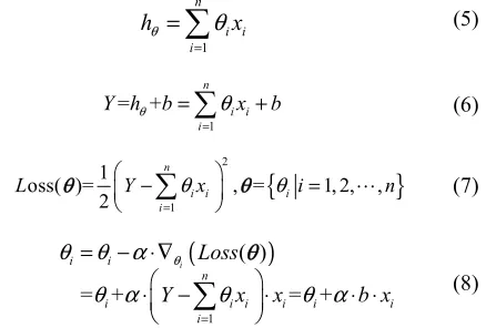
According to the point of view in the paper of Sebastian Ruder [9], given an input data , , and

the coefficients ( ) of existence were assumed that it made the following formula valid (see “(5)”).

If n takes a finite value, there is a bias (b) between the True Value (Y) and the Estimated Value ( ). The formula (see (5)) can be reformed as “(see (6))”. And the loss function can be defined as “(see (7))”. Minimizing the loss value, we can get the formula (see (8)). In the formula above, is the learning rate and b is the bias.

(5)

(6)

(7)

(8)

2.3. Similar Principal Component Analysis (SPCA)

Principal Component Analysis (PCA, see Algorithm 1) algorithm was widely used in dimension reduction, but O'TOOLE [10] deemed that it was unreasonable. HAN [11] gave an improved algorithm called Similar PCA (SPCA) algorithm. The detailed algorithm is shown in Algorithm 2. The dimensions of PCA’s results and SPCA’s results were the same. What's more, SPCA retained some information which discarded by PCA and this can be used for sample generation.

Algorithm 1 PCA

i

n d

x

∈

ℝ× i=1, 2,⋯,n

i θ h_θ

α

1 n i i i

h_θ

θ

x

= =

∑

1 = + n i i i

Y h_θ b θx b

= =

∑

+

{

}

2 1 1

oss( )= , = 1, 2, ,

2

n

i i i

i

L Y θx θ i n

=   − =   

∑

 ⋯ θ θ

(

)

1 ( ) = + = + i i i n

i i i i i i

i

Loss

Y x x b x

Input: { , ,x x_{1 2} ⋯, }=x_n A∈ℝn d× , spatial dimension q.

Output: D={w w1, 2,⋯,wq}.

1: Centralizing of sample data,

1

1 n

i

i i i

x x _n x

=

← −

∑

; 2: Converting the data from the previous step into column vectors, x_i →l_i, X={ , ,l l1 2 ⋯, }ln ;

3: Computing the eigenvalues and eigenvectors of matrices T

XX ;

4: Calculating the eigenvectors corresponding to the largest q eigenvalues w w1, 2,⋯,wq.

Algorithm 2 SPCA Input: A, D, q. Output: D′={ , ,x x1′ ′2 ⋯, }xq′ .

for i=1,⋯,q _do for j=1,⋯,n do

Computing angle

θ

ij between xjand wi,

(0, ) ij

θ ∈ π ;

end for

Sorting θii, and let θ0=argmin(θii), recording the j;

i j

x′ =x .

end for

3. Advanced Cognitive Model (ACM)

3.1. Main Theorem

For the pattern recognition or statistical pattern recognition, Bishop [12] believed that pattern recognition was a combination of theories and methods that contained a great deal of information processing. From the root, there was no accurate definition of this term. Hinton [13, 14] proposed the concept of deep learning and used it to solve the problems in pattern recognition.

For any third-order matrix, defining the formula (3) as true kernel (K), and it can be represented as follows (see “9”).

11 12 13 9

21 22 23 1 31 32 33

= _{i i}

i

a a a

w a a a k K a a a =

 

 

=_{ } ⋅

 

 

∑

(9)

The is the coefficient of (true kernel), the denotes a weight matrix or a convolution kernel. Convolving the weight matrix with the input data matrix (see “(10)”):

x= ⊗w x (10)

And the action mode is “same”. Assuming that a series of results can be linearly combined, which is shown in the formula (6). Lastly, the bias b is the distance between Y and

h_θ, which we named “impression”.

Definition1. Pattern consists of , k_i and . is

expressed as patterns implied by all third-order matrices:

9 9 3 1 1 9 9 1 1 = ( ) (( ) ) i i i i

i j j

i j

P x w x

k K x

θ θ θ = = = = ⋅ = ⋅ ⊗ = ⋅ ⋅ ⊗

∑

∑

∑

∑

(11)

In the formula (11), each w needs to compute one-time summation, and there is just only one impression (b). In order to layering the impression, w was split as follows (see Table 1).

Table 1. Sub w and Corresponding Impressions of P . ₃

Symbol Combination Impression & expression

w 1 b Y P= -₃

1 1=i i

w k ⋅K 9 1

9

1

( ₁ )

b Y _i x

i w θ = − ⊗ = ⋅

∑

36 2 2 1

= ( j j)

j

w k K

= ⋅

∑

36 _{2 1} 36 ₁

1

( ₂ )

i i

b =b − θ w ⊗b

= ′ ⋅

∑

So the Pattern can be rewritten as (see “(12)”):

(12)

The impression b₁ is the bias of 1st layer. The impression

2

b is the bias of 2nd layer. By analogy, the patterns of all fifth-order matrices are as shown in Table 2.

Table 2. Sub w and Corresponding Impressions of P . ₅

Symbol Combination Impression & expression

w 1 b Y P= -5

1 1=i i

w k ⋅K 25 1

25

1

( ₁ )

b Y _i x

i w θ = − ⊗ = ⋅

∑

300 2 2 1

= ( j j)

j

w k K

= ⋅

∑

300 _{2 1} 300 ₁

1

( ₂ )

i i

b =b − θ w ⊗b

= ′ ⋅

∑

The Pattern of P₅ is (see “(13)”):

(13)

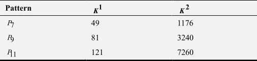
The relative parameters of the expression of P P P7, 9, 11 are shown in Table 3.

Table 3. Sub w and Corresponding Impressions of P P P . ₇, ₉, ₁₁

Pattern K1 K2

7

P 49 1176

9

P 81 3240

11

P 121 7260

i

k K

w

K θi P3

9 36

1 1

1 1

3 31 32

2

( ) ( )

=

+

i i

i w x i w b

P P

P

θ θ = ⊗ = ′⋅ ⊗

+

=

∑

∑

25 300 1 1 1 1

5 51 52

2

( ) ( )

=

+

i i

i w x i w b

P P

P

θ θ

= ⊗ = ′⋅ ⊗

+

3.2. Supplementary Views

In the process of pattern learning, only

θ

is a hyper-parameter to be learned (see“(8)”), and the parameter

k should be artificially designed. Assuming input is single sample image data, the impressions b1 and b2 can be used as data source of pattern discrimination after training. In the process of testing, each test data can be impressed by the pattern learned.

Hypothesis1. If the pattern is learned, for example, if we trained one figure data of number 1, the following statement should hold true:

(1) All numbers mapped to 1 should be recognized as 1 by the pattern;

(2) Numbers other than (1) should not be recognized as 1 by the pattern.

(3) More importantly, the input data can be replaced with other numbers’ data.

Hypothesis2. The training picture data should be more regular, and the impressions after learning can be misidentified.

Methods of data normalization contains normalization of input data [15, 16], normalization of weight data [17]. In this paper, the training data were normalized by 2-norm, each column of training data was divided by the module length of the column. In the process of learning pattern, a drop method was referred to dropout [18] and in order to reduce calculation data (see Algorithm 3), the viewpoint of contribution in the method of PCA [19] was adopted. In the output layer of ACM, function ∆( , )xσ (see “(14)”) is similar with rectified linear unit (ReLU) [20].

Algorithm 3 Drop Input: θ, λ . Output: θ’, ω υ, . 1: Descending order of θ;

2: Calculating the minimum value of mthat satisfies the

formula 1

1 , (0,1) m i i n i i θ λ λ θ = = ≥ ∈

∑

∑

, and let ω=m;

3: θ’ is the larger value of the first ω of θ, and υ is the label of the original position of θ’;

(14)

The pseudo-code of Algorithmic (ACM) computing flow is (see Algorithm 4):

Algorithm 4 ACM

Input: = 1,2, … ,10 , , , K, P, , , and the test data y. (x_i is one of the 0-9 10 graphs.)

Output: Predictive labels l. Learning pattern:

1: Initializing parameter k, , ; Calculating K1 and K2; 2: Bring formula (11) (K1) into formula (7) and updating parameters with formula (8). Using dropout method to get parameter of the 1st layer , ɷ , and the impression b₁;

1

1

1 1 1( )

1

= _{i j} ( _i)

j

b x w x

ω υ θ = ′ −

∑

⋅ ⊗

3: Replacing K1 in step two with K2, and change input data to b₁ in step two, we can get , ɷ , and b₂;

2

2

2 1 2 2( ) 1

1

= _j ( )

j

b b w b

ω υ θ = ′ −

∑

⋅ ⊗ Testing pattern:

4: According to the pattern learned at the 1st layer, 10 types of impressions of training samples are calculated:

1

1

1 1 1( )

1

( )

i i j i

j

b x w x

ω

υ

θ

=

′

= −

∑

⋅ ⊗ , (i=1, 2,⋯,10)

1i= (1i, )

b ∆ b σ

5: Calculating the impression of 1st layer of the test sets:

1

1

1 1 1( )

1

= ( )

y j

j

b y w y

ω

υ

θ

=

′

−

∑

⋅ ⊗ ,b_y1= (∆b_y1, )

σ

6: For the 2nd layer:

2

2

2 1 2 2( ) 1

1

( )

i i j i

j

b b w b

ω

υ

θ

=

′

= −

∑

⋅ ⊗ , (i=1, 2,⋯,10)

2i= ( 2i, )

b ∆b σ ;

2

2

2 1 2 2( ) 1

1

= ( )

y y j y

j

b b w b

ω

υ

θ

=

′

−

∑

⋅ ⊗ , by2= (∆by2, )

σ

1st level prediction: 7: for i =1,…, 10 do

1i ( y1 1i)

d =norm b −b , norm is 2-norm.

1 ( )1

T =min d , the value of i (l₁=i) corresponding to

1

T is the predictive label of y. 2nd level prediction:

8: for i =1,…, 10 do

2i ( y2 2i)

d =norm b −b , norm is 2-norm.

2 ( 2)

T =min d , the value of i (l₂ =i) corresponding to

2

T is the predictive label of y.

4. Experimental Results

4.1. (Q) MNIST Data Set

All experiments were based on the MNIST hand-written digit recognition benchmark. All the images were pre-normalized into a unitary 784-dimensional vector. The data set was divided into a training set with 60000 images ,

= ( , )= 0,

x if x x x

if x

σ

σ  ≥_σ

∆  _<

and a test set with 10000 images.

The QMNIST dataset was generated from the original data found in the NIST Special Database 195 with the goal to match the MNIST preprocessing as closely as possible. The QMNIST test dataset contained the 60000 testing examples.

All the test data were divided into two categories. One was the original test data and the other was that converted the non-zero value of the original test data into 1 (“*”_1, * is the name of test data set). The second category only retained calligraphy. In order to facilitate the calculation with MATLAB, the test set data was collated as shown in the Table 4. MNIST and MNIST_1 test data were matrices with 784 × 10000, QMNIST and QMNIST_1 test data were matrices with 784 × 60000.

The experimental training set was also divided into two categories:

1. From the original training set of 0-9 classes, each class was randomly selected one picture to form a group, lastly, a total of 10 groups and 100 pictures.

2. According to SPCA and Hypothesis2, 0-9 regular library of original library were made based on original library, and saw the regular data as a new training set.

Table 4. The test data set.

MNIST/(MNIST _1) QMNIST/(QMNIST _1) Real

label

Col num Col num

1-980 980 1-5952 5952 0

981-2115 1135 5953-12743 6791 1

2116-3147 1032 12744-18769 6026 2

3148-4157 1010 18770-24853 6084 3

4158-5139 982 24854-30633 5780 4

5140-6031 892 30634-36087 5454 5

6032-6989 958 36088-42044 5957 6

6990-8017 1028 42045-48275 6231 7

8018-8991 974 48276-54165 5890 8

8992-10000 1009 54166-60000 5835 9

Total 10000 60000

Referring to algorithm 4, the experimental flow is shown in Figure 3.

Figure 3. Image of experimental flow.

Random selection of training data

5 https://www.nist.gov/srd/nist-special-database-19.

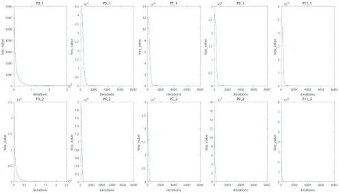
We took a group of data for example (see Figure 4). Using data “0” for training, the original data and normalized data were as follows (see Figure 5). According to algorithm 4, the loss curve under Pattern refer to Figure 6, the impression under Pattern refer to Figure 7. And the correct recognition rate (CRR) on MNIST test set was shown as Table 5. CRR on MNIST test set was shown that all Pattern and two kinds of impressions can map to number 1. However, the recognition rate was very unsatisfactory. CRR on QMNIST test set was shown as Table 6, CRR on QMNIST test set was the similar with MNIST test set, the overall recognition rate was low. There were remaining 99 groups of training results in the first category, referring to the open source link (OSL)6 which included all the recognition results and all the unrecognized results. From the above experimental analysis, the results were closed to Hypothesis1, but not ideal.

Figure 4. Images of training data in MNIST.

Figure 5. Images of training data of “0”.

Regular library of training data

The figure (see Figure 8) was generated based on SPCA. These pictures look much more regular than original handwriting. Similarly, the number 0 was used to train for comparison, the impression under Pattern refer to Figure 9. Experimental data of numbers 1 to 9 were shown in the OSL. The training data of “0” and the normal data were shown as Figure 10. And the training progress was shown in Figure 11 (refer to Algorithm 4), the results (impressions) of intermediate process were shown in Figure 12. The first row (origin_*) is the initial data, the 2nd row is the impression of 1st layer, and the 3rd row is the impression of 2nd layer.

Figure 6. Images of Loss curves corresponding to different modes and layers.

Figure 7. Images of impressions corresponding to different patterns and layers.

Figure 8. Images of regular data.

Figure 10. Images of regular data of “0”.

Figure 11. Data training process.

Figure 12. Figures of impressions corresponding to different modes and layers.

Compared with the 1st category, the CRR on MNIST, MNIST_1, QMNIST, QMNIST_1 test set was shown as Tables 7, 8, 9, 10 respectively. In the end, the learning results

and all the recognition results were shown in the OSL. These results declared that Pattern should be worth exploring and studying.

Table 5. The test results of MNIST.

Pattern CRR Overall rate

0 1 2 3 4 5 6 7 8 9

P3

b1 0.2602 0.6247 0.0814 0.6010 0.1059 0.2377 0.5438 0.5185 0.1756 0.0803 0.3277

Pattern CRR Overall rate

0 1 2 3 4 5 6 7 8 9

P5

b1 0.3102 0.1709 0.1279 0.6327 0.0672 0.3442 0.6409 0.5496 0.3460 0.1031 0.3262

b2 0.3061 0.2123 0.1231 0.6267 0.0733 0.3408 0.5908 0.5263 0.2977 0.1070 0.3182

P7

b1 0.3010 0.1507 0.1240 0.6416 0.0662 0.3330 0.6441 0.5253 0.3860 0.0951 0.3233

b2 0.2867 0.2150 0.1202 0.6426 0.0723 0.3285 0.6127 0.5146 0.3634 0.0942 0.3227

P9

b1 0.3061 0.1304 0.1298 0.6564 0.0601 0.3464 0.6785 0.5545 0.4230 0.0942 0.3340

b2 0.3051 0.1304 0.1289 0.6554 0.0601 0.3475 0.6754 0.5535 0.4220 0.0951 0.3334

P11

b1 0.3071 0.1392 0.1308 0.6307 0.0519 0.3318 0.7296 0.5788 0.4363 0.0951 0.3393

b2 0.3061 0.1383 0.1298 0.6317 0.0519 0.3307 0.7286 0.5788 0.4353 0.0932 0.3386

Trained only one picture (see Figure 5) and let the Pattern on the whole test set (MNIST, 10000). Different patterns and different layers of impressions were used to recognize the 0-9 numbers. The overall recognition rate (ORR) was around 30%.

Table 6. The test results of QMNIST.

Pattern CRR Overall rate

0 1 2 3 4 5 6 7 8 9

P3

b1 0.2772 0.6140 0.0785 0.5411 0.1161 0.2231 0.5488 0.5364 0.1569 0.0865 0.3252

b2 0.2231 0.9246 0.0508 0.4129 0.0666 0.1249 0.3868 0.4282 0.0829 0.0620 0.2886

P5

b1 0.3249 0.1777 0.1279 0.5848 0.0618 0.3421 0.6369 0.5750 0.3095 0.1066 0.3253

b2 0.3149 0.2148 0.1180 0.5771 0.0708 0.3337 0.5855 0.5484 0.2706 0.1093 0.3154

P7

b1 0.3159 0.1635 0.1253 0.5924 0.0649 0.3331 0.6517 0.5595 0.3431 0.0985 0.3251

b2 0.3048 0.2240 0.1162 0.5876 0.0728 0.3277 0.6194 0.5380 0.3156 0.0991 0.3212

P9

b1 0.3184 0.1409 0.1351 0.6050 0.0566 0.3506 0.6792 0.5805 0.3820 0.0982 0.3345

b2 0.3172 0.1408 0.1341 0.6047 0.0566 0.3508 0.6779 0.5794 0.3813 0.0982 0.3340

P11

b1 0.3261 0.1539 0.1391 0.5838 0.0464 0.3326 0.7252 0.5996 0.3961 0.0977 0.3403

b2 0.3253 0.1537 0.1379 0.5845 0.0469 0.3322 0.7239 0.5988 0.3958 0.0973 0.3399

Trained only one picture (see Figure 5) and let the Pattern on the whole test set (QMNIST, 60000). Different patterns and different layers of impressions were used to recognize the 0-9 numbers. The ORR was around 30%.

Table 7. The test results of MNIST.

Pattern CRR Overall rate

0 1 2 3 4 5 6 7 8 9

P3

b1 0.9786 0.6070 0.4273 0.7327 0.2424 0.0078 0.7557 0.3307 0.9138 0.8494 0.5885

b2 0.9745 0.7339 0.4370 0.7545 0.2637 0.0280 0.7599 0.4222 0.9014 0.8741 0.6207

P5

b1 09827 0.7260 0.4709 0.7624 0.2546 0.0101 0.7537 0.4144 0.9055 0.8672 0.6207

b2 0.9796 0.7736 0.4787 0.7683 0.2617 0.0135 0.7516 0.4553 0.8973 0.8751 0.6322

P7

b1 0.9796 0.7260 0.4922 0.7941 0.2851 0.0224 0.7766 0.4718 0.8984 0.8642 0.6370

b2 0.9786 0.7912 0.5000 0.8099 0.2933 0.0404 0.7714 0.5243 0.8778 0.8771 0.6533

P9

b1 0.9857 0.7947 0.5058 0.7851 0.2800 0.0179 0.7474 0.4912 0.8973 0.8672 0.6444

b2 0.9857 0.8035 0.5078 0.7851 0.2811 0.0179 0.7474 0.4990 0.8943 0.8702 0.6465

P11

b1 0.9857 0.7762 0.5281 0.7970 0.3096 0.0247 0.7735 0.5477 0.8922 0.8692 0.6573

b2 0.9857 0.7859 0.5300 0.7990 0.3147 0.0247 0.7693 0.5554 0.8912 0.8692 0.6596

Trained only one picture (see Figure 10) and let the Pattern on the whole test set (MNIST, 10000). Different patterns and different layers of impressions were used to recognize the 0-9 numbers. The ORR was around 60%. Compared with Table 5, ORR had been greatly improved. The recognition rate of digits 0 was higher than that rate of other digits, which illustrated the correctness of hypothesis 1.

Table 8. The test results of MNIST_1.

Pattern CRR Overall rate

0 1 2 3 4 5 6 7 8 9

P3

b1 0.9378 0.9471 0.7471 0.8267 0.7668 0.5348 0.8194 0.8288 0.8285 0.8404 0.8122

b2 0.9378 0.9427 0.7326 0.8168 0.7749 0.5247 0.8278 0.8317 0.8162 0.8157 0.8065

P5

b1 0.9378 0.9524 0.7326 0.8287 0.7688 0.5291 0.8058 0.8307 0.8285 0.8444 0.8105

b2 0.9398 0.9463 0.7306 0.8198 0.7739 0.5291 0.7975 0.8278 0.8234 0.8404 0.8074

P7

b1 0.9398 0.9542 0.7364 0.8376 0.7800 0.5336 0.8173 0.8375 0.8234 0.8424 0.8148

b2 0.9398 0.9498 0.7287 0.8337 0.7862 0.5235 0.8173 0.8405 0.8162 0.8385 0.8120

P9

b1 0.9449 0.9533 0.7364 0.8327 0.7688 0.5404 0.8017 0.8327 0.8214 0.8375 0.8115

b2 0.9449 0.9515 0.7384 0.8317 0.7699 0.5392 0.7996 0.8327 0.8193 0.8375 0.8110

P11

b1 0.9469 0.9542 0.7481 0.8366 0.7709 0.5448 0.8132 0.8375 0.8265 0.8365 0.8160

Trained only one picture (see Figure 10) and let the Pattern on the whole test set (MNIST_1, 10000). Different patterns and different layers of impressions were used to recognize the 0-9 numbers. The ORR was more than 80%. Compared

with Table 7, ORR had been greatly improved. The recognition rate of digits 0 and 1 was higher than that rate of other digits, but other rates were not low, which further verified the correctness of hypothesis1 and hypothesis 2.

Table 9. The test results of QMNIST.

Pattern CRR Overall rate

0 1 2 3 4 5 6 7 8 9

P3

b1 0.9691 0.5977 0.4262 0.6921 0.2545 0.0055 0.7578 0.3130 0.9110 0.8351 0.5802

b2 0.9684 0.7292 0.4403 0.7155 0.2772 0.0246 0.7610 0.4155 0.8905 0.8605 0.6141

P5

b1 0.9713 0.7217 0.4731 0.7204 0.2721 0.0092 0.7546 0.4147 0.8980 0.8622 0.6156

b2 0.9703 0.7721 0.4773 0.7345 0.2779 0.0171 0.7569 0.4628 0.8866 0.8720 0.6294

P7

b1 0.9718 0.7159 0.4890 0.7608 0.3028 0.0227 0.7719 0.4726 0.8878 0.8595 0.6314

b2 0.9713 0.7916 0.4957 0.7788 0.3149 0.0451 0.7737 0.5357 0.8686 0.8751 0.6520

P9

b1 0.9726 0.7975 0.5098 0.7502 0.2979 0.0207 0.7509 0.4945 0.8898 0.8586 0.6414

b2 0.9726 0.8052 0.5113 0.7533 0.2993 0.0224 0.7509 0.5001 0.8869 0.8612 0.6435

P11

b1 0.9758 0.7843 0.5402 0.7643 0.3285 0.0286 0.7740 0.5527 0.8839 0.8641 0.6566

b2 0.9758 0.7959 0.5422 0.7678 0.3310 0.0315 0.7735 0.5612 0.8815 0.8643 0.6596

Trained only one picture (see Figure 10) and let the Pattern on the whole test set (QMNIST, 60000). Different patterns and different layers of impressions were used to recognize the 0-9 numbers. The ORR was around 60%. Compared with Table 7, the ORR was similar.

Table 10. The test results of QMNIST_1.

Pattern CRR Overall rate

0 1 2 3 4 5 6 7 8 9

P3

b1 0.9271 0.9544 0.7484 0.7654 0.7597 0.5372 0.8268 0.8374 0.8024 0.8302 0.8064

b2 0.9232 0.9524 0.7370 0.7827 0.7659 0.5288 0.8286 0.8434 0.7866 0.8070 0.8002

P5

b1 0.9271 0.9560 0.7395 0.7980 0.7661 0.5323 0.8101 0.8437 0.7976 0.8398 0.8056

b2 0.9278 0.9532 0.7376 0.7949 0.7702 0.5275 0.8054 0.8445 0.7905 0.8380 0.8035

P7

b1 0.9289 0.9585 0.7420 0.8044 0.7718 0.5304 0.8289 0.8517 0.7968 0.8386 0.8098

b2 0.9288 0.9566 0.7375 0.8026 0.7798 0.5253 0.8273 0.8556 0.7871 0.8353 0.8082

P9

b1 0.9278 0.9576 0.7426 0.8006 0.7588 0.5455 0.8069 0.8435 0.7930 0.8367 0.8058

b2 0.9278 0.9576 0.7431 0.8013 0.7597 0.5447 0.8064 0.8435 0.7927 0.8367 0.8059

P11

b1 0.9304 0.9589 0.7509 0.8060 0.7637 0.5534 0.8217 0.8514 0.7956 0.8353 0.8112

b2 0.9304 0.9591 0.7506 0.8067 0.7645 0.5539 0.8219 0.8511 0.7944 0.8343 0.8111

Table 11. Average recognition rate for CMU PIE database/%.

WF [22] LTP [23] RM [24] MSR [25] WD [26]

92.59 75.07 78.33 72.20 92.13

GF [27] OGPF [28] AWOGBP [21] ACM

90.07 87.40 95.50 92.00/99.46

Trained only one picture (see Figure 10) and let the Pattern on the whole test set (QMNIST_1, 60000). Different patterns and different layers of impressions were used to recognize the 0-9 numbers. The ORR was more than 80%. Compared with Table 9, ORR had been greatly improved. The recognition rate of digits 0 and 1 was higher than that rate of other digits, but other rates were not low, which further verified the correctness of hypothesis1 and hypothesis 2.

4.2. Experiments on CMU PIE Database

Considering the frontal face samples and the influence of a single factor, for example, lighting changes, CMU PIE [5] and Extended Yale B [6] databases were chosen to conduct experiments. In order to compare with [21], the latest research under the same conditions was selected to design the experiment. In the process of dis-crimination, the average value of each group was subtracted to weaken the influence

of illumination change, and the illumination threshold was set to adjust the optimal value.

Figure 13. Sample images in CMU PIE database.

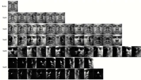
4.3. Experiments on Extended Yale B Database

Considering that the condition of light changes in the CMU PIE database was not complex, ACM was also verified on Extended Yale B database which covered more complex illumination variation in this section. The database included 38 subjects under nine poses and 64 illumination conditions. Most importantly, all the images contained positive face only. The only factor that interfered with positive face recognition was the change in illumination. For comparison, the frontal pose images captured under 64 different lighting conditions for each of the 38 persons. And these images were divided into 5 subsets according to the angle of the light source directions, refer to Table 12.

Table 12. The subset of angles.

Refer Sub1 Sub2 Sub3 Sub4 Sub5

0° 1°-12° 13°-25° 26°-50° 51°-77° others

In our experiments, the images were all resized to 64 × 64. Images with the light condition (0°) were treated as training data, and all the data of subsets were used for testing. The sample images were shown in Figure 14 and Table 13 listed the experiment results on Extended Yale B database.

Table 13. Recognition rate for Extended Yale B/%.

Methods Testing subsets

Sub1 Sub2 Sub3 Sub4 Sub5

WF 99.56 99.34 90.57 85.15 81.16

LTP 98.24 99.12 87.93 82.70 73.26

RM 99.56 99.12 83.77 77.06 71.05

MSR 96.92 97.58 74.12 59.58 45.98

WD 95.17 98.02 82.67 81.57 69.25

GF 99.12 99.12 84.87 70.87 73.27

OGPF 100 99.34 92.33 71.62 66.07

AWOBBP 100 99.34 94.46 90.04 83.93

ACM 1

st _{99.56 99.34 99.12 88.53 93.07}

2nd _{99.56 99.34 98.25 92.48 90.86}

As shown in Table 13, ACM expressed the competitive performance in Sub1, Sub2, and had the best performance in Sub3, Sub4 and Sub5, especially in Sub4 and Sub5 where the illumination conditions are extremely poor. Each layer of ACM deepened the subjective impression of this class. By adjusting the illumination threshold parameters, the influence of illumination changes can be reduced. Hence, we can draw a conclusion that ACM is better for single sample recognition under varying illumination.

Figure 14. Subset images in Extended Yale B database.

5. Conclusion

In the experimental process, we adopted convolution instead of neural network alone, and we got the surprising results under the condition of single sample training. ACM focuses on the shape of the sample itself and learns about it. Regardless of the handwritten number or the face sample, the shape of the sample has not changed, and the learning pattern should be consistent and this has been verified by the experimental results. ACM gives an attempt on pattern recognition. The following parts analyse its characteristics.

5.1. Sparse Property

The K has obvious sparse property. Many algorithms are pursuing sparse property, because the property has the following two advantages: firstly, it has the property of automatic feature selection; lastly, it makes the model easier to interpret. Considering the sparse property, we need to supplement the property in the later stage of the ACM algorithm. For example, increasing the number of layers and making patterns more abundant (refer to Table 14), the sparse property of later patterns will gradually decrease. There are so many combinations that one of the next tasks is studying whether these modes are combined or duplicated or their effects are equivalent.

Table 14. Patterns and Combination Numbers.

Layer P3 P5 P7 P9 P11

L1 9 25 49 81 121

L2 36 300 1176 3240 7260

L3 84 2300 18424 85320

…

L4 126 12650

… …

L5 126 53130

L6 84 177100

L7 36

…

L8 9

L9 1

… …

Last

layer 1 1 1 1 1

5.2. Combining Neural Network Algorithms

bigger sparse property will lead to vanishing gradient, so in the process of debugging parameters of such algorithms, bigger sparse property is generally not allowed. When the sparse property is reduced, the fusion of ACM and DLA is also one of the next tasks.

5.3. Pattern Fusion

In addition to the aforementioned algorithm fusion scheme,

Can we try the pattern fusion?

As the various operators proposed in the traditional algorithms in the past, combining with each other, we can refer to them completely. From the experimental results, the advantages of the patterns itself are not outstanding, such as the results of P3 and P5 are not absolutely superior or inferior. For this reason, another branch of the next task is to study the integration of these models in order to achieve major breakthroughs.

After carefully study of these results, it can be concluded that in the sparse layer, the pattern has learned the common characteristics of samples. The shallow understanding of the algorithm is the common characteristics of the samples. From this point of view, the algorithm should deepen the number of layers, whether it is pattern fusion or algorithm fusion.

In this paper, we proposed ACM algorithm which is a novel pattern recognition model for single sample recognition. Compared with other classical algorithms related to illumination changes, ACM is a more efficient and stable representation in the task of single face sample recognition. ACM combines convolution kernel and drop operation to extract information. And the most important is that the information is extracted from sample which should be expressed regularly, and this has verified by the experiments of (Q) MNIST recognition. ACM is worthy of further study.

Acknowledgements

Xu Han was supported in part by Bureau of Science &Technology Nanchong City Research Grant 18SXHZ0012, Hai-Yun Chen was supported in part by Bureau of Science &Technology Neijiang City Research Grant 2018KJFH003, Shu-Duo Zhao, Chen-Xin Ma and Wen-Hao Zhou were supported in part by Southwest Petroleum University Research Grant NC17SY2003, Jin Xu and Guan-Qin Feng were supported in part by Southwest Petroleum University Research Grant 18SXHZ0011.

References

[1] C. Szegedy, Wei Liu, Yangqing Jia, P. Sermanet, S. Reed, D. Anguelov, D. Erhan, V. Vanhoucke, and A. Rabinovich, “Going deeper with convolutions,” in 2015 IEEE Conference on Computer Vision and Pattern Recognition (CVPR), June 2015, pp. 1–9.

[2] A. K. I. S. R. R. S. Geoffrey E. Hinton, Nitish Srivastava, “Improving neural networks by preventing co-adaptation of

feature detectors,” Computer Science, 2012. arXiv: 1207.0580.

[3] M. D. Zeiler and R. Fergus, “Visualizing and understanding convolutional networks,” Computer Science, 2013. arXiv: 1311.2901.

[4] L. B. Chhavi Yadav, “Cold case: The lost mnist digits,”

Computer Science, 2019. arXiv: 1905.10498.

[5] T. Sim, S. Baker, and M. Bsat, “The cmu pose, illumination, and expression database,” IEEE Transactions on Pattern Analysis & Machine Intelligence, 2003, vol. 25, no. 12, pp. 1615–1618.

[6] A. S. Georghiades, P. N. Belhumeur, and D. J. Kriegman, “From few to many: Illumination cone models for face recognition under variable lighting and pose,” IEEE Transactions on Pattern Analysis & Machine Intelligence, 2002, vol. 23, no. 6, pp. 643–660.

[7] K. Yu, Y. Lin, and J. Lafferty, “Learning image representations from the pixel level via hierarchical sparse coding,” in CVPR 2011, June 2011, pp. 1713–1720.

[8] M. J. Prewitt, “Object enhancement and extraction,” Picture Processing & Psychopictorics, 1970, pp. 75–149.

[9] S. Ruder, “An overview of gradient descent optimization algorithms,” Computer Science, 2016. arXiv: 1609.04747. [10] V. T. B. V. O’Toole A J, Leopold D A, “Prototype-referenced

shape perception: Adaptation and after-effects in a multidimensional face space,” Journal of Vision, 2001. [11] X. J. C. H.-y. HAN Xu, LIU Qiang, “Handwritten numeral

recognition algorithm based on similar principal component analysis,” Computer Science, 2018, vol. 45 (11A), pp. 278– 281, 307.

[12] C. M. Bishop, “Neural networks for pattern recognition,”

Agricultural Engineering International the Cigr Journal of Scientific Research & Development Manuscript Pm, 1995, vol. 12, no. 5, pp. 1235-1242.

[13] G. E. Hinton and R. R. Salakhutdinov, “Reducing the dimensionality of data with neural networks,” Science, 2006, vol. 313, no. 5786, pp. 504–507.

[14] H. G. LeCun Yann, Bengio Yoshua, “Deep learning”, Nature,

2015.

[15] R. A. Parth Sane, “Pixel normalization from numeric data as input to neural networks,” Computer Science, 2017. arXiv: 1705.01809.

[16] A. D. Samit Bhanja, “Impact of data normalization on deep neural network for time series forecasting,” Computer Science, 2018. arXiv: 1812.05519.

[17] M. S. Maximilian Schmidt, “Normalizing flows for novelty detection in industrial time series data,” Computer Science, 2019. arXiv: 1906.06904.

[18] N. Srivastava, G. Hinton, A. Krizhevsky, I. Sutskever, and R. Salakhutdinov, “Dropout: A simple way to prevent neural networks from overfitting,” Journal of Machine Learning Research, 2014, vol. 15, no. 1, pp. 1929–1958.

[20] R. H. Hahnloser, Sarpeshkar, R., M. A. Mahowald, R. J. Douglas, and H. S. Seung, “Digital selection and analogue amplification coexist in a cortex-inspired silicon circuit,”

Nature, 2000, vol. 405, no. 6789, pp. 947–951.

[21] H. X. Yang and Y. Y. Cai, “Adaptively weighted orthogonal gradient binary pattern for single sample face recognition under varying illumination,” Iet Biometrics, 2016, vol. 5, no. 2, pp. 76–82.

[22] B. Wang, W. Li, W. Yang, and Q. Liao, “Illumination normalization based on weber’s law with application to face recognition,” IEEE Signal Processing Letters, 2011, vol. 18, no. 8, pp. 462–465.

[23] T. Xiaoyang and T. Bill, “Enhanced local texture feature sets for face recognition under difficult lighting conditions,” Amfg, 2007, vol. 4778, no. 6, pp. 1635–1650.

[24] N. S. Vu and A. Caplier, “Illumination-robust face recognition using retina modeling,” in IEEE International Conference on Image Processing, 2010.

[25] D. J. Jobson, Rahman, Z., and G. A. Woodell, “A multiscale retinex for bridging the gap between color images and the human observation of scenes,” IEEE Transactions on Image Processing, 2002, vol. 6, no. 7, pp. 965–976.

[26] T. Zhang, B. Fang, Y. Yuan, Y. T. Yuan, Z. Shang, D. Li, and F. Lang, “Multiscale facial structure representation for face recognition under varying illumination,” Pattern Recognition, 2009, vol. 42, no. 2, pp. 251–258.

[27] Z. Taiping, T. Yuan Yan, F. Bin, S. Zhaowei, and L. Xiaoyu, “Face recognition under varying illumination using gradientfaces,” IEEE Transactions on Image Processing, 2009, vol. 18, no. 11, pp. 2599–2606.